2. THE STATISTICAL MODEL AND MOTIVATION

Consider a model for the relationship between a dependent variable

and a set of explanatory variables

, such that the conditional distribution of Y given X and T belongs to the following family of density functions indexed by θ and η₁,…,η_p:

where Θ is assumed to be a compact subset of

are, respectively, compact subsets in

are also assumed to be compact sets

.

The relationship between Y and (X,T) will be fully characterized by determining the values of θ and η₁, η₂,…,η_p, where θ is an unknown parameter vector and η_j's are assumed to be unknown smooth functions of not necessarily disjoint subsets of

, that take values in a set

More precisely, η₁ = η₁(x¹), η₂ = η₂(x²),…,η_p = η_p(x^p), where the vectors

, may contain common elements.

For the sake of simplicity, we will consider X and T absolutely continuous random variables defined in a compact support. This is by no means necessary; we could also include discrete or even dummy variables, especially for T, replacing the densities by probabilities measures. For the variable X that will enter into the nonparametric estimation part we refer to Delgado and Mora (1995). They show that the impact of discrete variables can be handled nonparametrically in the same way and does not even affect the rate of convergence.

Note that our approach is fairly general and nests all separable models. In fact, the structure of the model will depend on the family of conditional densities into which it will be assumed to fall. That is, the functional form of [ell ](·|T;η₁,η₂,…,η_p;θ) will be determined not only by the statistical assumptions but also by the restrictions introduced by economic theory.

To explain our considerations further we present one example from economics where separability and/or limited dependency is of essential interest. Gronau (1973) proposes a theory of how a housewife decides whether or not to work and how much to work. He assumes that the wage offered, W^o, is given to each housewife independently of the hours worked H. Then, given a W^o, a housewife maximizes her utility function U(C,X¹,X²) subject to X = W^oH + V and C + H = Time, where C is time spent at home for child care, X = (X¹,X²) represents all other goods, Time is total available time, and V is other income. Thus, a housewife does not work if

and does work if the inequality is reversed. If she works, the hours of work H and the actual wage rate W must be such that

Gronau calls the left-hand side of the preceding equation the housewife's value of time, i.e., the reservation wage, W^r. If the utility function U(·) is strongly separable in the bundles of goods X¹ and X², then Gronau's model could be statistically described as follows:

where he assumes that the pair (u_1i,u_2i) are independent and identically distributed (i.i.d.) random variables generated from a bivariate Gaussian distribution with zero mean, variances σ₁², σ₂², and covariance σ₁₂.

Note that in this example we have considerably weakened Gronau's assumptions because we are allowing for η₁(·) and η₂(·) to be unknown smooth functions of the different variables instead of imposing, as he did, that w^o and w^r be writable as linear combinations of the independent variables. As already remarked in many studies, linearity is often imposed for the sake of simplicity in the specification of the statistical model but without justification from economic theory. Unfortunately, if our interest lies in weakening the restrictions that concern the index function, we cannot at the same time relax the assumptions about the conditional distribution of the error term. Therefore, for the sake of identification, we need to take the conditional density of the error term as known.

In model (2) we are interested in estimating the parameters θ = (σ₁²,σ₂²,σ₁₂) and the unknown functions η₁(·) and η₂(·). Just to simplify further discussion we impose for the sake of simplicity σ₁₂ = 0. This condition is used in Gronau (1973); however, as already remarked in Amemiya (1985), this is a rather unrealistic assumption, and in fact it is not necessary for estimation purposes. Then, the full likelihood based on the statistical model that is described in (2) is

where F is the cumulative standard normal distribution and f is its density,

is the product over all observations without jobs, and

is the product overall with jobs. Note that (3) represents a multiple-index model where the nonparametric components are introduced into the structural model additively.

The assumption of strong separability of the utility function can be relaxed, e.g., by introducing weak separability between the bundles X¹ and X². Then Gronau's model can take the following alternative form:

and the full likelihood expression for model (4) takes the form

In this case (5) represents a multiple-index model where the nonparametric components are introduced in a nonadditive manner. Certainly, a further possibility for relaxing the model would be to make use of latent separability, i.e., allowing for some regressors to appear in both X¹ and X².

Following this example, it is also possible to develop a structural model where the participation (binary choice) equation in (2) and (4) is replaced by a truncated Tobit model. This extension is based on Heckman's model (Heckman, 1974), which differs from Gronau's model in that the determination of hours worked, H, is included in the model. If we are only interested in the hours of work (H) we have the following truncated Tobit model:

where X and T are characterized at the beginning of Section 2. Assume also that the error term, u, is normally distributed with zero mean and variance σ². Then it could be interesting to model h(·) in various ways: a partially linear model, a semiparametric partially additive model (strong separability), or weaker forms of separability such as weak or latent separability. Under the preceding assumptions the truncated Tobit model has the following likelihood function:

Setting θ = (γ^T,σ)^T we again face one of the regression problems discussed. Compare also Section 4.

In the preceding examples, we have given reasons for working with a wide class of semiparametric structural econometric models that present estimation problems that are far from trivial and, to our knowledge, remain unsolved: the estimation of censored and truncated models under different types of separability restrictions. Certainly, in the much simpler case of a single regressor on [0,1] , Conditions I, S, and NP of Severini and Wong (1992) allow censored or truncated variables. Under the assumption of strong separability, alias additive models, a wide class of estimators has been already reviewed in Section 1. However, the assumption of separability is much weaker than additivity. It allows for any combination and interaction between the component functions, as can be realized in (4). The main advantage of the estimation procedure proposed in this paper is that it can handle a wide class of separable models jointly with any kind of nonparametric multi-index structure, as we have in (2) or (4).

3. THE ESTIMATOR

Suppose we have a sample of N independent replicates {(Y_i,X_i,T_i)}_i=1,…,N. Our goal will be to estimate jointly the parameter vector θ ∈ Θ and the nuisance parameters η₁, η₂,…,η_p. If as stated in Section 1 the conditional density of Y given X and T belongs to the family of parametric functions represented in (1) we could write the following likelihood function:

and then maximize it over the parameters of interest. Estimation of a finite-dimensional parameter in the presence of an infinite-dimensional nuisance parameter has been considered by a number of authors. Here, we propose estimators that are based on a generalized profile likelihood approach (see Severini and Wong, 1992). The estimation procedure consists of approximating the likelihood function locally through a weighted likelihood approach developed in Staniswalis (1989). Furthermore, under certain hypotheses on the likelihood function we also develop an estimator that is based on maximizing a local quasi-likelihood function (see McCullagh and Nelder, 1989; Severini and Staniswalis, 1994). The main advantage of the method based on the quasi-likelihood function is that there is no need to assume knowledge of the conditional density function. However, its drawback is that it rules out the possibility of considering the multiple-index models that are typical in standard microeconomic analysis.

Let us denote the estimators of the different curves at point x₀ by

. The estimation is then implemented through a three-step procedure. The steps are as follows.

and set

for all j = 1,2,…,p.

The first two steps are derived from the generalized profile likelihood approach proposed in Severini and Wong (1992) but extended to the case in which θ, η₁,…,η_p, and X are multidimensional. From these two steps we obtain a root-N-consistent, efficient estimator of θ₀, but unfortunately the nonparametric components are estimated with the problem of the curse of dimensionality.

The third step is included to reduce the curse of dimensionality (d is reduced to d_j) of the nonparametric estimators. Furthermore, it is also argued that this third step is oracle efficient, i.e., as efficient as the infeasible estimate that is based on knowing all components but the one of interest. This property has been discussed in the context of additive models (see Linton, 1997, 2000) and is extended here to weak and latent separable models.

Let us introduce some notation and assumptions that will be used in the remainder of the paper. Denote by p(X) the marginal density of X = (X¹,…,X^p) and by p_j(X^j) the marginal density of X^j. Further, set σ²(x) = E [Y²|X = x] , σ_j²(x^j) = E [Y²|X^j = x^j] , and

Here, F_j(·) can be, respectively,

. Let μ_x denote a k-vector of nonnegative integer constants. For such a vector we define

(i)

, where μ_x = (μ₁,…,μ_k)^T,

(ii) for any function a(x) on

:

Now, we require that the family of density functions

satisfy the following conditions:

(A.1). For fixed but arbitrary θ₁,η₁⁺,…,η_p⁺, where θ₁ ∈ Θ, and η₁⁺ ∈ H₁,…,η_p⁺ ∈ H_p, let

If θ ≠ θ₁, then

Let I_θ(η₁,η₂,…,η_p,θ) denote the marginal Fisher information for θ in the parametric model, i.e.,

where

and

Then assume that the matrix I_θ(η₁,η₂,…,η_p,θ) is positive definite for all θ ∈ Θ and η₁ ∈ H₁,…,η_p ∈ H_p.

(A.2). Assume that for vectors |r_η| ≤ 4 and |s_θ| ≤ 4 such that |r_η| + |s_θ| ≤ 4 the function

exists for almost all Y and T. Further, assume that

Condition (A.1) is an identification condition. It is equivalent to Condition I of Severini and Wong (1992, p. 1777). Condition (A.2) is standard in likelihood-related problems, and it allows differentiation and integration to be interchanged when differentiating

This assumption is equivalent to Condition S of Severini and Wong (1992, p. 1777).

Next, we need to include some smoothness assumptions that are necessary because of the use of nonparametric smoothing methods.

(B.1). For each θ ∈ Θ and

let us define

Then

for 2 ≤ |r_η| ≤ 4, |s_θ| ≤ 2, |t_x| ≤ 1, and |r_η| + |s_θ| + |t_x| ≤ 4.

(B.2). Let the vector η_θ(x) = (η_1,θ(x¹),…,η_p,θ(x^p))^T be the solution to

with respect to η for each fixed θ and x. Here η_θ(x) is unique, and for any constant ε > 0 there exists another δ > 0 such that

implies that

for j = 1,…,p.

(B.3). We define

and let f_θ^(r_η,s_θ) (y,t|x) denote the conditional density of Δ_η,θ^r_η,s_θ (Y,T) given X = x. Then

These smoothness assumptions affect the rate of convergence of the nonparametric estimators of the different components η₁,…,η_p. In fact, in the Appendix it is shown that (B.1)–(B.3) are sufficient conditions to prove that the nonparametric estimators

, from Step I, have the following properties:

Property (i) provides the slowest rate of convergence that the nonparametric estimators must fulfill to allow

(in step 2) to achieve the

rate. The estimators proposed by Klein and Spady (1993) and Ichimura and Lee (1991), e.g., satisfy this property. Property (ii) imposes an asymptotic orthogonality condition between the parametric and the nonparametric estimators. This implies that the asymptotic distribution of

is not affected by the distribution of

and therefore the parametric estimator achieves the marginal Fisher information for θ. Properties (i) and (ii) are equivalent to what is called Condition NP in Severini and Wong (1992, p. 1779).

Finally, we also need to impose some conditions on K(·) and h_N. The main conditions are as follows.

(K.1). The kernel K(·) is a real valued function on

such that it is compactly supported with

,

and

(H.1). h_N is a sequence of constants satisfying h_N = O_P(N^−α),

such that m/d > (q − p − 2)/(2p + q + 4).

To have mean square error converging to zero, if d ≥ 4, Assumption (H.1) implies bandwidth rates of order α < ¼. Thus m must be larger than 2. By Assumption (K.1) this implies a higher order kernel. This is a standard bias reducing technique, and jointly with Assumption (H.1) on the bandwidth it is needed to achieve the preceding condition of N^1/4-consistency. Note finally that the bandwidth rates required in condition (H.1) are faster than the optimal ones. This is also standard in semiparametric models and is due to the fact that the bias of the nonparametric estimator would otherwise appear in the asymptotic properties of the parametric part.

Then, if

is the solution to optimization problem (9) in step 2, the following result is proved in the Appendix.

THEOREM 1. Under Assumptions (A.1), (A.2), (B.1)–(B.3), (K.1), and (H.1), as N tends to infinity

and

As can be observed from this result, the semiparametric estimator achieves the semiparametric efficiency bound (see Chamberlain, 1992; Newey, 1990, 1994). Note that our model restrictions do not contain any information about a possible dependence structure between X and T. Further note that the asymptotic variance could be approximated with the aid of the Hessian matrix.

Following the example introduced in Section 2, in Gronau's model with strong separability (see equation (2)), the nonparametric estimators for η₁ and η₂ are obtained by maximizing the smoothed log-likelihood version of (3) and then

The finite-dimensional parameter σ₁² can be estimated by maximizing the unsmoothed log-likelihood version of (3),

whereas

is a solution of an implicit formula expression.

Then, under the conditions stated in Theorem 1, we obtain the following result:

and

If instead of using strong separability, alias additivity, in Gronau's model, we use weak separability as in equation (4), then the estimator in step 1 for η₁ is the same as in the additive case, but for η₂ we obtain the expression

for

. Further expressions can be obtained as in the strongly separable case.

Next we study the asymptotic behavior of the nonparametric estimators obtained in step 3. To do this, we introduce the following additional assumptions.

(C.1). Nh_j^d_j → ∞ and Nh_j^d_j+4 → 0, for j = 1,…,p, as N tends to infinity.

(C.2). The support of kernel K_j is compact and ∫tK_j(t) dt = 0, for any j.

(C.3). For all j = 1,…,p it holds that

Assumptions (C.1)–(C.3) are standard in nonparametric regression literature. For example, condition (C.1) makes variance and bias tend to zero when the sample size increases. The condition Nh_j^d_j+4 → 0 can be weakened by assuming only that h_j → 0. Then, under the previous assumptions we obtain

Therefore, the asymptotic distribution of

will have a nonnegligible bias of order O(Nh_j^d_j+4). To correct the bias, two alternative procedures are available in the relevant literature. One is to approximate the distribution of

, e.g., by a bootstrap or subsampling technique (see Section 5). The other approach is to assume that the bandwidth h_j tends to zero slightly faster than the optimal rate, i.e., Nh_j^d_j+4 → 0. We have chosen the second procedure, although we remark that at this rate of decay of the bandwidth, our nonparametric estimator will achieve a rate of convergence that is slightly slower than the optimal rate. Condition (C.3) is an identification condition that is similar in additive models under Gaussian errors to the backfitting algorithm (see Hastie and Tibshirani, 1990). Under these assumptions the following theorem holds.

THEOREM 2. Under the conditions of Theorem 1 and Assumptions (C.1)–(C.3), for any j = 1,…,p

Remark. Note that under correct specification of the statistical model the information equality holds, H_j(η_j,θ₀) = I_j(η_j,θ₀), and then the asymptotic variance in (18) collapses to

As an example, in Gronau's model with strong separability (see equation (2)) under the conditions assumed in Theorem 2, the estimator for η₁(x₀¹) obtained in step 3 has the closed form

and shows the following asymptotic behavior:

as N tends to infinity, where

In the weakly separable case of equation (4), in step 3 we obtain the same estimator for η₁ as in the additive case. However, its asymptotic variance is different. In this case, it can be shown that

As can be noticed from the theorem, all nonparametric components are estimated at the fastest possible rate overcoming the curse of dimensionality. This agrees with the results found by Stone (1986) for additive models, but we remark that the same result is achieved here with a weaker restriction on separability. Also, as indicated before, we reach the same asymptotics as if the other components in the model were known. Finally, the (pointwise) asymptotic expressions could be estimated without too much extra calculation. Unfortunately, it is well known that in finite samples these estimates of asymptotic expressions are of little practical help. Instead, we again refer to Section 5.

In some contexts, the results obtained in Theorems 1 and 2, mainly consistency and Gaussian limiting distribution, still hold even if only part of the model is correctly specified. More precisely, by taking a one-parameter linear exponential family as the conditional distribution of Y given X, maximum likelihood estimates of the parameters of interest are consistent and asymptotically normal. The quasi-likelihood approach allows us to estimate models up to the identifiable (separable) components whenever they present a single-index structure.

Each member of the family has a density that can be written as

where δ = (η₁,…,η_p,θ). In this case, by the properties of the exponential density function, one gets

where g(·) is a known function. Note that again heteroskedasticity is included but the variance function V₀ must depend on T and X through the index g(t,η₁(x¹),…,η_p(x^p),θ₀). In this case, it is possible in steps 1–3 to replace the log-likelihood log

by the quasi-likelihood function r(·,g(t,η₁(x¹),…, η_p(x^p),θ₀)) defined as

where V(·) is a known function. If we replace the true distribution by the quasi-likelihood function in all steps of our estimation procedure, then, as shown in Rodríguez-Póo, Sperlich, and Vieu (2000), the preceding results still hold. However, as might be expected, there is an efficiency loss if the specification is not equivalent to the real distribution.

To show the main results of this section we need to make the following assumptions.

(Q.2). For p = 1,…,3 then ∂^pV(g)/∂g^p exists and is bounded for all

.

(Q.3). The function g(·) is at least three times continuously differentiable bounded with respect to all its arguments.

(B.1′). As for (B.1) replacing φ(·) by r(·).

(B.2′). As for (B.2) replacing φ(·) by r(·).

(B.3′). As for (B.3) replacing φ(·) by r(·).

(C.3′). For all j = 1,…,p

Assumptions (Q.1)–(Q.3) are regularity conditions needed in the quasi-likelihood framework mainly to guarantee that the quasi-likelihood function used in estimating η₁,…,η_p and θ has the properties of a likelihood function. Condition (C.3′) is the same as the identification condition (C.3) but now in terms of the quasi-likelihood function.

THEOREM 3. Under Assumptions (B.1′)–(B.3′), (K.1), (H.1), and (Q.1)–(Q.3), as N tends to infinity

As can be seen now, if the model is correctly specified both criterion functions coincide, and therefore we obtain the efficient estimator that was shown in Theorem 1.

The behavior of the estimator obtained in step 3 is given in the following theorem.

THEOREM 4. Under the conditions of Theorem 3 and Assumptions (C.1), (C.2), and (C.3′), we have for any j = 1,…,p

where

as N tends to infinity.

From Theorem 4 we remark on two important issues: the estimator is oracle efficient, i.e., as efficient as the infeasible estimate that is based on knowing all components except the one of interest. Moreover, this estimator avoids the curse of dimensionality. Linton (2000) proposes a two-step estimator for the additive components in a generalized additive (i.e., strongly separable) nonparametric regression model. In our approach, if we adopt a generalized additive model, the asymptotic variance given in Theorem 4 collapses to the variance given in Linton (2000, Theorem 1, p. 506). This result was expected because, for the strongly separable case, to obtain the estimators for the additive components Linton proposes a local linear approximation, whereas we propose a local constant one. As is well known (see Fan, 1992), the difference between the two types of approximation is in the bias, but the variance stays the same. Both estimators avoid the curse of dimensionality, but Linton's does not consider the weak and latent separability case.

4. COMPUTATIONAL ASPECTS AND SIMULATIONS

In this section we deal with some questions that are relevant in practice and illustrate the numerical performance of our estimators by some simulations. After a bandwidth discussion we come back to the model examples from Section 2, beginning with the censored Tobit model. Second, we consider a truncated Tobit and weak separability. In that example we also discuss the problem when the nonparametric part of the model of interest cannot be completely identified in step 1. For those cases we suggest a feasible, well performing algorithm, for which we also present a small simulation study.

Unfortunately, the choice of bandwidth or the corresponding smoothing parameters in spline-, wavelet-, etc., smoothing is still an open problem in multidimensional regression and testing. From a mathematical point of view there exists an optimal bandwidth in the sense that the mean squared error is minimized. Even though for our estimators plug-in methods and cross validation are both possible in theory the inexactness of the asymptotic expressions in finite samples and computational burdens renders these approaches impractical. On the other hand, one has to admit that in our context of estimating flexible functional forms non- and semiparametric methods are explorative tools, maybe even just for finding the proper parametric model. Looking at matters in that way, an increase in the bandwidth simply corresponds to a decrease in the degrees of freedom, unfortunately allowing an increasing bias toward constant functionals. An extension of our approach to a local linear smoother would relax this to a bias toward linear functionals (cf., e.g., Lejeune, 1985). But this is left open for future research. Note that these considerations do not hold for the problem of testing parametric vs. nonparametric functionals. There, the optimal bandwidth is the one that guarantees the correct significance level, which is usually a different bandwidth from the mean squared error minimizing one. As a consequence of all this, the empirical researcher should apply various bandwidths, always depending on their “tolerance” against smoothness or wiggliness. This holds especially for the choice of the h_j's in step 3.

In step 1, bandwidth h_N has to be chosen appropriately to yield good estimates for the parametric part of the model. This can be handled by considering the nonparametric part as nuisance parameters. Then, as can also be seen from theory (e.g., in condition (H.1)), one should undersmooth in step 1. All we need there for the nonparametric part is sufficient smoothness to reach convergence in the maximization algorithm. Therefore, in practice we choose bandwidths close to the smallest ones that still yield numerical convergence in steps 1 and 2. In applications on real data some additional weighting or trimming could be useful for points at the boundary or outliers.

How can a possibly unwanted double effect of h_N on step 3 be avoided? We speak of double effect because the final estimates

are affected not only by the estimate of θ but also by the preestimates of the η_j, j = 1,…,p. As indicated in Section 3, the asymptotic results in Theorems 2 and 4 do not change if we use consistent preestimates different from those proposed. So one could, e.g., repeat step 3 without changing the theoretical results. This means in practice that by only one iteration in step 3, one can limit the impact of h_N (on the final estimates of the η_j) to the impact caused by

. This allows us to consider the bandwidth choices in steps 1 and 3 separately.

4.1. Example 1—Censored Tobit

As mentioned previously, we come back to the censored Tobit models introduced in Section 2. We first consider the strong separable one; i.e., we generate data from

with η₁(x) = η₂(x) = 2.0 + 2.0/(exp{−10x} + 1) and u_i,v_i being independently drawn from N{0,1} and observing

.

Here, we have chosen the same functional form for η₁ and η₂ to compare them afterward. One might expect that the information lacking (by not observing w^r) would worsen the estimation of η₂ and σ_v compared to η₁, σ_u. We implement a procedure that maximizes the likelihood:

as did Gronau (1973), where F is the cumulative standard normal distribution and f its density.

As we know that correlation between the covariates worsens the estimation results for estimators such as marginal integration and backfitting (see Sperlich, Linton, and Härdle, 1999) sometimes by a great deal, we draw N = 500 observations (x¹,x²)^T from N{0,Σ} with variances of 1.0 and covariances σ₁₂ = 0.3. Further, for the simulation it is more convenient to have all data inside a given interval; therefore we transform each variable by x → 0.55(2.4 arctan(x)/π + 1.0) − 0.55, thus projecting all observations into the interval [−0.55, 0.55] . Then the functions η₁, η₂ are estimated on a grid of 30 points from −0.5 to 0.5.

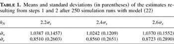
In step 1 we try bandwidths h_N = 2.2σ_x, 2.4σ_x, 2.6σ_x, where σ_x indicates the vector of the standard deviations of x₁, x₂. Here, σ_x is close to the smallest bandwidth without running into numerical problems. Condition (H.1) requires higher order kernels in step 1. As q in (H.1) can be quite large, a kernel of order m = 4 is sufficient, and we choose the “optimal” fourth-order kernel (see Lejeune, 1985). Mean and standard deviation of

after performing 250 simulation runs for each bandwidth h_N are displayed in Table 1.

Means and standard deviations (in parentheses) of the estimates resulting from steps 1 and 2 after 250 simulation runs with model (22)

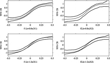
In step 3 higher order kernels are no longer, necessary and we choose the quartic one, which is of order 2. As bandwidths we try h := (h₁,h₂)^T = 0.8σ_x, (h₁,h₂)^T = 1.0σ_x, and 1.2σ_x. Note that this leads to nine different estimates (three different h_N times three different h) for η₁, η₂ from which in Figure 1 are given some selected results when using h_N = 2.4σ_x in step 1. The results are displayed in terms of 95% pointwise confidence bands (without bias correction) calculated from 250 simulation runs. The dashed lines are the data generating functions.

95% pointwise confidence bands of (left), (right) from model (22) for bandwidths hT = 0.8σx in the upper row, and hT = 1.2σx in the lower one. The construction of the confidence band (c.b.) is based on 250 replications with hN = 2.4σx. Dashed lines represent the data generating functions.

First, as expected we discover clearly the bias and boundary effects, especially when choosing a large h in step 3. Further, one can see how the underestimation of σ_v leads to confidence bands for η₂ much wider than for η₁. Finally, as a result of the “information loss” of not observing w^r but w^o, η₂ is clearly estimated with less exactness than η₁. Nevertheless, despite the complexity of the model and highly correlated regressors the real shapes can be detected by our procedure quite well.

We now consider an example extending the estimation problem in three directions: weak separability, higher dimensions, and nonidentifiability in step 1.

4.2. Example 2—Truncated Tobit

Let us turn to a problem we so far have not explicitly discussed. Consider a truncated Tobit model as introduced in Section 2:

with

, and

Recalling the likelihood function, the problem we face here is that in steps 1 and 2 we cannot uniquely identify η₁,η₂,…,η₄ but only γ, σ_u, and η. The estimation algorithm we suggest in that case is as follows: first proceed to steps 1 and 2 for γ, σ_u, and η. Then in step 3 solve a simultaneous equation system for the smoothed likelihoods of

up to

making use of the estimates obtained in steps 1 and 2.

A computationally feasible way is an iteration in step 3 over the four likelihoods for the

as we have already suggested in the context of bandwidth discussion. The major difference here is that as a result of the identification problem in step 1, we do not have all necessary consistent preestimates at hand as demanded in Theorems 2 and 4. Although it is known that the derivation of a closed asymptotic theory for such an algorithm is impossible, it is a most intuitive procedure, known from operations research to converge under some regularity (smoothness) conditions and providing the right thing, i.e., the estimates presented in our theorems. The preestimates lacking in step 3 would be replaced by appropriately flexible parametric estimates. In our simulation study we use simply linear preestimation for η₁ to η₃ and start the iteration over η₄. Obvious extensions of our method that would allow identification but also the derivation of asymptotic theory are discussed in the next section.

The data generating process is model (23) with η₁(x) = 1.0, η₂(x) = 2x² − 1, η₃(x) = sin(2x), η₄(x) = x, γ = (−1.5,2.0)^T, and σ_u = 1.0. The regressors are drawn independently with t₁,t₂ ∼ U [0,2] and x_j ∼ U [−1,1] for j = 1,…,4. We draw about 700 observations to end up always with N = 600 nontruncated (y > 0.0) observations. For the estimation we apply the identification condition E [η₂] = E [η₃] = E [η₄] = 0 even though this is quite restrictive for η₄. However, simulations without fixing the expectation of η₄ lead to identification problems for η₃ and η₄.

Again we have to choose a higher order kernel in step 1 (compare condition (H.1)). Note that because of the identification problem p is just equal to 1 in steps 1 and 2. With q large, a kernel of order m = 6 is sufficient to fulfill (H.1). We choose the “optimal” sixth-order kernel (see Lejeune, 1985) but the quartic one in step 3. Our bandwidths are h_N = 4.0σ_x and h = (0.6,0.6,0.6,0.9)^Tσ_x, respectively.

After 500 replications we get for

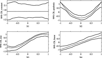
in the mean (−1.5051, 2.0115, 1.1105) with standard deviations (0.09733, 0.10479, 0.059). Figure 2 gives the 99% pointwise confidence bands for the estimators of η₁ to η₄, again without bias correction and based on 500 replications. The dashed lines are the data generating functions.

99% pointwise confidence bands for all function estimates from the upper left to the lower right, based on 500 replications. Dashed lines are the data generating functions.

In Figure 2 we detect slight boundary effects, and certainly the bands for the functional η₁, i.e., the constant, are quite wide because we estimate it without fixing the mean E [η₁] . But otherwise the estimation procedure works quite well and always detects the correct functional form even in this high-dimensional, complex model with only N = 600 observations.