2. Shock model theory

Suppose that a system is subjected to a sequence of shocks which arrive randomly in time according to a counting process $ \lbrace N(t)\colon t\geq 0 \rbrace$ and cause damage to the system. Assume that the system under consideration is not subject to constant wear and tear and only the shocks are responsible for its failure. Let $\bar{P}_k$ be the probability that the system survives the first k shocks, $k=0, 1, 2, \ldots,$ and suppose T denotes the time to failure. We assume that the $\bar{P}_k$ satisfy the following natural condition:

\begin{equation*} 1= \bar{P}_0 \geq \bar{P}_1 \geq \bar{P}_2 \geq \cdots .\end{equation*}

The probability of the system surviving beyond time t is given by the survival function

(1) \begin{equation} \bar{H}(t)\,{:}\,{\raise-1.5pt{=}}\, \mathbb{P}(T>t)=\sum_{k=0}^{\infty} \mathbb{P} (N(t)=k )\bar{P}_k.\end{equation}

At this juncture it is pertinent to mention that shock model theory plays a vital role in diverse areas (see Nakagawa [Reference Nakagawa44], Finkelstein and Cha [Reference Finkelstein and Cha21] and the references therein). Before proceeding further, a motivating example would be appropriate. Consider an insurance company where claims arrive randomly in time. Claims can be interpreted as ‘shocks’ and the magnitude $X_i$ of the ith claim can be interpreted as the damage caused by the ith shock. When the total claim exceeds a threshold Y (insurance company’s capital), the company goes bankrupt. This idea is applicable in various scenarios such as risk analysis, inventory control, dam theory, biometry, etc., by simply considering appropriate analogues. For instance, ‘shock’, ‘system failure’ and ‘survival until time t’ can be substituted, respectively, by ‘claim’, ‘bankruptcy’ and ‘all claims met during [0, t]’ in risk analysis or by ‘demand’, ‘shortage’ and ‘no shortage during [0, t]’ in inventory control; for more details, see A-Hameed and Proschan [Reference A-Hameed and Proschan2]. Using the prior knowledge of the fact that the survival function $\bar{H}(t)$ belongs to a certain class of life distributions, it is feasible to obtain sharp bounds on the survival function and other parameters of the distribution. Such knowledge produces proper maintenance strategies in reliability contexts, higher accuracy in estimation results and functional financial policies in risk analysis. In the huge body of literature concerning shock model theory, the works of Shanthikumar and Sumita [Reference Shanthikumar and Sumita49], Anderson [Reference Anderson4], Yamada [Reference Yamada52], Kochar [Reference Kochar37], Pérez-Ocón and Gámiz-Pérez [Reference Pérez-Ocón and Gámiz-Pérez47], Pellerey [Reference Pellerey46], Ebrahimi [Reference Ebrahimi17] and others are significant.

An underlying fundamental question which is inextricably linked to reliability shock models is as follows: If the sequence $ \lbrace\bar{P}_k \rbrace_{k=0}^{\infty}$ possesses a certain discrete ageing property (such as IFR, IFRA, NBU, NBUE and so on), does $\bar{H}(t)$ inherit the corresponding continuous version of the said ageing property under the transformation (1) when N(t) is a homogeneous Poisson process (HPP), non-homogeneous Poisson process (NHPP), stationary or non-stationary pure-birth process.

For the IFR, IFRA, NBU, NBUE and decreasing mean residual life (DMRL) classes, Esary et al. [Reference Esary, Marshall and Proschan18] provided an affirmative answer to the above question when N(t) is an HPP. A-Hameed and Proschan [Reference A-Hameed and Proschan1] showed that under some assumptions on the intensity function $\Lambda(t)$, the same preservation result holds for the above classes when N(t) is an NHPP. Later they also considered the same problem for the above classes when shocks arrive according to stationary and non-stationary pure-birth processes and proved analogous results; see A-Hameed and Proschan [Reference A-Hameed and Proschan2]. Stronger results in a similar vein are available for the NBUE, harmonic new better than used in expectation (HNBUE) and $\mathcal{L}$ classes in Block and Savits [Reference Block and Savits15], Klefsjö [Reference Klefsjö31] and Klefsjö [Reference Klefsjö33] respectively. Thereafter, analogous results for the new better than used in failure rate (NBUFR) and new better than average failure rate (NBAFR) classes of life distributions were derived by Abouammoh et al. [Reference Abouammoh, Hindi and Ahmed3] and Fagiuoli and Pellerey [Reference Fagiuoli and Pellerey19]. Shock models leading to bivariate IFR and DMRL distributions are discussed in Ghosh and Ebrahimi [Reference Ghosh and Ebrahimi22]. In the context of non-monotonic ageing phenomena, Mitra and Basu [Reference Mitra and Basu43] were the first to establish such results for the NWBUE and BFR classes. Anis [Reference Anis5] established the analogous result in the context of IDMRL distributions. We now proceed to establish the corresponding results in the context of classes of life distributions based on the MTTF function. We first recall the notions of discrete versions of DMTTF and IMTTF properties introduced by Li and Xu [Reference Li and Xu39].

In the same spirit, we now introduce the notions of discrete versions of IDMTTF and DIMTTF properties.

Definition 4. A distribution ${P}_k=1-\bar{P}_k$, $k\in \mathbb{N}$, is said to be D-IDMTTF$(k_0)$ (D-DIMTTF$(k_0)$) if there exists $ k_0 \geq 1$ such that

\begin{equation*} \dfrac{1}{P_k}\sum_{i=0}^{k-1}\bar{P}_i = \begin{cases} \text{is increasing (decreasing) in \textit{k} for $ k<k_0$,}\\[4pt] \text{is decreasing (increasing) in \textit{k} for $k\geq k_0$,} \end{cases}\end{equation*}

where D-IDMTTF (D-DIMTTF) denotes discrete IDMTTF (DIMTTF).

We are now in a position to develop shock model theory for pure-birth processes.

2.1. Pure-birth shock models

Now consider a pure-birth shock model where a system is subjected to shocks governed by a birth process with intensities ${\lambda _k}$, $k=0,1,2,\ldots.$ Let $V_{k+1}$ denote the interarrival time between the kth and $(k+1)$th shocks. Assume the $V_{k}$ are independent with $V_{k+1}$ being exponentially distributed with mean ${1}/{\lambda _k}$ for $k=0,1,2,\ldots.$ Then the survival function $ \bar{H}(t)$ of the system can be written as

(2) \begin{equation} \bar{H}(t)=\sum_{k=0}^{\infty} Z_k(t)\bar{P}_k\end{equation}

with

\begin{equation*}Z_k(t)\,{:}\,{\raise-1.5pt{=}}\, \mathbb{P} (N(t)=k ),\end{equation*}

where N(t) is the pure-birth process defined above. We assume that the intensities $ \lbrace \lambda _k \rbrace _{k=0}^{\infty}$ are such that the probability of infinitely many shocks in (0, t] is 0 (i.e. $\sum_{k=0}^{\infty} Z_k(t)=1$), which is equivalent to the condition $\sum_{k=0}^{\infty} \lambda _k^{-1}=\infty$; see Feller [20, page 452]. To develop sufficient conditions for the preservation of DMTTF (IMTTF) properties, we will use the following lemmas.

Lemma 1. (A-Hameed and Proschan [Reference A-Hameed and Proschan2].) Let $Z_k(t)$ be as defined in (2). Then

\begin{equation*}\int_0^t Z_k(u)\,{\textrm{d}} u = \dfrac{1}{\lambda _k}\sum_{j=k+1}^{\infty}Z_j(t).\end{equation*}

Lemma 2. If for any $c\in \mathbb{R}$, $\int_0^t \bar{H}(u)\,{\textrm{d}} u -c H(t)$ has at most one change of sign from $+$ to $-$, then H(t) is DMTTF.

Proof. Suppose $0<x_1<x_2$. We want to show that $M_{H}(x_1)\geq M_{H}(x_2)$. Note that for any $c\in \mathbb{R}$, $\int_0^t \bar{H}(u)\,{\textrm{d}} u -c H(t)$ has at most one change of sign from $+$ to $-$. So this happens for $c_1$ and $c_2$ in particular. By choice of $c_i$, $i=1,2$, we have

\begin{equation*} \int_0^t \bar{H}(u)\,{\textrm{d}} u \begin{cases} \geq c_i H(t) & \text{for $ t\leq x_i$,}\\[3pt] \leq c_i H(t) & \text{for $ t > x_i$.} \end{cases}\end{equation*}

If possible, let $c_1=M_{H}(x_1)< M_{H}(x_2)=c_2$. Take $x_1<t<x_2$. Then

\begin{equation*}\int_0^t \bar{H}(u)\,{\textrm{d}} u \leq c_1 H(t) < c_2 H(t) \leq \int_0^t \bar{H}(u)\,{\textrm{d}} u,\end{equation*}

a contradiction. Thus $M_{H}(x_1)\geq M_{H}(x_2)$ and hence H(t) is DMTTF.

In the next theorem we show how the D-DMTTF (D-IMTTF) property is inherited by the survival function $\bar{H}(t)$ defined in (1).

Theorem 1. Suppose that $\bar{H}(t)$ is defined as in (2). Then H(t) is DMTTF (IMTTF) if

\begin{equation*}\dfrac{1}{P_j}\sum_{k=0}^{j-1}\dfrac{\bar{P}_k}{\lambda _k}\end{equation*}

is decreasing (increasing) in j, where $j\in\mathbb{N}$.

Proof. Note that

\begin{equation*} \bar{H}(t)=\sum_{k=0}^{\infty}Z_k(t)\bar{P}_k \quad \text{and}\quad H(t)=\sum_{k=0}^{\infty}Z_k(t)P_k=\sum_{k=1}^{\infty}Z_k(t)P_k\quad \text{as $P_0=0$.} \end{equation*}

Now for any $c\in \mathbb{R}$ we have

\begin{align*} \int_0^t \bar{H}(u)\,{\textrm{d}} u -c H(t) & = \int_0^t \sum_{k=0}^{\infty}Z_k(u)\bar{P}_k \,{\textrm{d}} u - c \sum_{k=0}^{\infty}Z_k(t)P_k \\ & = \sum_{k=0}^{\infty} \bar{P}_k \int_0^t Z_k(u)\,{\textrm{d}} u - c \sum_{k=0}^{\infty}Z_k(t)P_k \\ & = \sum_{k=0}^{\infty} \bar{P}_k \dfrac{1}{\lambda_k}\sum_{j=k+1}^{\infty}Z_j(t)- c \sum_{k=0}^{\infty}Z_k(t)P_k \quad (\text{by Lemma} {hameedlemma}{1}) \\& = \sum_{j=1}^{\infty} Z_j(t) \sum_{k=0}^{j-1}\dfrac{\bar{P}_k}{\lambda_k} - c \sum_{j=1}^{\infty}Z_j(t)P_j \\& = \sum_{j=1}^{\infty} Z_j(t) \Biggl[ \sum_{k=0}^{j-1}\dfrac{\bar{P}_k}{\lambda_k} - c P_j \Biggr] .\end{align*}

By hypothesis,

\begin{equation*}\sum_{k=0}^{j-1}\dfrac{\bar{P}_k}{\lambda _k} - c P_j\end{equation*}

has at most one change of sign, and if one change of sign occurs, it is from $+$ to $-$. Hence, by the variation diminishing property, it follows that the same conclusion can be drawn for $\int_0^t \bar{H}(u)\,{\textrm{d}} u -c H(t)$. Now an application of Lemma 2 yields that H(t) is DMTTF. The proof for the dual class is analogous.

A pure-birth process reduces to an HPP if all the $\lambda _k$ are equal to $\lambda$. Then Theorem 16 of Li and Xu [Reference Li and Xu39] is obtained as an easy corollary of Theorem 1.

Corollary 1. When N(t) is an HPP, the survival function $\bar{H}(t)$ possesses the DMTTF (IMTTF) property if the sequence $ \lbrace P_k \rbrace_{k=0}^{\infty}$ belongs to the D-DMTTF (D-IMTTF) class.

Now we consider the non-stationary pure-birth shock model of A-Hameed and Proschan [Reference A-Hameed and Proschan2]: shocks occur according to a Markov process; given that k shocks have arrived in (0, t], the probability of a shock occurring in $ (t, t + \Delta t ]$ is $\lambda _k \lambda(t)\Delta t + {\textrm{o}}(\Delta t)$, while the probability of more than one shock occurring in $ (t, t + \Delta t ]$ is ${\textrm{o}}(\Delta t)$. The probability of one shock arriving in a time interval of length $\Delta t$ is allowed to depend on the time point t and also on the number k of shocks that have already arrived, and this dependence is conveyed via the function $\lambda(t)$ and a sequence of constants $\lambda _k$ respectively. Here ${\textrm{o}}(h)$ stands for any function f satisfying

\begin{equation*}\lim_{h\rightarrow 0} \dfrac{f(h)}{h}=0.\end{equation*}

Using Remark 1.1 of A-Hameed and Proschan [Reference A-Hameed and Proschan2], the survival function $ \bar{H}^*(t)$ of the system for this shock model can be written as

(3) \begin{equation} \bar{H}^*(t)=\sum_{k=0}^{\infty} Z_k(\Lambda(t))\bar{P}_k, \end{equation}

where $Z_k(t)$ is as defined in (2) and $\Lambda(t)=\int_0^t \lambda(u) \,{\textrm{d}} u $. Before proving the preservation result in this more general set-up, we first establish the following theorem.

Theorem 2. Let F be DMTTF (IMTTF) and $g\colon [0,\infty)\rightarrow[0,\infty)$ be a differentiable convex (concave) function such that $g(0)=0$. Then $R(t)=F(g(t))$ is DMTTF (IMTTF).

Proof. Assume that F is DMTTF with density f. Now

\begin{align*} \dfrac{{\textrm{d}}}{{\textrm{d}} t} \biggl[ \dfrac{\int_0^t \bar{R}(u) \,{\textrm{d}} u}{R(t)}\biggr] & \stackrel{\textrm{sgn}} = R(t)\bar{R}(t)- \dfrac{{\textrm{d}} R}{{\textrm{d}} t}\int_0^t \bar{R}(u) \,{\textrm{d}} u \\& \stackrel{\phantom{\textrm{sgn}}}{=} F(g(t)) \skew3\bar{F}(g(t)) - f(g(t))g^{\prime}(t) \int_0^t \skew3\bar{F}(g(u)) \,{\textrm{d}} u \\& \stackrel{\phantom{\textrm{sgn}}}{\leq} F(g(t)) \skew3\bar{F}(g(t)) - f(g(t)) \int_0^t \skew3\bar{F}(g(u))g^{\prime}(u) \,{\textrm{d}} u\end{align*}

since $g^{\prime}(x),$ the derivative of g(x) with respect to x, is increasing. Putting $y=g(u)$ in the integral, we get

\begin{equation*} F(g(t)) \skew3\bar{F}(g(t))-f(g(t))\int_0^{g(t)} \skew3\bar{F}(y) \,{\textrm{d}} y \leq 0,\end{equation*}

since F is DMTTF. Hence R is DMTTF. We can draw the same conclusion using limiting arguments even if F does not have a density. An analogous result can be obtained for the IMTTF class of distributions by simply reversing the inequalities.

We are now in a position to prove the following theorem.

Theorem 3. Suppose $\lambda(t)$ is an increasing (decreasing) function and

\begin{equation*} \dfrac{1}{P_j}\sum_{k=0}^{j-1}\dfrac{\bar{P}_k}{\lambda _k} \end{equation*}

is decreasing (increasing) in j, where $j\in\mathbb{N}$. Then $\bar{H}^*(t)$ is DMTTF (IMTTF).

Proof. Note that

\begin{equation*} \bar{H}^*(t)=\bar{H}(\Lambda(t))=\sum_{k=0}^{\infty} Z_k(\Lambda(t))\bar{P}_k . \end{equation*}

One can easily show that $\Lambda (t)=\int_0^t \lambda(u) \,{\textrm{d}} u $ is a convex function since $\lambda(u)$ is increasing. Now applying Theorem 2, it is enough to show that H(t) is DMTTF, which follows from Theorem 1. Similarly, we can establish the same preservation results for the dual class.

A non-stationary pure-birth process reduces to an NHPP if all the $\lambda _k$ are equal to $\lambda$. Equation (3) now yields, as a special case, the following corollary, which is just Theorem 17 of Li and Xu [Reference Li and Xu39].

Corollary 2. When N(t) is an NHPP, the survival function $\bar{H}(t)$ possesses the DMTTF (IMTTF) property if the sequence $ \lbrace P_k \rbrace_{k=0}^{\infty}$ belongs to the D-DMTTF (D-IMTTF) class.

Now we will investigate the same preservation for the non-monotonic classes IDMTTF and DIMTTF in the case of Poisson flow of shocks, i.e. N(t) is a homogeneous Poisson process with intensity $\lambda>0$. Before proving the main result, we will, for completeness, state a result which is proved in Belzunce et al. [Reference Belzunce, Ortega and Ruiz11] using total positivity theory.

Lemma 3. (Belzunce et al. [Reference Belzunce, Ortega and Ruiz11].) Suppose that $ \lbrace {\alpha_k}/{\beta_k} \rbrace_{k=0}^{\infty}$ is a real sequence with the property that

\begin{equation*} \dfrac{\alpha_k}{\beta_k} \begin{cases} \textit{is increasing (decreasing) in \textit{k} for $ k<k_0$,}\\[3pt] \textit{is decreasing (increasing) in \textit{k} for $ k\geq k_0$,} \end{cases}\end{equation*}

for some positive integer $k_0$ and also assume that the power series defined by

\begin{equation*}\Phi(s)\,{:}\,{\raise-1.5pt{=}}\, \sum_{k=0}^{\infty}\dfrac{\alpha_k}{k!}s^k,\quad s\geq 0\quad\text{and}\quad\psi(s)\,{:}\,{\raise-1.5pt{=}}\, \sum_{k=0}^{\infty}\dfrac{\beta_k}{k!}s^k,\quad s \geq 0\end{equation*}

converge absolutely for all $s\geq 0$. Then there exists $s_0\in\mathbb{R}$ such that

\begin{equation*} \dfrac{\phi(s)}{\psi(s)} \begin{cases} \textit{is increasing (decreasing) in \textit{s} for $ s<s_0$,}\\[3pt] \textit{is decreasing (increasing) in \textit{s} for $ s\geq s_0$.} \end{cases}\end{equation*}

Theorem 4. Let $ \lbrace\bar{P}_k \rbrace_{k=0}^{\infty}$ be a sequence of D-IDMTTF $(i_0)$ (D-DIMTTF $(i_0))$. Then $\bar{H}(t)$ is IDMTTF (DIMTTF) if N(t) is an HPP.

Proof. For a homogeneous Poisson shock model,

\begin{equation*} \bar{H}(t)=\sum_{k=0}^{\infty} \,{\textrm{e}}^{-\lambda t}\dfrac{(\lambda t)^k}{k !}\bar{P}_k. \end{equation*}

Now

\begin{align*} \int_0^t \bar{H}(u) \,{\textrm{d}} u & = \int_0^t \sum_{k=0}^{\infty} \,{\textrm{e}}^{-\lambda u}\dfrac{(\lambda u)^k}{k !}\bar{P}_k \,{\textrm{d}} u \\[3pt] & = \sum_{k=0}^{\infty} \dfrac{\bar{P}_k}{\lambda} \int_0^t \dfrac{\lambda^{k+1}}{\Gamma(k+1)}\,{\textrm{e}}^{-\lambda u} u^k \,{\textrm{d}} u \\[3pt] & = \sum_{k=0}^{\infty} \sum_{i=k+1}^{\infty} \dfrac{\bar{P}_k}{\lambda} \dfrac{(\lambda t)^i}{i!}\,{\textrm{e}}^{-\lambda t} \\[3pt] & = \dfrac{ {\textrm{e}}^{-\lambda t}}{\lambda} \sum_{i=1}^{\infty} \dfrac{(\lambda t)^i}{i!} \Biggl( \sum_{k=0}^{i-1}\bar{P}_k\Biggr) ,\end{align*}

and

\begin{equation*}M_H(t) = \dfrac{\displaystyle\frac{ {\textrm{e}}^{-\lambda t}}{\lambda} \sum_{i=1}^{\infty} \frac{(\lambda t)^i}{i!} \Biggl( \sum_{k=0}^{i-1}\bar{P}_k\Biggr)}{\displaystyle\sum_{k=0}^{\infty} \,{\textrm{e}}^{-\lambda t}\frac{(\lambda t)^k}{k !}{P}_k}= \dfrac{1}{\lambda} \dfrac{\displaystyle\sum_{k=1}^{\infty}\frac{(\lambda t)^k}{k!}\sum_{j=0}^{k-1}\bar{P}_j}{\displaystyle\sum_{k=1}^{\infty} \frac{(\lambda t)^k}{k!} P_k} \notag.\end{equation*}

We want to show that the function $M_H(t)$ is increasing in $(0, t_0)$ and decreasing in $[t_0, \infty)$ for some $t_0\geq 0$. Putting $s=\lambda t$, since $\lambda >0$ and $t\geq 0$ it is enough to show that for some $s_0\geq 0$

(4) \begin{equation}\dfrac{\displaystyle\sum_{k=1}^{\infty}\frac{s^k}{k!}\Biggl(\sum_{j=0}^{k-1} \bar{P}_j \Biggr)}{\displaystyle\sum_{k=1}^{\infty} \frac{s^k}{k!}P_k}\begin{cases}\text{is increasing in \textit{s} for $ s<s_0$,}\\ \text{is decreasing in \textit{s} for $ s\geq s_0$.}\end{cases}\end{equation}

Writing $i-1$ in place of k in Lemma 3, if

\begin{equation*}\biggl\lbrace \dfrac{\alpha_{i-1}}{\beta_{i-1}}, i=1,2,\ldots \biggr\rbrace\end{equation*}

is increasing in i for $i<i_0$ and decreasing in i for $i\geq i_0$, then there exists some $s_0\geq 0$ such that

(5) \begin{equation}\dfrac{\displaystyle\sum_{i-1=0}^{\infty}\frac{s^{i-1}}{(i-1)!}\alpha_{i-1}}{\displaystyle\sum_{i-1=0}^{\infty}\frac{s^{i-1}}{(i-1)!}\beta_{i-1}}\begin{cases}\text{is increasing in \textit{s} for $ s<s_0$,}\\ \text{is decreasing in \textit{s} for $ s\geq s_0$.}\end{cases}\end{equation}

Now the expression before the parenthesis in (4) can be written as

\begin{equation*}\dfrac{\displaystyle\sum_{i=1}^{\infty}\frac{s^{i-1}}{(i-1)!}\Biggl(\frac{1}{i}\sum_{j=0}^{i-1} \bar{P}_j \Biggr)}{\displaystyle\sum_{i=1}^{\infty} \frac{s^{i-1}}{(i-1)!}\biggl(\frac{P_i}{i}\biggr)}= \dfrac{\displaystyle\sum_{i-1=0}^{\infty}\frac{s^{i-1}}{(i-1)!}\alpha_{i-1}}{\displaystyle\sum_{i-1=0}^{\infty}\frac{s^{i-1}}{(i-1)!}\beta_{i-1}},\end{equation*}

which is the same as the expression before the parenthesis in (5), where

\begin{equation*}\alpha_{i-1}=\dfrac{1}{i}\sum_{j=0}^{i-1}\bar{P_j}\end{equation*}

and $\beta_{i-1}=P_i/i$. Note that

\begin{equation*}\dfrac{\alpha_{i-1}}{\beta_{i-1}}=\dfrac{1}{P_i}\sum_{j=0}^{i-1}\bar{P}_j\begin{cases}\text{is increasing in \textit{i} for $ i<i_0$,}\\ \text{is decreasing in \textit{i} for $ i\geq i_0$,}\end{cases}\end{equation*}

by the D-IDMTTF property which implies $\bar{H}(t)$ is IDMTTF. The proof for the dual class is analogous.

2.2. The cumulative damage shock model

In this model, each arriving shock causes damage of random magnitude to the system. The system fails when the accumulated damage exceeds a certain threshold. If there is significant individual variation in the ability to withstand shocks, this threshold must, of necessity, be regarded as a random variable Y having a CDF G with $G(0)=0$. Let $X_i$ be the damage caused to the system by the ith shock, $i=1, 2, 3, \ldots .$ We assume that $X_1, X_2, X_3, \ldots $ are independent with CDFs $F_1, F_2, F_3, \ldots $ and are further independent of the critical threshold. Here the $F_i$ and G are lifetime distributions as damage and critical threshold, respectively, are positive. Now the probability of surviving k shocks is

\begin{equation*}\bar{P}_k =\mathbb{P} [X_1+X_2+\cdots + X_k \leq Y ],\quad k=1, 2, \ldots .\end{equation*}

Clearly $\bar{P}_0=1$ and for $k=1, 2, \ldots,$

(6) \begin{equation}\bar{P}_k=\int_0^{\infty} F^{[k]}(x) \,{\textrm{d}} G(x), \end{equation}

where $F^{[k]}$ is used to denote the convolution defined by $F_1*F_2*\cdots*F_k.$ Esary et al. [Reference Esary, Marshall and Proschan18] established that the survival probabilities preserve the discrete NBU property for all choices of life distributions ${ \lbrace F_j \rbrace}_{j=1}^{\infty}$ having $F_j (x)$ decreasing in j for all x if and only if G is NBU. Later A-Hameed and Proschan [Reference A-Hameed and Proschan2] and Klefsjö [Reference Klefsjö31] considered a more special choice of the distributions $ \lbrace F_j \rbrace_{j=1}^{\infty}$ where for all $j=1, 2, \ldots,$

(7) \begin{equation} F_j(x)=\int_0^{x} \dfrac{b^{a_j}t^{a_j-1}}{\Gamma(a_j)}\,{\textrm{e}}^{-b t} \,{\textrm{d}} t, \quad x\geq 0, \ a_j,b>0 . \end{equation}

Then (6) can be explicitly written as

(8) \begin{equation} \bar{P}_k=b \int_0^{\infty} \bar{G}(x) \,{\textrm{e}}^{-b x} \dfrac{(b x)^{A_k-1}}{\Gamma(A_k)} \,{\textrm{d}} x , \end{equation}

where $A_k=\sum_{j=1}^k a_j$. At this juncture we now prove the appropriate theorem in the context of DMTTF and IMTTF distributions.

Theorem 5. Let the survival probability $\bar{P}_k$ be as defined in (8) for $k=1, 2, \ldots$ and $\bar{P}_0=1$, where the damage distributions $F_k$ are given by (7). If $A_k=k+1$ and $\bar{G}$ is DMTTF (IMTTF) then $\bar{P}_k$ is DMTTF (IMTTF).

Proof. Now

\begin{align*} \sum_{j=0}^{k-1} \bar{P}_j & = b \sum_{j=0}^{k-1} \int_0^{\infty} \bar{G}(x) \,{\textrm{e}}^{-b x} \dfrac{(b x)^{j}}{j!} \,{\textrm{d}} x \\[2pt] & = b \int_0^{\infty} \bar{G}(x) \sum_{j=0}^{k-1}\,{\textrm{e}}^{-b x} \dfrac{(b x)^{j}}{j!} \,{\textrm{d}} x \\[2pt] & = b \int_0^{\infty} \bar{G}(x) \biggl( b \int_x^{\infty} \,{\textrm{e}}^{-b y } \dfrac{(b y)^{k-1}}{(k-1)!} \,{\textrm{d}} y \biggr) \,{\textrm{d}} x \\[2pt] & = b \int_0^{\infty} \biggl( \int_0^x \bar{G}(y) \,{\textrm{d}} y \biggr) \,{\textrm{e}}^{-b x } \dfrac{(b x)^{k-1}}{(k-1)!} \,{\textrm{d}}(b x).\end{align*}

Thus, for $c\in \mathbb{R}$,

\begin{equation*}\sum_{j=0}^{k-1} \bar{P}_j - c P_k = b \int_0^{\infty} \biggl[ \int_0^x \bar{G}(y) \,{\textrm{d}} y - \dfrac{c}{b} G(x) \biggr] \,{\textrm{e}}^{-b x } \dfrac{(b x)^{k-1}}{(k-1)!} \,{\textrm{d}}(b x).\end{equation*}

Note that $\int_0^x \bar{G}(y) \,{\textrm{d}} y - ({{c}/{b}}) G(x)$ has at most one change of sign in $x\geq 0$, and if one change of sign occurs, it is from $+$ to $-$. Again we know that the kernel $ {\textrm{e}}^{-b x } {{(b x)^{k-1}}/{(k-1)!}}$ is $\text{TP}_{\infty}$ in $x\geq 0$. Now using the variation diminishing property of totally positive functions, the same conclusion can be argued for $\sum_{j=0}^k \bar{P}_j - c P_k$. This implies that ${{P_k}^{-1}}\sum_{j=0}^{k-1}\bar{P}_j$ is decreasing in k. Hence $\bar{P}_k$ is DMTTF. The proof in the context of the dual class is similar.

3. Weak convergence of IDMTTF distributions

Suppose $\mathcal{C}$ denotes a specific class of life distributions. Let $F_n,\,\, n=1,2, \ldots$ be a sequence of life distributions belonging to $\mathcal{C}$ and $F_n \rightarrow F$ in law. If $F\in\mathcal{C}$, we say that $\mathcal{C}$ is closed under the formation of weak limits. This has been established in the context of monotonic ageing classes such as IFR (Basu and Simons [Reference Basu and Simons10]), HNBUE (Basu and Bhattacharjee [Reference Basu and Bhattacharjee9]) etc. Similarly, in the case of non-monotonic ageing classes, weak convergence of the NWBUE, BFR and IDMRL families have been studied (see Mitra and Basu [Reference Mitra and Basu41,Reference Mitra and Basu42] and Anis [Reference Anis5]). We investigate the above question for the IDMTTF class. Suppose

\begin{equation*}x^*(F)= \inf \lbrace t>0 \colon F(t)>0 \rbrace \geq 0 \end{equation*}

denotes the lower end point of the support of a distribution $F\in L^1$ on $[0, \infty)$. We start by proving an important theorem which will be used to prove the main theorem of this section.

Proof. Choose any $x>x^*(F)$. Then there exists $n_0(x)$ such that $n\geq n_0(x)$ implies $F_n(x)>0$. Now the corresponding MTTF function given by

\begin{equation*}M_{F_n}(x)=\dfrac{1}{F_n(x)}\int_0^x \skew3\bar{F}_n(u) \,{\textrm{d}} u , \quad n\geq n_0(x)\end{equation*}

exists and is finite for every such x, since $F_n(x)$ is positive and $\skew3\bar{F}_n(u)I_{(0,\, x)}(u)$ is bounded by an integrable function g(u) which is given by

\begin{equation*}g(u)=\begin{cases}1 & \text{when $ u \in(0, x)$,} \\0 & \text{otherwise},\end{cases}\end{equation*}

where I denotes an indicator function. Now, by Lebesgue’s dominated convergence theorem, we get

\begin{equation*}\lim_{n\rightarrow\infty} \int_0^x \skew3\bar{F}_n(u) \,{\textrm{d}} u =\int_0^x \skew3\bar{F}(u) \,{\textrm{d}} u , \end{equation*}

so that

\begin{equation*}M_{F_n}(x)=\dfrac{1}{F_n(x)}\int_0^x \skew3\bar{F}_n(u) \,{\textrm{d}} u \rightarrow \dfrac{1}{F(x)}\int_0^x \skew3\bar{F}(u) \,{\textrm{d}} u = M_{F}(x) \quad \text{as}\ n\rightarrow \infty .\end{equation*}

So $M_{F_n}(x)$ converges to $M_F(x)$ at every point $x>x^*(F)$ as $n\rightarrow\infty$.

Next we apply this theorem to prove closure under weak convergence for IDMTTF distributions.

Proof. For an IDMTTF distribution G, we define

\begin{equation*}T_G= \lbrace t_0\colon M_G(t) \,\, \text{is increasing in}\,\,(0,t_0) \,\, \text{and decreasing in} \,\, [t_0, \infty) \rbrace .\end{equation*}

Let $t_{0n} \in T_{F_n}$, $n=1,2, \ldots$ and consider the following two cases.

Case I: $ \lbrace t_{0n} \rbrace_{n=1}^{\infty}$ is bounded. Since $ \lbrace t_{0n} \rbrace$ is bounded, applying the Bolzano–Weierstrass theorem we get a subsequence $ \lbrace t_{0n_k} \rbrace$ of $ \lbrace t_{0n} \rbrace$ converging to some finite limit $\alpha$ as $k\rightarrow \infty$. So for a given $\epsilon>0$ there exists $k_0\geq 1$ such that

\begin{equation*}\alpha - \epsilon < t_{0n_k} <\alpha + \epsilon \quad \text{for all } k\geq k_0 .\end{equation*}

Choose any $x, y > 0$ such that $x<y<\alpha -\epsilon$. Since $M_{F_{n_k}}(t)$ is increasing in $t \in (0, t_{0n_k})$, we have $M_{F_{n_k}}(x) \leq M_{F_{n_k}}(y)$. Taking limits of both sides as $k \rightarrow \infty$ and using Theorem 6, we get $M_F(x) \leq M_F(y)$. Hence $M_F(t)$ is increasing in $(0, \alpha - \epsilon)$. An analogous argument shows that $M_F(t)$ is decreasing in $(\alpha + \epsilon, \infty)$. Consequently, $\alpha\in T_F$, since $\epsilon>0$ is arbitrary. Thus F is IDMTTF with $\alpha$ as one of its change points.

Case II: $ \lbrace t_{0n} \rbrace_{n=1}^{\infty}$ is unbounded. Since $ \lbrace t_{0n} \rbrace$ is unbounded, there exists a subsequence $ \lbrace t_{0n_k} \rbrace$ such that $t_{0n_k}\rightarrow \infty$ as $k\rightarrow \infty$. Choose any $x, y >0$ such that $x<y<\infty$. Then there exists $k_0\geq 1$, sufficiently large, such that

\begin{equation*} x \leq y < t_{0n_k} \quad \text{for all } k\geq k_0 .\end{equation*}

Now $M_{F_{n_k}}(t)$ is increasing in $t \in (0, t_{0n_k})$ implies $M_{F_{n_k}}(x) \leq M_{F_{n_k}}(y)$. Thus $M_F(x) \leq M_F(y)$ on taking limits as $k \rightarrow \infty$ and using Theorem 6 once again. Hence $M_F(t)$ is IMTTF, i.e. IDMTTF with change point at infinity.

As a by-product of the proof of Theorem 7, we get the following theorem.

Proof. If $ \lbrace t_{0n} \rbrace$ is bounded above then the proof follows trivially as in Case I of the proof of Theorem 7 as $\alpha = t_0$, since F has a unique change point. From Case II in the proof of Theorem 7, we get that if $ \lbrace t_{0n} \rbrace$ is unbounded then F is necessarily an IMTTF distribution and hence it has a unique change point at infinity. Now suppose that $ \lbrace t_{0n} \rbrace$ does not converge to infinity. Then there exists $B>0$ such that $t_{0n}\leq B$ infinitely often, so that one can choose a subsequence $ \lbrace t_{0n_k} \rbrace$ converging to a finite limit $\beta$, say. But Case I in the proof of Theorem 7 and uniqueness of the change point of F shows that $\infty=\beta <\infty$, a contradiction. So in this case $t_{0n} \rightarrow \infty$ as $n\rightarrow \infty$, thus establishing our claim.

Theorem 9. Suppose $F_n,\, n=1, 2, \ldots $ is a sequence of IDMTTF life distributions with mean $\mu_n$ and change point $t_{0n}$. Suppose that both the sequences $ \lbrace\mu_n \rbrace_{n=1}^{\infty}$ and $ \lbrace t_{0n} \rbrace_{n=1}^{\infty}$ are bounded and $F_n\rightarrow F$ in law where F is a continuous distribution function. Then, for every $r>0$,

\begin{equation*} \lim_{n\rightarrow\infty}\int_0^{\infty} x^r \,{\textrm{d}} F_n(x)= \int_0^{\infty} x^r \,{\textrm{d}} F(x) .\end{equation*}

Proof. From Theorem 5 of Izadi et al. [Reference Izadi, Sharafi and Khaledi26], we get that for all $n=1, 2, \ldots,$ $F_n$ is NWBUE with change point $\tau_{0n}$ (in the NWBUE sense), say, and $\tau_{0n}< t_{0n}$ since $F_n$ is IDMTTF with change point $t_{0n}$ (in the IDMTTF sense). By Theorem 7, F is IDMTTF and hence F is NWBUE. Now, applying Theorem 4.1 of Mitra and Basu [Reference Mitra and Basu41], we get the desired result.

Proof. Direct application of Theorem 5 of Izadi et al. [Reference Izadi, Sharafi and Khaledi26] shows that F is also NWBUE with change point $x_0$ (in the NWBUE sense), say, and $x_0<t_0$. Hence using Corollary 3.5 (iv) of Mitra and Basu [Reference Mitra and Basu41], we get that for all $ r\geq 1$,

\begin{equation*} \mathbb{E}_F(X^r)\,{:}\,{\raise-1.5pt{=}}\, \int_0^{\infty} x^r \,{\textrm{d}} F(x)\leq \mu^r \Gamma (r+1) \,{\textrm{e}}^{(x_0/\mu)} ,\end{equation*}

from which it follows that the power series $\sum_{r=0}^{\infty} ({{u^r}/{r!}}) \mathbb{E}_F(X^r)$ has a non-null radius of convergence. The theorem now follows from a result of Loève [Reference Loève40, page 217].

Theorem 9 implies that under some conditions, weak convergence of a sequence of IDMTTF distributions establishes convergence of moments of the sequence of distributions to the corresponding moments of the limiting distribution. The following theorem explores the converse of Theorem 9.

Theorem 11. Let $F_n,\, n=1, 2, \ldots $ be a sequence of IDMTTF life distributions with change point $t_{0n}<\infty$ for all $ n\geq 1$ and suppose that F is IDMTTF with finite change point $t_0$ such that, for all integers $ r\geq 1$,

(9) \begin{equation} \lim_{n\rightarrow\infty}\int_0^{\infty} x^r \,{\textrm{d}} F_n(x)= \int_0^{\infty} x^r \,{\textrm{d}} F(x).\end{equation}

Then $F_n\rightarrow F$ in law.

Proof. By virtue of Theorem 10 and (9), the limiting distribution of every weakly convergent subsequence of $ \lbrace F_n \rbrace_{n=1}^{\infty}$ happens to be necessarily F, which completes the proof.

Example 1. Let

\begin{equation*}\skew3\bar{F}(x)=\dfrac{1}{(x^2+1)},\quad x> 0\end{equation*}

be a survival function of a life distribution. Here the MTTF function is of the form $(1+1/x^2)\tan^{-1}x$, which is strictly decreasing in (0,2) and is increasing in $[2, \infty)$. Hence F is DIMTTF with finite change point 2. The mean of this distribution is $\pi/2<\infty$, and for $r>1$, $\mathbb{E}_F(X^r)=\infty$. Hence this distribution has a finite mean and finite change point but does not possess finite moments of any order greater than one. Hence, in the context of DIMTTF distributions, versions of Theorems 9, 10 and 11 are not meaningful.

4. Basic closure properties and interrelationships

The closure properties of interest concerning ageing classes mainly involve the following.

1. (a) Formation of coherent systems consisting of independent components.

2. (b) Mixtures of distributions.

3. (c) Addition of life lengths (convolution of distributions).

The reliability of a system of components depends on reliability of each component and also on the structure function of the system. In a coherent system, each working component is beneficial to the system. A simple example of a coherent system is a k-out-of-n system, which is a very popular structure of redundancy in fault-tolerant systems. Series and parallel systems arise as special cases of k-out-of-n systems. For more details, one may refer to Lai and Xie [Reference Lai and Xie38], Barlow and Proschan [Reference Barlow and Proschan8] and the references therein. In the context of the above-mentioned reliability operations, Park [Reference Park45] summarized the preservation properties of several well-known classes of life distributions (see Table 10.1 in Park [Reference Park45], which was itself an update of the original table given by Barlow and Proschan [Reference Barlow and Proschan8]). The major parts of this section are devoted to investigating the preservation of the IDMTTF property under some of these reliability operations, as well as to place in proper perspective the position of the IDMTTF class in the hierarchy of non-monotonic ageing families.

We now present the following result, which deals with the formation of series structure where the components are all IDMTTF having a common absolutely continuous distribution.

Proof. Let F(x) and f(x), respectively, denote the CDF and PDF of F. Then the survival function and PDF of the lifetime of the system are $\skew3\bar{F}^n(x)$ and $nf(x)\skew3\bar{F}^{n-1}(x)$ respectively. Now the MTTF function of the system is given by

\begin{align*} \dfrac{\int_0^t \skew3\bar{F}^n(x)\,{\textrm{d}} x}{1-\skew3\bar{F}^n(t)}.\\[-15pt] \end{align*}

To prove the theorem it is enough to show that

\begin{align*} (1-\skew3\bar{F}^n(t))\skew3\bar{F}^n(t)-nf(t)\skew3\bar{F}^{n-1}(t)\int_0^t \skew3\bar{F}^n(x)\,{\textrm{d}} x\begin{cases}\geq 0 & \text{for $ t \leq t_0$,}\\ \leq 0 & \text{for $ t > t^{\prime}$.}\end{cases}\\[-15pt]\end{align*}

Since F(t) is IDMTTF with change point $t_0$, we have

(10) \begin{equation}F(t)\skew3\bar{F}(t)-f(t)\int_0^t \skew3\bar{F}(x)\,{\textrm{d}} x\begin{cases}\geq 0 & \text{for $ t \leq t_0$,}\\ \leq 0 & \text{for $ t > t_0$.}\end{cases}\end{equation}

Now integrating the expression before the parenthesis in (10) yields

\begin{equation*} \int_0^u \biggl[F(t)\skew3\bar{F}(t)-f(t)\int_0^t \skew3\bar{F}(x)\,{\textrm{d}} x\biggr] \,{\textrm{d}} t= [ 1+\skew3\bar{F}(u) ] \int_0^u \skew3\bar{F}(x) \,{\textrm{d}} x - 2\int_0^u \skew3\bar{F}^2(x) \,{\textrm{d}} x.\end{equation*}

Similarly integrating $(n-1)$ times, we get

(11) \begin{equation} [ 1+\skew3\bar{F}(u)+ \skew3\bar{F}^2(u) + \cdots + \skew3\bar{F}^{n-1}(u) ] \int_0^u \skew3\bar{F}(x) \,{\textrm{d}} x - n\int_0^u \skew3\bar{F}^n(x) \,{\textrm{d}} x .\end{equation}

Now from (10) and (11) we can say that $\exists\ t^\prime\geq t_0$ such that

(12) \begin{equation} [ 1+\skew3\bar{F}(t)+ \skew3\bar{F}^2(t) + \cdots + \skew3\bar{F}^{n-1}(t) ] \int_0^t \skew3\bar{F}(x) \,{\textrm{d}} x\begin{cases}\geq \displaystyle n\int_0^t \skew3\bar{F}^n(x) \,{\textrm{d}} x & \text{for $t < t^\prime$,}\\ \\[-8pt]\leq \displaystyle n\int_0^t \skew3\bar{F}^n(x) \,{\textrm{d}} x & \text{for $t \geq t^\prime$.}\end{cases}\end{equation}

Note that here $t^\prime=\infty$ is also a possibility. An application of (12) yields

\begin{equation*}(1-\skew3\bar{F}^n(t))\skew3\bar{F}^n(t)-nf(t)\skew3\bar{F}^{n-1}(t)\int_0^t \skew3\bar{F}^n(x)\,{\textrm{d}} x\begin{cases}\geq \dfrac{(1-\skew3\bar{F}^n(t))\skew3\bar{F}^{n-1}(t)}{F(t)} W(t) & \text{for $t < t^\prime$,}\\ \\[-8pt]\leq \dfrac{(1-\skew3\bar{F}^n(t))\skew3\bar{F}^{n-1}(t)}{F(t)} W(t) & \text{for $t \geq t^\prime$,}\end{cases}\end{equation*}

where

\begin{equation*} W(t) \,{:}\,{\raise-1.5pt{=}}\, F(t)\skew3\bar{F}(t)-f(t)\int_0^t \skew3\bar{F}(x)\,{\textrm{d}} x,\end{equation*}

which proves the theorem since F is IDMTTF with change point $t_0$.

The above theorem demonstrates that the MTTF function of a series system having i.i.d. IDMTTF components is initially increasing in $(0, t_0]$ but remains indeterminate in $(t_0, t^\prime)$. However, the question of closure under the formation of series structure still remains open for IDMTTF distributions. The following example shows that the IDMTTF property is not preserved under the formation of parallel systems.

Example 2. Consider the life distribution given by the following survival function:

(13) \begin{equation}\skew3\bar{F}_1(x)=\begin{cases} {\textrm{e}}^{-x} & 0<x\leq 1,\\ \\[-8pt]\dfrac{16}{15 e}\biggl(1-\dfrac{x^3}{16}\biggr) & 1\leq x < 2, \\ \\[-7pt]\dfrac{8}{15}\,{\textrm{e}}^{-x+1} & x \geq 2.\end{cases}\end{equation}

Izadi et al. [Reference Izadi, Sharafi and Khaledi26] showed that $F_1$ is IDMTTF with change point $\tau=1.7389$. Now we examine the behaviour of a system consisting of two such components connected in parallel. Then the CDF of the parallel system is given by $G(x)=(F_1(x))^2$ and the corresponding MTTF function is given by

\begin{equation*}M_G(x)=\dfrac{1}{(F_1(x))^2}\int_0^x (1-(F_1(u))^2) \,{\textrm{d}} u.\end{equation*}

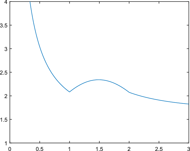
Note that $M_G(0.5)=3.0415$, $M_G(1)=2.0820$, $M_G(1.5)=2.3409$ and $M_G(2)=2.0741$, which reveal clearly that G does not possess the IDMTTF property. The MTTF function of G is displayed in Figure 1.

Figure 1.

MTTF function of G.

The next example illustrates that the mixture of two IDMTTF distributions need not be IDMTTF.

Example 3. Consider the life distribution given by the survival function

\begin{equation*}\bar{H}(x)=\dfrac{1}{2} \big\lbrace\skew3\bar{F}_1(x)+\skew3\bar{F}_2(x) \big\rbrace .\end{equation*}

This is a mixture of the survival functions $\skew3\bar{F}_1(x)$ defined in (13) and $\skew3\bar{F}_2(x)$ defined by

\begin{equation*} \skew3\bar{F}_2(x)=\begin{cases}\dfrac{1}{(1+x)} & 0<x\leq 1,\\[7pt]\dfrac{1}{2}\,{\textrm{e}}^{{{(x-1)}/{2}}} & 1\leq x < 2, \\[7pt]\dfrac{1}{2}\,{\textrm{e}}^{-{{x^2}/{8}}} & x \geq 2.\end{cases}\end{equation*}

Mitra and Basu [Reference Mitra and Basu42] showed that $F_2$ is a BFR distribution (see Definition 5 below) and every $x \in [1, 2]$ is a change point of $F_2$. Again Izadi et al. [Reference Izadi, Sharafi and Khaledi26] showed that the BFR class is contained in the IDMTTF class of life distributions. Consequently $F_2$ is a member of the IDMTTF class having change point $\tau=2.52914$. As already mentioned in Example 2, $\skew3\bar{F}_1(x)$ is IDMTTF with change point $\tau=1.7389$. Now the MTTF function corresponding to H is given by

\begin{equation*}M_H(x)=\dfrac{1}{H(x)}\int_0^{x} \bar{H}(u)\,{\textrm{d}} u.\end{equation*}

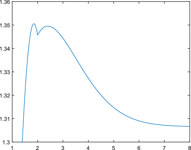
Here the values $M_H(1.85)=1.3505$, $M_H(2)=1.3456$, $M_H(2.5)=1.3494$ and $M_H(7.5)=1.3068$ clearly indicate that H is not IDMTTF. The MTTF function of H is plotted in Figure 2.

Figure 2.

MTTF function of H.

At this juncture we present an interesting observation in the following theorem, though it is somewhat outside the main focus of this section.

Proof. The equilibrium distribution of F is given by

\begin{equation*} F_{(1)}(t)=\dfrac{1}{\mu}\int_0^t \skew3\bar{F}(u) \,{\textrm{d}} u. \end{equation*}

Then its reversed hazard rate $r_{F_{(1)}}(t)$ equals

\begin{equation*} \dfrac{\skew3\bar{F}(t)}{\int_0^t \skew3\bar{F}(u) \,{\textrm{d}} u}. \end{equation*}

Now the MTTF function of F can be written as

\begin{equation*}M_F(t)=\dfrac{\int_0^t \skew3\bar{F}(u) \,{\textrm{d}} u}{F(t)}=\dfrac{\skew3\bar{F}(t)/F(t)}{r_{F_{(1)}}(t)}.\end{equation*}

The theorem follows easily using the fact that $\skew3\bar{F}(t)/F(t)$ is decreasing and F is IMTTF.

Now we shall attempt to study the interrelationships between various notions of non-monotonic ageing, namely the BFR class of Glaser [Reference Glaser23], the IDMRL class of Guess et al. [Reference Guess, Hollander and Proschan24], the NWBUE class of Mitra and Basu [Reference Mitra and Basu41] and the IDMTTF class of Izadi et al. [Reference Izadi, Sharafi and Khaledi26]. Before proceeding further, we recapitulate the definitions of the above-mentioned non-monotonic ageing classes.

Definition 6. A life distribution F with a finite first moment is called an increasing then decreasing mean residual life (IDMRL) (decreasing then increasing mean residual life (DIMRL)) distribution if there exists a point $\tau \geq 0$ such that $e_F(t)$ is increasing (decreasing) on $[0, \tau)$ and decreasing (increasing) on $[\tau, \infty)$, where

(14) \begin{equation}e_{F}(t)\,{:}\,{\raise-1.5pt{=}}\, \mathbb{E}(X-t \mid X>t)=\begin{cases}\displaystyle\int_{t}^{\infty}\skew3\bar{F}(u)\,{\textrm{d}} u / \skew3\bar{F}(t) & \text{if $\skew3\bar{F}(t)>0$,} \\[7pt]0 & \text{otherwise}.\end{cases}\end{equation}

The point $\tau$ is referred to as a change point (or turning point) of the distribution in the IDMRL (DIMRL) sense.

Mitra and Basu [Reference Mitra and Basu41] proved that the NWBUE family of life distributions is strictly larger than both IDMRL and BFR classes. An analogous chain of implications holds for the dual classes, i.e. $\{\textrm{UBFR}\} \subset \{\textrm{NBWUE}\}$ and $\{\textrm{DIMRL}\} \subset \{\textrm{NBWUE}\}$. Izadi et al. [Reference Izadi, Sharafi and Khaledi26] showed that $\{\textrm{BFR}\} \subset \{\textrm{IDMTTF}\} \subset \{\textrm{NWBUE}\}$ and $\{\textrm{UBFR}\} \subset \{\textrm{DIMTTF}\} \subset \{\textrm{NBWUE}\}$. We now explore the relation between the BFR and IDMRL classes of distributions using the total time on test (TTT) transform as a tool.

The scaled TTT transform of a life distribution F is defined by

\begin{align*}\psi_F(u)=\dfrac{\int_0^{F^{-1}(u)}\skew3\bar{F}(x) \,{\textrm{d}} x}{\mu}, \quad u\in[0,1],\\[-18pt]\end{align*}

where $F^{-1}(u)=\inf \lbrace x\colon F(x)\geq u \rbrace$. The TTT transform plays an important role in characterizing ageing classes of life distributions. Our goal is to show that the BFR class is contained in the IDMRL family of life distributions. To this end, we first recall the following two characterization theorems of Deshpande and Suresh [Reference Deshpande and Suresh16].

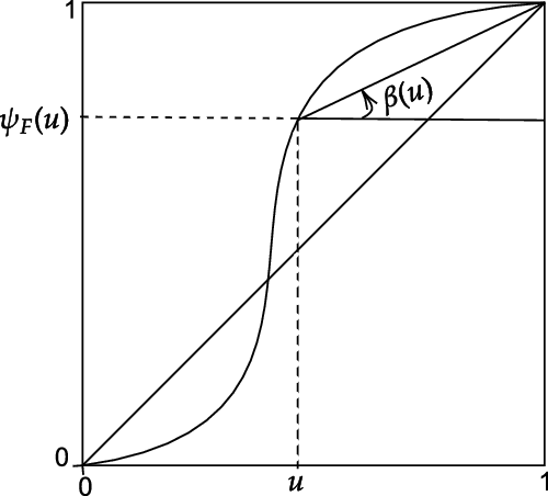
Figure 3 shows the plot of the scaled TTT transform of a distribution which is both IDMTTF and BFR. Geometrically, from Theorem 15, a distribution is IDMRL if and only if the angle $\beta(u)$ is increasing and then decreasing on (0, 1). We next prove a key lemma which will be useful in establishing the main result.

Figure 3.

Scaled TTT transform of a distribution which is BFR, IDMTTF and IDMRL.

Lemma 4. Let $x^*,x^{**}\in [0,1)$ and $f\colon [x^*,x^{**}]\rightarrow \mathbb{R}^+$ be a convex function on $[x^*,x^{**}]$. Suppose $S_f= \lbrace a \colon f(x)-1+a-ax=0 \,\, \text{has at least one root in} \,\, [x^*,x^{**}] \rbrace$. Now define

\begin{align*} \Tilde{a} & =\max S_f,\\*[3pt] \Tilde{x}_1 & =\min \lbrace x \colon \textit{\textit{x} is the root of $ f(x)-1+\Tilde{a}-\Tilde{a}x=0 $ in $ [x^*,x^{**}]$} \rbrace,\\[3pt] \Tilde{x}_2 & =\max \lbrace x \colon \textit{\textit{x} is the root of $ f(x)-1+\Tilde{a}-\Tilde{a}x=0$ in $ [x^*,x^{**}]$} \rbrace. \end{align*}

1. (i) If $\,\Tilde{x}_2=x^{**}$, then ${{(1-f(x))}/{(1-x)}}$ is increasing on $[x^*, x^{**})$.

2. (ii) If $\,\Tilde{x}_1=x^*$, then ${{(1-f(x))}/{(1-x)}}$ is decreasing on $(x^*,x^{**}]$.

3. (iii) If $x^*<\Tilde{x}_1\leq \Tilde{x}_2<x^{**}$, then ${{(1-f(x))}/{(1-x)}}$ is increasing on $[x^*,\Tilde{x})$ and decreasing on $[\Tilde{x},x^{**}]$ where $\Tilde{x}$ is any value in $[\Tilde{x}_1, \Tilde{x}_2]$.

Proof. It is easy to see that $S_f$ is a non-empty set. We now prove this lemma by contradiction.

1. (i) Suppose that ${{(1-f(x))}/{(1-x)}}$ is not increasing on $[x^*,x^{**})$. Then there exists $x_1,x_2$ such that $x^*\leq x_1 < x_2 < x^{**}$ and

   \begin{equation*} a_1=\frac{1-f(x_1)}{1-x_1}>\frac{1-f(x_2)}{1-x_2}=a_2. \end{equation*}
   Now convexity of f implies that
   \begin{equation*}\dfrac{a_2(1-x_2)-(1-f(\Tilde{x}_2))}{\Tilde{x}_2-x_2}=\dfrac{f(\Tilde{x}_2)-f(x_2)}{\Tilde{x}_2-x_2}\geq \dfrac{f(\Tilde{x}_2)-f(x_1)}{\Tilde{x}_2-x_1}> \dfrac{a_2(1-x_1)-(1-f(\Tilde{x}_2))}{\Tilde{x}_2-x_1}.\end{equation*}
   Some lengthy algebraic calculations now yield ${{(1-f(\Tilde{x}_2))}/{(1-\Tilde{x}_2)}}<a_2$, i.e. $\Tilde{a}<a_2$. This contradicts the definition of $\Tilde{a}$.

2. (ii) Suppose that ${{(1-f(x))}/{(1-x)}}$ is not decreasing on $(x^*,x^{**}]$. Then there exists $x_1,x_2$ such that $x^*< x_1 < x_2 \leq x^{**}$ and

   \begin{equation*}a_1=\frac{1-f(x_1)}{1-x_1}<\frac{1-f(x_2)}{1-x_2}=a_2.\end{equation*}
   Now convexity of f yields that
   \begin{equation*}\dfrac{a_1(1-x_1)-(1-f(\Tilde{x}_1))}{\Tilde{x}_1-x_1}=\dfrac{f(\Tilde{x}_1)-f(x_1)}{\Tilde{x}_1-x_1}\leq \dfrac{f(\Tilde{x}_1)-f(x_2)}{\Tilde{x}_1-x_2} < \dfrac{a_1(1-x_2)-(1-f(\Tilde{x}_1))}{\Tilde{x}_1-x_2}.\end{equation*}
   Algebraic manipulations now yield ${{(1-f(\Tilde{x}_1))}/{(1-\Tilde{x}_1)}}<a_1$, i.e. $\Tilde{a}<a_1$. Once again we arrive at a contradiction to the definition of $\Tilde{a}$.

3. (iii) The result follows by applying parts (i) and (ii) to $[x^*,\Tilde{x}_1]$ and $[\Tilde{x}_1, x^{**}]$, respectively, and also applying parts (i) and (ii) to $[x^*,\Tilde{x}_2]$ and $[\Tilde{x}_2, x^{**}]$, respectively.

Proof. As F is BFR, Theorem 14 guarantees the existence of $u_0\in [0,1]$ such that $\psi_F(u)$ is convex on $[0,u_0)$ and concave on $[u_0,1]$.

Case I: $u_0=0$. In this case $\psi_F(u)$ is concave on [0, 1], i.e. F is IFR and hence F is DMRL. So F is IDMRL with change point $\tau=0$.

Case II: $u_0=1$. In this case $\psi_F(u)$ is convex on [0,1), i.e. F is DFR and hence F is IMRL. So F is IDMRL with a change point at infinity.

Case III: $0<u_0<1$. Lemma 2.1 of Suresh [Reference Suresh51] shows that the mean residual life (MRL) function $e_F(t)$ is decreasing for $t\geq F^{-1}(u_0)$. Now it is easy to show that ${{(1-\psi_F(u))}/{(1-u)}}$ is decreasing on $[u_0,1)$ using an argument similar to the one in the proof of Theorem 2.5 of Klefsjö [Reference Klefsjö32]. Note that using a slight modification of the arguments in the proof of Theorem 3.2 in Deshpande and Suresh [Reference Deshpande and Suresh16], we conclude that $\psi_F(u)$ is a convex, positive function on $[0,u_0]$. Now in Lemma 4, we take $f=\psi_F$, $x^*=0$ and $x^{**}=u_0$.

Subcase i: $0<\Tilde{x}_1\leq \Tilde{x}_2<u_0$. By (iii) in Lemma 4, there exists $\Tilde{u}\in [x^*, x^{**}]=[0,u_0]$ such that ${{(1-\psi_F(u))}/{(1-u)}}$ is increasing on $[0,\Tilde{u})$ and decreasing on $[\Tilde{u}, u_0]$. Now applying Theorem 15 we get that F is IDMTTF with change point $\tau=F^{-1}(\Tilde{u})$.

Subcase ii: $\Tilde{x}_1=0=x^*$. By (ii) in Lemma 4, we get that ${{(1-\psi_F(u))}/{(1-u)}}$ is decreasing in $(0,u_0]$. Hence ${{(1-\psi_F(u))}/{(1-u)}}$ is decreasing in [0,1). Now Theorem 2.5 of Klefsjö [Reference Klefsjö32] shows that F DMRL, i.e. F is IDMRL with change point $\tau=0$.

Subcase iii: $\Tilde{x}_2=x^{**}=u_0$. By (i) in Lemma 4, we get that ${{(1-\psi_F(u))}/{(1-u)}}$ is increasing in $[0,u_0)$. Hence applying Theorem 15 we get that F is IDMRL with change point $\tau=F^{-1}(u_0)$.

In all the above cases $\Tilde{u}\leq u_0$, i.e. $\tau\leq t_0$, which completes the proof.

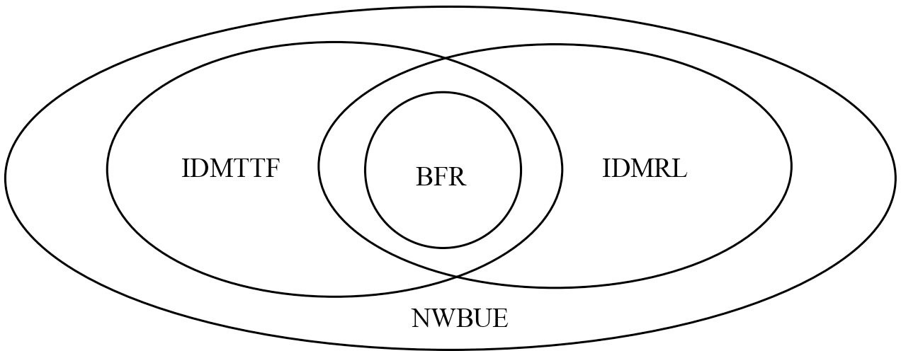
Thus the IDMTTF and IDMRL classes both contain the BFR family of life distributions and are contained in the NWBUE class. A natural question arises: Does any one of the IDMTTF and IDMRL properties imply the other? The following two examples answer this question in the negative.

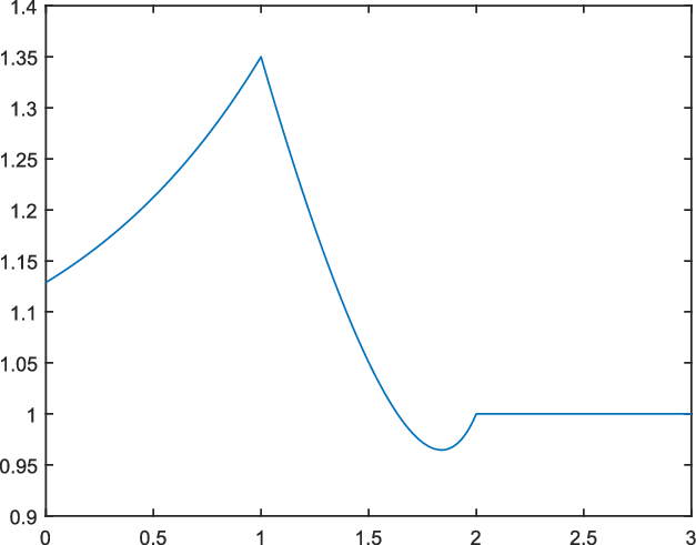
Example 4. Consider the IDMTTF distribution given by the survival function $\skew3\bar{F}_1$ in (13). Denoting the MRL function of $F_1$ by $e_{F_1}(x)$, we have $e_{F_1}(0.5)=1.2123$, $e_{F_1}(1)=1.3500$, $e_{F_1}(1.8)=0.9662$ and $e_{F_1}(2.5)=1$, which clearly demonstrate that $F_1$ does not possess the IDMRL property. The MRL function of $F_1$ is plotted in Figure 4.

Figure 4.

MRL function of $F_1$.

Example 5. Consider the life distribution given by the following survival function:

\begin{equation*} \bar{G}(x)=\begin{cases}\dfrac{1}{(1+x)^2} & 0<x\leq 1,\\ \\[-7pt]\dfrac{ {\textrm{e}}^{(1-x)/2x}}{4x^2} & 1\leq x< 2, \\ \\[-7pt]\dfrac{18-x}{2^8 \,{\textrm{e}}^{1/4}} & 2\leq x< 10, \\ \\[-7pt]\dfrac{(6-{{x}/{5}})^4}{2^{13} \,{\textrm{e}}^{1/4}} & 10\leq x < 25, \\ \\[-7pt]\dfrac{ {\textrm{e}}^{3/4}}{2^{13}}\,{\textrm{e}}^{x-25- {\textrm{e}}^{x-25}} & x \geq 25.\end{cases}\end{equation*}

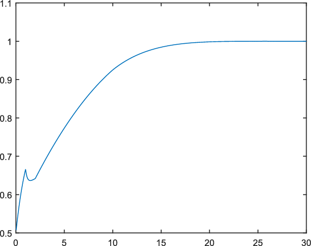
Anis [Reference Anis5] showed that G is IDMRL with change point 2. Now the MTTF function of G is denoted by $M_G(x)$. Note that $M_G(0.9)=0.6552$, $M_G(1.5)=0.6366$, $M_G(2)=0.6418$ and $M_G(9)=0.9015$, which clearly indicate that G does not have the IDMTTF property. Figure 5 shows the MTTF function of G.

Figure 5.

MTTF function of G.

Figure 6.

The relationships between certain non-monotonic classes of life distributions.

Combining our findings together with the results of Izadi et al. [Reference Izadi, Sharafi and Khaledi26] and Mitra and Basu [Reference Mitra and Basu41], we provide in Figure 6 diagrammatic representation of interrelationships between the BFR, IDMRL, IDMTTF and NWBUE classes of life distributions.

Using analogous arguments, similar diagrammatic representation of interrelationships between the UBFR, DIMRL, DIMTTF and NBWUE classes of life distributions can be obtained.