


1. Introduction
Preferential attachment graphs (PAGs) form a group of random growing graph models that have been studied for a long time ([Reference Barabási and Albert2], [Reference Durrett9], and [Reference Frieze and Karoński12]). The main motivation is modelling randomly evolving large real-world networks, such as online and offline social networks, the internet, or biological networks (e.g. protein–protein interactions). The basic PAG models have been extended by various features, for example duplication steps, weighted edges, vertices with random fitness. The study of this wide family of models provided information about several phenomena in real-world networks (asymptotic degree distribution, clustering, relation of local and global properties, epidemic spread). The limiting behaviour of PAG models has also been investigated from various points of view, depending somewhat on the edge density along the graph sequences. For instance, in [Reference Berger, Borgs, Chayes and Saberi3], Berger, Borgs, Chayes, and Saberi consider a sparse version of the process, with a linear number of edges compared to the number of vertices, and prove convergence in the sense of Benjamini and Schramm to a Pólya point graph. A variation with added randomness is considered by Elwes in [Reference Elwes10] and [Reference Elwes11], where the preferential attachment model is amended in such a way that the number of edges added at each stage itself is a random variable, but in expectation still preserves linear growth. The limit here is the infinite Rado graph, or a multigraph variant of the same, depending on whether multiple edges are allowed during the process.
At the dense end of the spectrum, when the edge density along the sequence is essentially constant c (i.e. the number of edges is approximately cn 2/2), the PAG model corresponds to a Pólya urn model where each urn starts with one ball in it. If, instead of speaking of the number of balls in each urn, we speak of the ‘weight’ of an urn, it becomes natural to consider an initial state with each weight being equal to a parameter κ ∊ (0, ∞) (restricting to equal weights preserves symmetry and exchangeability), giving rise to the so-called PAG κ model (see [Reference Ráth and Szakács17]).
Borgs, Chayes, Lovász, Sós, and Vesztergombi [Reference Borgs, Chayes, Lovász, Sós and Vesztergombi6] considered the model PAG1 under the convergence notion of injective graph densities. They showed that with probability 1 the graph sequence converges to the graphon W :[0, 1]2 → ℝ given by W(x, y) = c ln x ln y. Later, Ráth and Szakács considered in [Reference Ráth and Szakács17] convergence of a more general family of processes with respect to induced multigraph densities, showing that the limit object of the PAG κ model is a graphon that now takes Poisson distributions as values instead. Hence the corresponding graphs (generated randomly from this limit object) contain multiple edges with no uniform upper bound on the multiplicity, and the original notions for limits of simple graphs cannot be used any longer. The paper [Reference Kunszenti-Kovács, Lovász and Szegedy14]by Kunszenti-Kovács, Lovász, and Szegedy provides a framework for handling homomorphism densities in the context of multigraphs, and makes use of the so-called jumble norm to measure distance between graphons.
All of the papers [Reference Borgs, Chayes, Lovász, Sós and Vesztergombi6], [Reference Kunszenti-Kovács, Lovász and Szegedy14], and [Reference Ráth and Szakács17] also deal with W-random graph sequences induced by the limit objects W, and show that with probability 1, the resulting graph sequence converges to W in the respective densities sense. These W-random graph models are thus very similar to the classical graph sequences that gave rise to the limit W, but also exhibit some significant differences.
The specific models we work with are the following. First, we fix two constants c,κ > 0.
Definition 1. We choose independent random variables ξ
i
with gamma(κ, κ) distribution for every 1 ≤ i ≤ n.For i < j, let Y
ij
be a Poisson random variable with parameter cξ
i
ξ
j
. For every i, let Y
ii
be a Poisson random variable with parameter
 $$c\xi _i^2/2$$
. Assume that all Y
ij
are conditionally independent with respect to the ξ
i
. We put Y
ij
edges between vertices i and j for every 1 ≤ i ≤ j ≤ n. We obtain the random multigraph
 $${\mathbb {G}}_{\rm{W}}^ \circ (n)$$
in this way.
If, compared to
 $${\mathbb {G}}_{\rm{W}}^ \circ (n)$$
, we do not add the loops (i.e. we set Y
ii
≡ 0 for all i), we obtain the random multigraph 𝔾W(n).
Remark. Note that using gamma variables instead of the uniform [0, 1]-valued ones is compensated by the loss of F −1 in the parameter.
These are the random models we wish to compare to the following version of the PAG model.
Definition 2. Given vertices {1, 2,..., n}, we assign an urn to each vertex, initially with one single ball in each of them. Then we run a linear Pólya urn process for 2˪cn 2/2⌋ steps. That is, at each step we choose an urn with probabilities proportional to κ plus the actual number of balls, and put an extra ball into it. More precisely, for t = 1, 2,..., 2˪cn 2/2⌋, at step t, an urn containing d balls is chosen with probability
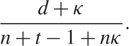 $${{d + \kappa } \over {n + t - 1 + n\kappa }}.$$
Then we put a new ball into this urn (each random choice is conditionally independent of the previous steps, given the actual distribution of the balls). Finally, for k = 1, 2,..., ˪cn 2/2⌋, we add an edge between the vertices where the balls at step t = 2k − 1 and at step t = 2k have been placed. We obtain a random multigraph 𝔾PAG(n) in this way; multiple edges and loops may occur.
To compare these models, we shall use the following distance notion between multigraphs. It may be defined more generally for graphons (which essentially are weighted graphs with vertex set [0, 1]), but that will not be needed here, and we refer to [Reference Kunszenti-Kovács, Lovász and Szegedy14] for more details.
Definition 3. Let G and H be two (multi-)graphs on the same vertex set [n]≔{1,..., n} for some positive integer n. Then we define their jumble-norm distance as
 $${d_\otimes}(G,H) = {1 \over n} \cdot \mathop {\max }\limits_{S,T \subseteq [n]} {1 \over {\sqrt {|S| \cdot |T|} }}|\sum\limits_{i \in S,j \in T} {U_{ij}} - {V_{ij}}|,$$
where U ij and V ij denote the multiplicity of edge ij in G and H, respectively.
Our goal in this paper is to show that with probability 1 they are close (but not too close) in the jumble distance. This result can be interpreted as an upper bound on the speed of convergence of the PAG κ model, in the sense that it is compared to a finite version of the limit object, and not to the graphon itself. Specifically, we have the following main result.
Theorem 1. Given κ and c, there exist K > 0 and a coupling of the preferential attachment model and the W-random graph on n vertices such that for every n ≥ 1 we have
 $$\mathbb {E}({d_\otimes}({\mathbb {G}_{{\rm{PAG}}}}(n),{\mathbb {G}}_{\rm{W}}(n))) \le K \cdot \mathop {\log }\nolimits^{3/2} n \cdot {n^{ - 1/2}}.$$
The idea of the proof of the main result is to define a coupling based on a Poisson process, which connects the W-random graph and the PAG κ model (see Section 3). The proofs can be found in Section 4. In the discussion part (Section 5), we point out some features of the W-random version that can make it more useful in certain applications.
2. Motivation
It was proved in [Reference Kunszenti-Kovács, Lovász and Szegedy14] that with probability 1, the random graph
 $${\mathbb {G}}_{\rm{W}}^ \circ (n)$$
converges to the original function W with respect to multigraph homomorphism densities. As mentioned, this is also the limit object of the sequence of the preferential attachment random graphs 𝔾PAG(n) with parameter κ on n vertices with ⌋cn
2⌋ edges. Given that letting n go to infinity, the two random sequences 𝔾PAG(n) and
 $${\mathbb {G}}_{\rm{W}}^ \circ (n)$$
tend to the same limit, it is natural to ask how close these two sequences are as a function of n.
In this section we shall go into more detail about the specific choices made concerning the objects and properties studied. For limits of simple graphs, or even graphs with a uniform bound on the edge multiplicity, the standard distance notion used is that of the cut norm. The cut-norm distance d
⃛ used in many other papers (see e.g. [Reference Borgs, Chayes, Lovász, Sós and Vesztergombi6] for details) differs from the jumble-norm distance d
⊠ in the factor
 $$1/\sqrt {|S| \cdot |T|} $$
that is omitted in the former. As such, our current distance notion magnifies the differences that occur on small sets, and we clearly have d ⊠ ≥ d ⃛. The jumble-norm distance turns out to be a more useful tool when introducing a metric for generalized graphons, in part due to the fact that it can be considered as an L
2-version of the cut-norm distance (since
 $$\sqrt {|S| \cdot |T|} $$
corresponds to the L
2-norm of the characteristic function of the set S × T), leading to simpler expressions for bounds (cf. [Reference Borgs, Chayes, Cohn and Lovász5] and [Reference Kunszenti-Kovács, Lovász and Szegedy14]).
Next, we turn our attention to Definition 1, and our choice of distribution for the variables ξ i . Whilst the first parameter κ does very much influence the model, it is not clear why the second parameter has to be identical. Indeed it is not necessary, but we shall explain why this particular choice was made, and why no loss of generality incurs.
Let ℳ denote the space of finite measures on ℕ, and let W :[0, 1]2 → ℳ be the function given by
 $$W(x,y) = {\mu _{c{F^{ - 1}}(x){F^{ - 1}}(y)}},$$
where
 $$F(z) = \int_0^z {1 \over {\Gamma (\kappa )}}{\kappa ^\kappa }{t^{\kappa - 1}}{{\rm{e}}^{ - \kappa t}}{\rm{d}}t$$
is the CDF of gamma(κ, κ) and μ λ denotes the Poisson distribution with parameter λ.
This is the graphon that represents the limit of the 𝔾PAG(n) sequence, and is well-defined fixing κ and c. Now the natural way of generating the so-called W-random graph model from it is as follows. We consider the set [0, 1] as the vertex set of the infinite graph with ‘adjacency function’ W, and sample a random spanned subgraph on n vertices by choosing its vertices independently uniformly from [0, 1]. After this first randomization, we obtain a ‘graph’ on n vertices where each ‘edge’ is a Poisson distribution (or, equivalently, each pair of not necessarily different vertices is labelled with the appropriate Poisson distribution). To obtain a true multigraph, we then independently sample an edge multiplicity for each pair of different vertices from the corresponding Poisson distribution. As for pairs of identical vertices, if we allow loops, for technical reasons we first halve the parameter of the Poisson distribution, then double the sampled value (in this way the graphon takes a simpler form; typically changing W on a set of measure zero does not influence densities if the test-graphs are loopless). This will correspond to the random graph
 $${\mathbb {G}}_{\rm{W}}^ \circ (n)$$
, whereas if loops are disallowed, we obtain the random graph 𝔾
W
(n).
Note that changing the scale parameter for the ξ i will not change anything: as the values of W(x, y) do not change, it would merely render the conversion from W to the model in Definition 1 more complicated, hence our choice of keeping the two parameters equal. As an added bonus, the distributions (κ, κ) all have expected value 1, simplifying the computations (and this is certainly also the reason for the specific choice of distributions used in the formula of W in [Reference Ráth and Szakács17]).
In the last section, we provide a universal, coupling-independent lower bound of Θ (n −1/2) for the same expectation. The exponents match, but the logarithmic term still leaves room for improvement.
3. Coupling
In order to prove Theorem 1, we need to construct a particular coupling for which the distance of 𝔾PAG and 𝔾W is smaller than the upper bound. We build a coupling of appropriate realizations of 𝔾PAG and
 $${\mathbb {G}}_{\rm{W}}^ \circ $$
, then we find a realization of 𝔾W in the same probability space.
We will use the following well-known fact (which can also be considered as an application of de Finetti’s theorem on exchangeable random variables). Let
 $$({\xi _i})_{i = 1}^n$$
be independent gamma(κ, κ)-distributed random variables, as in Definition 1. We consider N random variables that are independent and identically distributed conditionally with respect to
 $$({\xi _i})_{i = 1}^n$$
, and each of them takes value i with probability
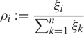 $${\rho _i}{\kern 1pt} : = {{{\xi _i}} \over {\sum\limits_{k = 1}^n {\xi _k}}}$$
for i = 1, 2,..., n. Then we get the joint distribution of the sequence of the first N draws of the n-colour Pólya urn. Indeed, these N random variables have a Dirichlet joint distribution (see e.g. [Reference Devroye8, Theorem XI.4.1.]), and using the moments of Dirichlet distributions, it can be seen that this distribution is the same as the joint distribution of the first N draws (see [Reference Blackwell and Macqueen4], [Reference Degroot7], or [Reference Wong18, Section 2]).
We construct the coupling based on a sequence of independent random variables
 $$({\xi _i})_{i = 1}^n$$
with distribution gamma(κ, κ). Conditionally with respect to
 $$({\xi _i})_{i = 1}^n$$
, we assign independent Poisson processes to each pair of vertices. For 1 ≤ i < j ≤ n, the rate of the process is 2ρ
i
ρ
j
for the pair (i, j) (with ρ
i
defined above), and for 1 ≤ i ≤ n, the rate is
 $${\rho _i}^2$$
for (i, i). We denote by
 $$N_s^{(ij)}$$
the number of events until time s in the process assigned to (i, j). The cumulation of these processes is also a Poisson process. Let τ be the time when the total number of events reaches ⌋cn
2/2⌋. We get a realization of 𝔾PAG(n) if we put
 $$N_\tau ^{(ij)}$$
edges between i and j for all 1 ≤ i ≤ j ≤ n. Indeed, all ⌋cn
2/2⌋ events are distributed among the pairs of vertices independently, with probabilities proportional to the rates 2ρ
i
ρ
j
and
 $$\rho _i^2$$
. Thus this is the same as the joint distribution of consecutive pairs of 2⌋cn
2/2⌋ independent elements chosen according to
 $$({\rho _i})_{i = 1}^n$$
, which provides a Pólya urn by the argument above. On the other hand, we get a realization of
 $${\mathbb {G}}_{\rm{W}}^ \circ (n)$$
if we put
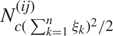 $$N_{c{{(\sum\nolimits_{k = 1}^n {\xi _k})}^2}/2}^{(ij)}$$
edges between i and j, because the number of edges between the pairs of vertices are independent Poisson random variables with the appropriate parameters:
 $${1 \over 2}c{(\sum\limits_{k = 1}^n {\xi _k})^2} \cdot 2{\rho _i}{\rho _j} = c{\xi _i}{\xi _j}\quad {\rm{and}}\quad {1 \over 2}c{(\sum\limits_{k = 1}^n {\xi _k})^2} \cdot \rho _i^2 = c\xi _i^2/2.$$
Hence this provides a coupling of the two models.
Proposition 1. In the coupling above, for some K 1,2 > 0 we have
 $$\mathbb {E}({d_\otimes}({\mathbb {G}_{{\rm{PAG}}}}(n),\mathbb {G}_W^ \circ (n))) \le {K_{1,2}} \cdot {n^{ - 1/2}} \cdot \mathop {\log }\nolimits^{3/2} n,\quad \quad n = 1,2, \ldots .$$
As for 𝔾
W
(n), we can use the same probability space as before, generate
 $${\mathbb {G}}_{\rm{W}}^ \circ (n)$$
, and then delete the loops.
Proposition 2. There exists K 2,3 > 0 such that
 $$\mathbb {E}({d_\otimes}(\mathbb {G}_W^ \circ (n),{\mathbb {G}_W}(n))) \le {K_{2,3}} \cdot {n^{ - 3/4}},\quad \quad n = 1,2, \ldots $$
holds when 𝔾
W
is obtained from
 $${\mathbb {G}}_{\rm{W}}^ \circ (n)$$
by deleting the loops.
4. Proofs
Proof of Theorem 1. The statement follows from Propositions 1 and 2.
We shall therefore now turn our attention to proving the bounds connecting each pair of models. Since the jumble-norm distance is not always easy to work with, we shall make use of the following lemma.
Lemma 1. Let G and H be two (undirected) multigraphs on the vertex set {1, 2,..., n}. Let Uij be the number of edges between i and j in G, and Vij the same quantity in H. Then the following holds:
 $${d_n}(G,H) = \frac{1}{n} \cdot \mathop {\max }\limits_{S,T} \frac{1}{{\sqrt {|S| \cdot |T|} }}|\sum\limits_{i \in S,j \in T} {{U_{ij}}} - {V_{ij}}| \le \frac{1}{n} \cdot \mathop {\max }\limits_{1 \le i \le n} \;\sum\limits_{j = 1}^n | {U_{ij}} - {V_{ij}}|.$$
Proof. Let
 $${\sigma _i} = \sum\nolimits_{j = 1}^n |{U_{ij}} - {V_{ij}}|$$
. Notice that if |S| = s, |T| = t, and s ≤ t, then
 $$|\sum\limits_{i \in S,j \in T} {U_{ij}} - {V_{ij}}| \le \sum\limits_{i \in S,j \in T} |{U_{ij}} - {V_{ij}}| \le \sum\limits_{i \in S} {\sigma _i} \le s\mathop {\max }\limits_{1 \le i \le n} {\sigma _i}.$$
Hence
 $$\frac{1}{{\sqrt {st} }}|\sum\limits_{i \in S,j \in T} {{U_{ij}}} - {V_{ij}}| \le \frac{{s{{\max }_{1 \le i \le n}}{\sigma _i}}}{{\sqrt {st} }} = \frac{{\sqrt s }}{{\sqrt t }}\mathop {\max }\limits_{1 \le i \le n} {\sigma _i} \le \mathop {\max }\limits_{1 \le i \le n} {\sigma _i},$$
as we assumed that s ≤ t. In the reverse case s ≥ t, we get the same with the bound
 $$\mathop {\max }\limits_{1 \le j \le n} \sum\limits_{i = 1}^n |{U_{ij}} - {V_{ij}}|.$$
Since U ij = U ji and V ij = V ji , this is equal to the previous maximum. This finishes the proof.
4.1. Models 𝔾PAG and
 $${\mathbb {G}}_{\rm{W}}^ \circ $$

Proof of Proposition 1. Let U
ij
be the number of edges between i and j in the random graph 𝔾PAG, and let V
ij
be the number of edges between them in model
 $${\mathbb {G}}_{\rm{W}}^ \circ $$
. By using the notations introduced for the coupling of the two models, we have
 $${U_{ij}} - {V_{ij}} = N_\tau ^{(ij)} - N_\sigma ^{(ij)}$$
where
 $$\sigma = c{(\sum\nolimits_{k = 1}^n {\xi _k})^2}/2$$
. If τ ≥ σ, then all these differences are nonnegative, and all of them are negative if τ <σ. Thus
 $${\Delta _{n,i}} = \sum\limits_{j = 1}^n |{U_{ij}} - {V_{ij}}| = |\sum\limits_{j = 1}^n N_\tau ^{(ij)} - N_\sigma ^{(ij)}|,\quad \quad 1 \le i \le n.$$
We will use the fact that by cumulating the independent Poisson processes assigned to the pairs of vertices we get a Poisson process with rate
 $$2\sum\nolimits_{i \lt j} {\rho _i}{\rho _j} + \sum\nolimits_i \rho _i^2 = 1$$
. Let N
s
be the total number of events until time s, that is,
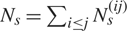 $${N_s} = \sum\nolimits_{i \le j} N_s^{(ij)}$$
, which has Poisson distribution with parameter s. Since there are |⌋cn
2/2⌋ events in the cumulated process until τ, there are |⌋cn
2/2⌋ − N
σ
| events between τ and σ. On the other hand, independently of each other, all these events increase Δ
n,i
by 1 with probability p
i
= ρ
i
(ρ
i
+ 2 Σj≠i ρ
j
) ≤ 2ρ
i
, because we can think of the process as the cumulated Poisson process with the types of the events chosen independently with probabilities proportional to the rates. We conclude that, conditionally with respect with respect to N
σ
and
 $$({\xi _i})_{i = 1}^n$$
, the quantity Δ
n,i
has binomial distribution with parameters |⌋cn
2/2⌋ − N
σ
| and p
i
.
We will give an upper bound on Δ
n,i
on an appropriately chosen event which has large probability. First, since each ξ
i
is a random variable with distribution gamma(κ, κ), and they are independent, the proportion
 $${\rho _i} = {\xi _i}/(\sum\nolimits_{k = 1}^n {\xi _k})$$
has distribution beta(1, n − 1).
Therefore, for n ≥ 2 we have
 $$\mathbb {P}\matrix{
{({\rho _i} > {{16} \over n}\log n)} \hfill & = \hfill & {\int_{16\log n/n}^1 (n - 1)(1 - x{)^{n - 2}}{\kern 1pt} {\rm{d}}{\kern 1pt} x} \hfill \cr
{} \hfill & = \hfill & {\int_0^{1 - 16\log n/n} (n - 1){x^{n - 2}}{\kern 1pt} {\rm{d}}{\kern 1pt} x} \hfill \cr
{} \hfill & = \hfill & {{{(1 - 16\log n/n)}^{n - 1}}} \hfill \cr
{} \hfill & \le \hfill & {\exp ( - 8\log n)} \hfill \cr
{} \hfill & = \hfill & {{n^{ - 8}}.} \hfill \cr
} $$
Since
 $$({\xi _k})_{k = 1}^n$$
are independent and identically distributed random variables satisfying the conditions of Cramér’s theorem (or the Chernoff bound), we can choose a > 0 such that
 $${\mathbb {P}}(\sum\limits_{k = 1}^n {\xi _k} - n > a \cdot {n^{1/2}}\sqrt {\log n} ) = {\rm{O}}({n^{ - 8}})$$
holds. Below, we fix such an a, and define
 $${s_n} = c{n^2}/2 - 2ac{n^{3/2}}\sqrt {\log n} $$
and
 $${t_n} = c{n^2}/2 + 2ac{n^{3/2}}\sqrt {\log n} $$
. Then
 $${N_{{s_n}}}$$
and
 $${N_{{t_n}}}$$
have Poisson distributions with parameters s
n
and t
n
, respectively. By a standard application of Chernoff’s bound for these random variables, we find that there exists b > 0 such that
 $${N_{{s_n}}} - {s_n} \lt - bn\sqrt {\log n} $$
and
 $${N_{{t_n}}} - {t_n} > bn\sqrt {\log n} $$
both have probability O(n
−8).
The arguments above imply that we have
 $$\mathbb {P}({F_{n,i}}) \ge 1 - {\rm{O}}({n^{ - 8}}),$$
where we define
 $$\matrix{
{{F_{n,i}} = \{ {\rho _i} \le {{16} \over n}\log n\} \cap \{ |\sum\limits_{k = 1}^n {\xi _k} - n| \lt a \cdot {n^{1/2}}\sqrt {\log n} \} } \cr
{ \cap \{ {N_{{s_n}}} > {s_n} - bn\sqrt {\log n} \} \cap \{ {N_{{t_n}}} \lt {t_n} + bn\sqrt {\log n} \} .} \cr
} $$
Now we will bound Δ n,i on this event F n,i (for fixed i). Notice that (for sufficiently large n) the second condition in this definition implies that
 $$|(\sum\limits_{k = 1}^n {\xi _k}{)^2} - {n^2}| \le a{n^{1/2}}\sqrt {\log n} \cdot (2n + a{n^{1/2}}\sqrt {\log n} ),$$
and thus
 $${s_n} \le \sigma = c{(\sum\nolimits_{k = 1}^n {\xi _k})^2}/2 \le {t_n}$$
. Therefore, for sufficiently large n, on the event F
n,i
we have
 $${N_\sigma } - c{n^2}/2 \ge {N_{{s_n}}} - c{n^2}/2 \ge {s_n} - bn\sqrt {\log n} - c{n^2}/2 \ge - 3ac{n^{3/2}}\sqrt {\log n} $$
and
 $${N_\sigma } - c{n^2}/2 \le {N_{{t_n}}} - c{n^2}/2 \le {t_n} + bn\sqrt {\log n} - c{n^2}/2 \le 3ac{n^{3/2}}\sqrt {\log n} ,$$
and consequently
 $$|{N_\sigma } - c{n^2}/2| \le 3ac{n^{3/2}}\sqrt {\log n} .$$
Recall that, conditionally with respect to
 $$({\xi _i})_{i = 1}^n$$
and N
σ
, the random variable Δ
n,i
has binomial distribution with parameters |N
σ
− ⌋cn
2/2⌋| and p
i
, which was at most 2ρ
i
≤ 32 log n/n on F
n,i
. Let ℱ be the σ-algebra generated by
 $$({\xi _i})_{i = 1}^n$$
and the process N. Then, since F
n,i
is measurable with respect to ℱ, we have
 $$\matrix{
{\mathbb {P}}{(\{ {\Delta _{n,i}} > 192ac \cdot {n^{1/2}}\mathop {\log }\nolimits^{3/2} n\} \cap {F_{n,i}})} \hfill \cr
{\quad \quad \le (({{{{\rm{e}}^{{\Delta _{n,i}}}}} \over {\exp (192ac \cdot {n^{1/2}}\mathop {\log }\nolimits^{3/2} n)}}|{\cal F}) \cdot {_{{F_{n,i}}}})} \hfill \cr
{\quad \quad = ({{{{(1 + (e - 1){p_i})}^{|{N_\sigma } - c{n^2}/2|}}} \over {\exp (192ac \cdot {n^{1/2}}\mathop {\log }\nolimits^{3/2} n)}} \cdot {_{{F_{n,i}}}})} \hfill \cr
{\quad \quad \le \exp ((e - 1)(32\log n/n) \cdot 3ac \cdot {n^{3/2}}\mathop {\log }\nolimits^{1/2} n - 192ac \cdot {n^{1/2}}\mathop {\log }\nolimits^{3/2} n)} \hfill \cr
{\quad \quad = {\rm{O}}({n^{ - 8}}).} \hfill \cr
} $$
Putting this together with equation (1) we conclude that
 $${\mathbb {P}}(\sum\limits_{j = 1}^n |{U_{ij}} - {V_{ij}}| > 192ac \cdot {n^{1/2}}\mathop {\log }\nolimits^{3/2} n) = {\rm{O}}({n^{ - 8}})$$
holds for every i with 1 ≤ i ≤ n.
Finally, let An
be the event that
 $$\sum\nolimits_{j = 1}^n |{U_{ij}} - {V_{ij}}| > 192ac \cdot {n^{1/2}}\mathop {\log }\nolimits^{3/2} n$$
holds for some 1 ≤ i ≤ n. This last inequality implies ℙ(An
) = O(n
−7). By using Lemma 1, the Cauchy–Schwarz inequality and the fact that Nσ
has Poisson distribution conditionally with respect to σ, we obtain
 $$192ac \cdot {n^{ - 1/2}}\mathop {\log }\nolimits^{3/2} n + {\rm{O}}({n^{ - 4}})(2({\sigma ^2} + \sigma + {c^2}{n^4}{))^{1/2}}.$$
This implies the statement if we calculate the moments of
 $$\sigma = c{(\sum\nolimits_{k = 1}^n {\xi _k})^2}/2$$
by using that the sum has gamma(nκ, κ) distribution, and hence its rth moment is
 $${{\Gamma (n\kappa + r)} \over {{\kappa ^r}\Gamma (n\kappa )}}.$$
4.2. Models
$${\mathbb {G}}_{\rm{W}}^ \circ $$
and 𝔾
W

Proof of Propositon 2. We note that
 $${\mathbb {G}}_{\rm{W}}^ \circ (n)$$
and 𝔾
W
(n) coincide everywhere but the main diagonal, and it is then easy to see that
 $${d_n}(_W^ \circ (n),{\mathbb {G}_W}(n)) = {1 \over n} \cdot \mathop {\max }\limits_{1 \le i \le n} {Y_{ii}}.$$
Recall that Yii
has Poisson distribution with parameter
 $$c\xi _i^2$$
, where ξi
has gamma(κ, κ) distribution. Assume first that ζ > 0 is fixed, and X ~ Pois(ζ ). Then
 $$\sum\limits_{k = y + 1}^\infty (X \ge k) \le \sum\limits_{k = y + 1}^\infty k(X = k) = \sum\limits_{k = y + 1}^\infty {{{\zeta ^k}} \over {(k - 1)!}}{\kern 1pt} {{\rm{e}}^{ - \zeta }} \le \zeta \sum\limits_{k = z}^\infty {{{\zeta ^k}} \over {k!}}{\kern 1pt} {{\rm{e}}^{ - \zeta }} = \zeta (X \ge y).$$
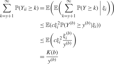
We will use the factorial moments of the Poisson distribution. We use the notation x (b) = x(x − 1) ⋯ (x − b + 1). For every fixed i and integers y > b > 0, we have
 $$\matrix{
{\sum\limits_{k = y + 1}^\infty ({Y_{ii}} \ge k)} \hfill & = \hfill & {((\sum\limits_{k = y + 1}^\infty (Y \ge k)|{\xi _i}))} \hfill \cr
{} \hfill & \le \hfill & {(c\xi _i^2({Y^{(b)}} \ge {y^{(b)}}|{\xi _i}))} \hfill \cr
{} \hfill & \le \hfill & {(c\xi _i^2{{\xi _i^{(b)}} \over {{y^{(b)}}}})} \hfill \cr
{} \hfill & = \hfill & {{{K(b)} \over {{y^{(b)}}}}} \hfill \cr
} $$
for some K(b) > 0, because the gamma distribution has finite moments.
For an arbitrary function f : ℕ+ → ℕ+ we may apply the above inequality to obtain
 $$(\mathop {\max }\limits_{1 \le i \le n} |{Y_{ii}}|) = \sum\limits_{k = 1}^\infty (\mathop {\max }\limits_{1 \le i \le n} |{Y_{ii}}| \ge k) \le f(n) + \sum\limits_{k = f(n) + 1}^\infty n({Y_{11}} \ge k) \le f(n) + n{{K(b)} \over {f{{(n)}^{(b)}}}}.$$
Now let N ∊ ℕ+ be fixed, set f (n) ≔ n 1/5 and b ≔ 4. For sufficiently large n (such that n − 3 ≥ n/2 and f (n)(4) ≥ f (n)4/16), this yields
 $${\mathbb {E}}(\mathop {\max }\limits_{1 \le i \le n} |{Y_{ii}}|) \le {n^{1/5}} + 16K(4){n^{1 - 4/5}} \le {n^{1/4}}(K(4) + 1)).$$
Lemma 1 concludes the proof.
5. Discussion
Our main theorem shows that the classical dense preferential attachment graph model yields random graphs that are close to the random graph model obtained through the PAG κ - graphon, the limit object in the multigraph homomorphism sense of the random sequence 𝔾PAG. They are not indistinguishable, however (we provide a lower bound on their distance below), and they each have their own advantages for applications.
The random graphs 𝔾PAG have the advantage that the number of edges is deterministic, but, contrary to the sparse PAG models, one cannot easily generate a growing family of graphs 𝔾PAG(n). For the graphon induced
 $${\mathbb {G}}_{\rm{W}}^ \circ $$
, the number of edges is random, though still asymptotically concentrated around the expected value. Also, the way it is generated does not carry the preferential attachment flavour. This may be an advantage from the simulation point of view: the random variables in the model can be generated simultaneously, without the cn
2 steps that have to be performed after each other in the PAG
κ
model.
However, it is possible to couple the elements of the sequence
 $${\mathbb {G}}_{\rm{W}}^ \circ (n)$$
(or 𝔾
W
(n)) so that we obtain a growing sequence (and still keep the convergence with probability 1). Indeed, passing from n to n + 1 only means that we have to generate the random variable ξn
+1, independently of the previous ξi
, and then generate the appropriate Poisson random variables Yj
(n+1) for 1 ≤ j ≤ n + 1. This coupling shows that adding an extra vertex and extending
 $${\mathbb {G}}_{\rm{W}}^ \circ (n)$$
to
 $${\mathbb {G}}_{\rm{W}}^ \circ (n + 1)$$
can be performed easily. It seems that this does not hold for the 𝔾PAG model.
The following proposition provides a lower bound for the jumble distance of the 𝔾PAG(n) and
 $${\mathbb {G}}_{\rm{W}}^ \circ (n)$$
models, which holds for every coupling, and differs from the upper bound of Theorem 1, i.e. O(n
−1/2 log3/2 n), only in logarithmic terms.
Proposition 3. There exists L
1, L
2 > 0 such that for every coupling of the random graph models 𝔾PAG(n) and
 $${\mathbb {G}}_{\rm{W}}^ \circ (n)$$
we have
 $${\mathbb {E}}({d_\otimes}({\mathbb {G}_{{\rm{PAG}}}}(n),\mathbb {G}_W^ \circ (n))) \ge {L_1}{n^{ - 1/2}},$$
and for every coupling of the random graph models 𝔾PAG and 𝔾 W (n) we have
 $${\mathbb {E}}({d_\otimes}({\mathbb {G}_{{\rm{PAG}}}}(n),{\mathbb {G}_W}(n))) \ge {L_2}{n^{ - 1/2}}.$$
Proof. If we take S = T ={1, 2,..., n} in Definition 3, then we obtain a lower bound for the jumble-norm distance of 𝔾PAG and 𝔾W by understanding the difference of the number of edges. The main point is that the distribution of this quantity does not depend on the coupling. In 𝔾PAG(n), the number of edges is deterministic and it is equal to cn
2/2, which we denote by mn
. We denote by ℰ
∘ the number of edges in the
 $$\mathbb {G}_{\rm{W}}^ \circ (n)$$
graph model. It has Poisson distribution with parameter
 $$c\sum\limits_{1 \le i \lt j \le n} {\xi _i}{\xi _j} + {c \over 2}\sum\limits_{i = 1}^n \xi _i^2 = {c \over 2}{(\sum\limits_{i = 1}^n {\xi _i})^2}$$
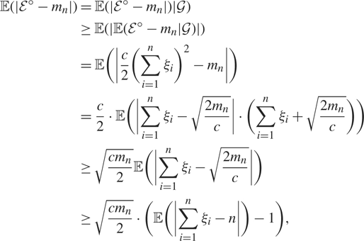
conditionally with respect to 𝒢 (recall Definition 1). Therefore, we have
 $$\mathbb {E}\matrix{
{(|{{\cal E}^ \circ } - {m_n}|)} \hfill & = \hfill & {(|{{\cal E}^ \circ } - {m_n}|)|{\cal G})} \hfill \cr
{} \hfill & \ge \hfill & {(|({{\cal E}^ \circ } - {m_n}|{\cal G})|)} \hfill \cr
{} \hfill & = \hfill & {(|{c \over 2}{{(\sum\limits_{i = 1}^n {\xi _i})}^2} - {m_n}|)} \hfill \cr
{} \hfill & = \hfill & {{c \over 2} \cdot (|\sum\limits_{i = 1}^n {\xi _i} - \sqrt {{{2{m_n}} \over c}} | \cdot (\sum\limits_{i = 1}^n {\xi _i} + \sqrt {{{2{m_n}} \over c}} ))} \hfill \cr
{} \hfill & \ge \hfill & {\sqrt {{{c{m_n}} \over 2}} (|\sum\limits_{i = 1}^n {\xi _i} - \sqrt {{{2{m_n}} \over c}} |)} \hfill \cr
{} \hfill & \ge \hfill & {\sqrt {{{c{m_n}} \over 2}} \cdot ((|\sum\limits_{i = 1}^n {\xi _i} - n|) - 1),} \hfill \cr
} $$
when n is sufficiently large, in particular, when
 $$n - 1 \le \sqrt {2{m_n}/c} = \sqrt {2c{n^2}/2/c} \le n$$
holds. Since
 $$\sum\nolimits_{i = 1}^n {\xi _i}$$
has gamma distribution with parameters nκ and κ, using the formula for the mean absolute deviation of the gamma distribution, we find that
 $$\mathbb {E}(|{{\cal E}^ \circ } - {m_n}|) \ge {{cn} \over 2} \cdot \sqrt {{2 \over \pi }} \cdot \sqrt {n/\kappa } \ge {L_1}{n^{3/2}}$$
holds with appropriate L 1 > 0. Therefore, we have
 $$\mathbb {E}({d_\otimes}({\mathbb {G}_{{\rm{PAG}}}}(n),\mathbb {G}_W^ \circ (n))) \ge {1 \over n} \cdot (|\sum\limits_{1 \le i,j \le n} {U_{ij}} - {V_{ij}}|) = {1 \over {{n^2}}} \cdot (|{{\cal E}^ \circ } - {m_n}|) = \Theta ({n^{ - 1/2}}).$$
On the other hand, since we have
 $$\mathbb {E}(|{{\cal E}^ \circ } - {\cal E}|) = ({c \over 2}\sum\limits_{i = 1}^n \xi _i^2) = {{c(1/\kappa + 1)} \over 2} \cdot n,$$
a similar statement follows for the graph model 𝔾 W (n).
Remark 1. Although it is not the focus of the present paper, we shall say a few words on the influence of the constants c and κ on the bounds. Since the aim was not to produce the sharpest possible expressions for the bounds, the explanations will be somewhat heuristic in nature, and cannot necessarily directly be read off the formulas.
It follows from equation (1) that the larger c is, the larger L 1 in Proposition 3 is, because cmn is an increasing function of c, while the distribution of ξ does not depend on c.Onthe other hand, the proof of the upper bound also produces an expression which is an increasing function of c, if we keep every other parameter fixed (for example, the constant a depends only on κ). This suggests that, although the upper and lower bounds are not the same, the jumble distance in the optimal coupling increases as c is larger. Equation (1) also implies that, at least for the W-random graph model with loops, the lower bound is smaller for larger κ.
The ‘monotonicity’ in c and κ, though of opposing nature, stems from the same phenomenon. In particular, the effect of c might seem surprising at first, since it governs the edge density, and thus one might expect that more edges lead to a better concentration. This is true as n increases due to the degree distribution of the urn model stabilizing and the law of large numbers becoming applicable, but not as c changes, as that shifts this distribution. If either c is increased or κ is decreased, both the graphon W and the degree distribution resulting from the urn model become less ‘flat’, and the variance of the
 $$X_i^*$$
has more of an impact on the resulting W-random graph.
Remark 2. The proof of Proposition 3 shows that even the difference in the number of edges can lead to a positive lower bound on the distance of the two models in the jumble norm. This raises the question of what happens if we modify the models such that the number of edges becomes exactly the same. For example, we consider the random graph
 ${\mathbb {G}}_{\rm{W}}^ \circ (n)$
conditioned on the event that it has ˪cn
2/2˩ edges. However, the coupling of the two models used in the proof of Theorem 1 answers this. The condition means that the sum of the Poisson random variables assigned to the pairs of vertices is equal to ˪cn
2/2˩. As we have seen, this is the same as if we choose the types of ˪cn
2/2˩ edges independently with distribution (ρ
i
), and according to Section 3, we get back the preferential attachment model in this way. Hence the two models have the same distribution under the condition that both have exactly ˪cn
2/2˩ edges.
Remark 3. In this paper we considered the jumble distance between the two random models for the dense PAG
κ
graph, as that is the more natural distance notion for multigraphs generated by unbounded graphons (in this particular case, this corresponds to the unboundedness of the parameters of the Poisson distributions). However, as each finite multigraph generated is bounded per se, one may wonder if it is possible to say anything about the cut distance between 𝔾PAG and
 $${\mathbb {G}}_{\rm{W}}^ \circ $$
, for example.
We recall that the cut distance of two graphs on the same set of n vertices is defined as
 $${d_\otimes}(G,H) = {1 \over {{n^2}}} \cdot \mathop {\max }\limits_{S,T} |\sum\limits_{i \in S,j \in T} {U_{ij}} - {V_{ij}}|.$$
It is easily seen that d □ ≤ d ⊠, hence the upper bounds given for the jumble distance apply a fortiori to the cut distance as well. On the other hand, the methods used in this paper do not yield stronger bounds for the cut-norm distance.
Acknowledgements
The authors are very grateful for the remarks and improvements proposed by the anonymous referee, which ultimately lead to stronger upper and lower bounds.
The first author was supported by the Hungarian National Research, Development and Innovation Office, NKFIH grant K108615 and by the MTA Rényi Institute Lendület ‘Limits of Structures’ Research Group. The second author has received funding from the European Research Council under the European Union’s Seventh Framework Programme (FP7/2007-2013) / ERC grant agreement 617747, the MTA Rényi Institute Lendület ‘Limits of Structures’ Research Group, and was supported by the János Bolyai Research Scholarship of the Hungarian Academy of Sciences.


