2.1. The Model

The model of cointegration is given by the system of equations

where y₁(t) and y₂(t) are continuous time I(1) processes of dimensions m₁ × 1 and m₂ × 1, respectively, B is an m₁ × m₂ matrix of unknown coefficients, and the m₁ × 1 vector u₁(t) and the m₂ × 1 vector u₂(t) are stationary continuous time random disturbances. The initial conditions y₁(0) and y₂(0) are not constrained to be fixed but may be drawn from a certain specified distribution. The long-run equilibrium relations between y₁(t) and y₂(t) are captured by (1), whereas (2) represents the evolution of y₂(t) as a continuous time I(1) process.⁴

Defining the m × 1 vector y(t) ≡ [y₁(t)′, y₂(t)′]′, where m = m₁ + m₂, it is possible to write⁶

where A = [I_m1,−B], J = [I_m1, 0]′ (in which 0 is a null matrix of dimension m₁ × m₂), and

The stationary vector w(t)dt reflects the short-run dynamics of the system that are determined by the properties of u₁ and u₂.

Phillips (1991a) shows that the vector y(t) satisfies the discrete time triangular ECM

and obtains two important results. The first is that the elements of the matrix B are identified directly from the discretely sampled data y(1),y(2),…,y(T), where T denotes sample size. This implies that there is no aliasing problem involved with the identification of cointegrating parameters in cointegrated continuous time systems. The second result is that it is not necessary to derive discrete models that explicitly account for the different ways in which stock and flow variables are observed, at least as far as the estimation of cointegrating parameters is concerned. These findings are in stark contrast to the situation in stationary systems of stochastic differential equations in which aliasing is a concern and in which it is vital to account for the differences between stocks and flows. Phillips derives these results in the cointegrated model by examining the behavior of the spectral density matrix of the observed series at the zero frequency. Certain filtered series, such as flows, do not affect the cointegrating relationships between the variables, because the value of the filter at the zero frequency is unity. This means that the discrete time ECM (4) may be used to estimate the matrix B irrespective of whether the data are stocks, flows, or a mixture of both. It is shown subsequently, however, that although it is possible to estimate the matrix B efficiently for a given data combination of stocks and flows, the way in which the variables are observed does affect the asymptotic variance matrix of the efficient estimators when the different possible data combinations are considered.

2.2. The Sampling Schemes and the Discrete Time Representations

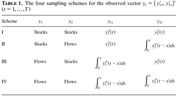
The effects of temporal aggregation are most transparently analyzed by considering, in turn, the four possible combinations⁷

for the flow variables, where in each case t = 1,2,…,T and T denotes sample size. Using y_t to denote the m × 1 vector of observed values, the four sampling schemes of interest are defined in Table 1.

The four sampling schemes for the observed vector yt = [y1t′, y2t′]′ (t = 1,…,T)

Despite the differences arising from the nature of stocks and flows detailed previously, the discrete time ECMs in each of the four stock-flow combinations can nevertheless be written in a common discrete time triangular ECM form, each case differing in the specification of the observable vector y_t (defined previously for each sampling scheme) and in the specification of the unobservable disturbance vector. The precise form of each discrete time ECM is given in Lemma 1, which follows.

LEMMA 1. Let y(t) satisfy the continuous time cointegrated system defined by (1) and (2). Then the observed vector y_t evolves according to the discrete time triangular ECM

in which the components of the disturbance vector ξ_t ≡ [ξ_1t′, ξ_2t′]′ are defined, for each of the four sampling schemes, as follows.

Scheme I.

Scheme II.

Scheme III.

Scheme IV.

The first step in establishing the validity of Lemma 1 is to relate x(t) in (4) directly to u(t), a result that is given in Lemma A1 in Appendix A. Schemes I and IV in Lemma 1, in which y₁ and y₂ are either stocks or flows, are derived directly from (4) and by integrating (4), respectively, the latter case yielding

In the remaining two cases, the joint presence of both stocks and flows requires that the appropriate equations from the systems (4) and (7) are selected and transformed accordingly. Full details of the manipulations are given in the proof of Lemma 1 in Appendix B.

2.3. An Invariance Principle and Asymptotically Efficient Estimation

The derivation of the asymptotic properties of an estimator (efficient or otherwise) of cointegrating parameters is typically based on an invariance principle for ξ_t. Lemma 1 plays an important role in establishing such an invariance principle, because it relates ξ_t to the underlying continuous time disturbance process u(t), about which the following assumptions are made. Let

denote the probability space on which u(t) is defined and let

denote a σ-subfield of

. Then the uniform and strong mixing coefficients, φ_j and α_j, respectively, are defined by

, where

Assumption 1. The continuous time disturbance vector u(t) is a stationary random process with Hermitian positive definite spectral density matrix f (λ) (−∞ < λ < ∞) and satisfies

Assumption 2. The coefficients of the cointegrating matrix B in (1) satisfy |B_ij| < ∞ (i = 1,…,m₁; j = 1,…,m₂).

Assumption 1 specifies u(t) to be a zero mean stationary mixing process in which the mixing coefficients decay sufficiently rapidly to satisfy the stated summability conditions. Furthermore, absolute moments of a sufficiently high order (β) are also required to exist. Mixing conditions are particularly convenient to use in the present context, because in all four sampling schemes ξ_t is a measurable function of u(t) over a finite interval and hence ξ_t inherits the same mixing properties.⁸

LEMMA 2. Under Assumptions 1 and 2, the disturbance vector ξ_t in the discrete time ECM (6) is a stationary random process with Hermitian positive definite spectral density matrix f_ξξ(λ) (−π < λ ≤ π) and satisfies the invariance principle

where the symbol ⇒ denotes weak convergence of the relevant probability measures, [Tr] denotes the integer part of Tr, and S(r) is an m × 1 Brownian motion process on r ∈ [0,1] with covariance matrix Ω = 2πf_ξξ(0).

The invariance principle for ξ_t in Lemma 2 enables the limiting distributions of estimators of B to be expressed in terms of the Brownian motion process S(r). The investigation of efficiency will be carried out with respect to estimators belonging to a well-defined class of estimators. It is convenient to partition S(r) and Ω conformably with y(t) and to define S_1.2(r) = S₁(r) − Ω₁₂Ω₂₂⁻¹S₂(r). Following Saikkonen (1991),

, of the cointegrating matrix B will be defined as one for which

Estimators satisfying the limiting distribution in (8) have alternatively been termed optimal estimators by Phillips (1991b). Because the Brownian motions S_1.2(r) and S₂(r) are independent, the limiting distribution in (8) can also be represented in the now familiar mixed normal form

in which

is the associated probability measure, and the matrix Ω_11.2 = Ω₁₁ − Ω₁₂Ω₂₂⁻¹Ω₂₁ denotes the covariance matrix of S_1.2(r).

The importance of the mixed normal representation of the limiting distribution given in (9) was recognized by Phillips (1989). A number of cointegration estimators are known to have this limiting distribution and, hence, to be asymptotically efficient. Such efficient estimators typically fall into one of two categories. The first type treat the system dynamics either nonparametrically or make nonparametric adjustments to a first-stage estimator. Examples of this type of estimator include the spectral regression estimators suggested by Phillips (1991a), the fully modified estimators of Phillips and Hansen (1990), and the regression estimator of Saikkonen (1991). The second category of estimator is characterized by a fully parametric specification of the system dynamics, typically in vector autoregressive form. Estimators falling within this second category include the maximum likelihood estimators of Johansen (1991) and Phillips (1991b) and the reduced rank estimator of Reinsel (1990).

To compare the asymptotic efficiency of efficient estimators under different combinations of stock and flow data, it is convenient to rewrite the mixed normal distribution in (9) as¹⁰

where

is any unit m₂ × 1 vector, P_γ(γ) is the probability measure associated with γ, and W₂ is an m₂ × 1 vector of standard Brownian motions or Wiener processes (i.e., W₂ is Brownian motion with covariance matrix I_m2). The representation of the distribution in (10) is particularly useful for the purposes of comparison because it is expressed as an integral with respect to the scalar random mixing variate γ that is common to each distribution, regardless of the underlying discrete time sampling scheme. Hence the efficiency comparison focuses on the matrices Ω₂₂ and Ω_11.2, both of which are obtained from Ω, the long-run variance matrix of the process ξ_t. Because the precise form of ξ_t has been shown in Lemma 1 to depend on whether the variables are stocks or flows, it suggests that the relative efficiency of efficient estimators across sampling schemes depends on the nature of the variables themselves. It should be emphasized once more that, for a given sampling scheme, an estimator with the limiting distribution in (8) or (10) is asymptotically efficient. The aim here is to ascertain the extent to which different sampling schemes affect the relative asymptotic efficiency of such estimators across the different sampling schemes. The next section, therefore, derives expressions for Ω₂₂ and Ω_11.2 in each of the four sampling schemes to facilitate such a comparison.

3.1. The Spectral Density Matrix f_ξξ(λ)

The asymptotic variances of efficient estimators have been shown to depend on the submatrices Ω₂₂ and Ω_11.2 that are derived from the long-run variance matrix Ω = 2πf_ξξ(0). Lemma 1 has already provided the relationship between ξ_t and u(t) for each of the four sampling schemes, and this information can be used to derive f_ξξ(λ) from f (λ), the spectral density matrix of u(t). This task is greatly facilitated by the use of filters because ξ_t can be regarded as a filtered version of u(t). The filters corresponding to the time domain representations given in Lemma 1 are provided in Lemma 3.

LEMMA 3. The stationary process ξ_t is related to the continuous time disturbance process u(t) by the filtering equation ξ_t = M(D)u(t), where D denotes the mean square differential operator and the matrix filter function M(z) is defined for each sampling scheme as follows.

Scheme I.

Scheme II.

Scheme III.

Scheme IV.

In the preceding definitions, g(z) = (1 − e^−z)/z and h(z) = e^−z[1 − g(z)]/z.

The filter relating ξ_t and u(t), denoted M(D), is a function of the (mean square) differential operator D because the filter operates on the continuous time process u(t). This does not require, however, that u(t) itself be mean square differentiable, because in none of the sampling schemes does the filter M(D) involve the operation of applying D directly to u(t), so that in no case is Du(t) required to exist. The filter g(D), for example, is the filter associated with the process of integration over the unit interval, so that

. Although this requires that u(t) be integrable in the wide sense

The filter function M(z) is utilized in deriving the spectral density function f_ξξ(λ) of ξ_t. Because ξ_t is a discrete time process and u(t) is a continuous time process, it is necessary to fold back the frequencies in the range (−∞,+∞) into the interval (−π,+π] . The spectral density matrix of ξ_t, regarded as a continuous time process, is given by

where M(iλ)* denotes the transpose of the complex conjugate of M(iλ). This representation follows because iλ is the frequency response function of the operator D and hence M(iλ) is the frequency response function of the filter M(D). The spectral density matrix of the discrete time process ξ_t is then related to f_ξξ^c(λ) by the folding formula:¹²

The properties of the matrix Ω = 2πf_ξξ(0) can be explored from the preceding representation for f_ξξ(λ), and some important and general results are derived in the next section.

3.2. The Asymptotic Variances

The matrix of interest is

, which is obtained from (12) by setting λ = 0. It is convenient, for the presentation of the results, to define the matrix filter function

and also the matrix f_11.2(0) = f₁₁(0) − f₁₂(0) f₂₂(0)⁻¹f₂₁(0), which is obtained from partitions of the spectral matrix f (λ) at the zero frequency in the same way that Ω_11.2 is obtained from Ω. The required expressions for the matrices Ω₂₂ and Ω_11.2 are presented in Theorem 1 for each of Schemes I–IV.

THEOREM 1. The matrices Ω₂₂ and Ω_11.2 appearing in the limiting mixed normal distribution of an efficient estimator of the cointegrating matrix B are given by the following expressions for each of the four sampling schemes.

Scheme I.

Scheme II.

Scheme III.

Scheme IV.

The expressions for the Ω₂₂ and Ω_11.2 matrices given in Theorem 1 are quite general in that they hold for any stationary u(t) process with spectral density matrix f (λ) satisfying Assumption 1. The expressions are convenient representations of these matrices that utilize the precise form of the filter function M(z) in each sampling scheme. Note, however, that the Ω₂₂ matrices are the same in each scheme. This enables the comparisons of estimator efficiency to proceed on the basis of a comparison of the Ω_11.2 matrix in each case. Such a comparison yields the following immediate consequence of Theorem 1.

PROPOSITION 1. The most efficient estimators of cointegrating parameters are obtained when all the variables are flows (Scheme IV).

The validity of this proposition is demonstrated by considering the three matrix differences Ω_11.2^j − Ω_11.2^IV for j = I,II,III and showing that each of these differences is positive semi-definite. This is the sense in which the term efficient is used in Proposition 1, even though the estimators for each sampling scheme are efficient for that particular scheme. Notwithstanding this fact, these results show that, when different sampling schemes are considered, it is flow data that yield the most efficient estimates of cointegrating parameters. If it were possible to choose the way in which one's variables were sampled, then the choice should unambiguously be as flows. Although such a choice is not available to econometricians working with given variables, it does suggest that estimates obtained with flow data are more precise (in the sense of having smaller variances) than those obtained with mixtures of stocks and flows or with stocks alone. Whether it is possible to obtain any improvements at all in the efficiency of estimators based on stock variables is explored in Section 4.

3.3. Continuous Record Asymptotics

It is of interest to compare the efficiency of the estimators based on discretely sampled data with an efficient estimator that is obtained using a continuous record of data. In such circumstances, the classification of variables as stocks or flows is somewhat irrelevant, because the variables are observed on a continuous basis. Although, in practice, continuous time observations are not available to the econometrician, the analysis of the estimator based on a continuous record does serve to illuminate the results obtained earlier.

Assuming that a continuous record of observations is available on y(t) and dy(t) for 0 ≤ t ≤ T, estimation is based on the continuous time triangular system (3). Analogous to the discrete time case, the asymptotic properties of the continuous record estimator

require that, as T → ∞,

where

is an m × 1 Brownian motion process with covariance matrix

denotes the spectral density matrix of w(t). It then follows that the asymptotic distribution of

will have the representation (9) or, equivalently, (10), but in which the matrices Ω₂₂ and Ω_11.2 will be submatrices of

. This is because the spectral matrix of the disturbance process in the model at frequency zero determines the long-run variance matrix and in the continuous record case it is w(t), rather than ξ_t, that constitutes the disturbance vector. These observations lead immediately to the following result.

THEOREM 2. The asymptotic distribution of

is given by

Theorem 2 characterizes the asymptotic distribution of an efficient estimator in the idealized case where observations on the variables are recorded continuously. Note that the matrices

are defined in terms of f (λ), the spectral density matrix of u(t), which enables a direct comparison with the expressions in Theorem 1. Such a comparison yields the following result.

PROPOSITION 2. An efficient estimator obtained using flow data alone (Scheme IV) is asymptotically as efficient as the estimator obtained using a continuous record of data.

This remarkable result indicates that efficient estimators of cointegrating parameters are asymptotically as efficient with discretely sampled flow data as with a continuous record of observations. The observed values of flow variables, by their nature, contain information about the sample path of the variable over each observation interval, whereas stock variables do not contain the same type of information, being observed only at a single point in each interval. Such a difference lies at the heart of the result reported previously.

4.1. The Theory

The result that cointegration estimators are more efficient when obtained using flow data is of little comfort to a researcher working with stock variables. The question arises, therefore, as to whether the results contained in this paper can be used to suggest ways of improving the efficiency of estimators obtained using stock variables. Effectively this reduces to the issue of whether it is possible to approximate the filter function g(z), associated with the operation of integration, which relates the unobservable flow y^F(t) to its discretely observed value,

. Recall that the filter function g(z) appears in the matrix filter function M(z) relating ξ_t to u(t) and that M(2πij) (for integer j) helps to determine the matrix f_ξξ(0), upon which Ω_11.2 is based. The particular values of g(z) that are of interest are, therefore, g(0) = 1 and g(2πij) = 0 for integer j ≠ 0. Given observations on a stock variable at a fixed frequency, there seems little scope for improving efficiency. Attempting to approximate a flow by taking the average of p successive observations using

involves the filter function

. This function satisfies a(0) = 1 and a(2πij) = 1 for integer j ≠ 0, which has no effect whatsoever on asymptotic efficiency.

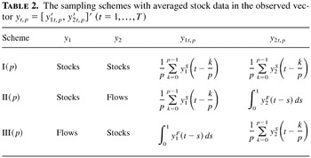
One situation in which efficiency can be improved is where observations on the stock variable are available at a higher frequency than that used for estimation. In models with mixtures of stocks and flows, this situation might arise if it were possible to sample the stocks more frequently than the flows. For example, some stock variables, such as interest rates, exchange rates, and certain prices, are observable at much higher frequencies than flow variables such as consumption, income, and exports. In these cases it would be advantageous to average the stock variables over the (unit) observation interval associated with the sampling of the flows. Suppose that the stock variables are recorded p times each unit observation period. In terms of unit time intervals, the sequence of adjusted stock data is of the form

In terms of filters, the averaged stock variable y_t,p^S is related to y^S(t) by the expression y_t,p^S = σ_p(D)y^S(t), where the filter function σ_p(z) is given by

As p → ∞, the discrete sum determining the averaged variable y_t,p^S converges to an integral, and so

. In practice, although the stock variable y^S(t) may be observed very frequently relative to y_t^F, this limiting case will never be achieved, and so there will always be some loss of efficiency associated with stock variables as compared to flows.

To formalize the arguments, the three cases in which stock variables occur need to be modified to account for the averaging of the stocks over the finer grid of time points comprising each unit time interval. Details of these sampling schemes are given in Table 2, in which y_t,p refers to the m × 1 vector of observations.

The sampling schemes with averaged stock data in the observed vector yt,p = [y1t,p′, y2t,p′]′ (t = 1,…,T)

For the vector y_t,p, the form of the triangular discrete time ECM representation given in (6) is still valid, although the form of the disturbance vector ξ_t is, of course, changed. Lemma 4, which follows, therefore provides the exact discrete time ECM representation when the stock variables are averaged over the unit observation period.

LEMMA 4. Let y(t) satisfy the continuous time cointegrated system defined by (1) and (2). Then the observed vector y_t,p evolves according to the discrete time triangular ECM

in which the components of the disturbance vector ξ_t,p ≡ [ξ_1t,p′, ξ_2t,p′]′ are defined, for each of the three sampling schemes involving averaged stock variables, as follows.

Scheme I(p).

Scheme II(p).

Scheme III(p).

The results in Lemma 4 generalize those in Lemma 1, which may be obtained as a special case of Lemma 4 by setting p = 1. These definitions relate ξ_t,p to the continuous time disturbance process u(t) and, hence, implicitly determine the matrix filter relating these two processes. The precise form of these filters is given in Lemma 5, which is analogous to the results in Lemma 3 for the unadjusted stock variables.

LEMMA 5. The stationary process ξ_t,p is related to the continuous time disturbance process u(t) by the filtering equation ξ_t,p = M_p(D)u(t), where the matrix filter function M_p(z) is defined in each sampling scheme involving averaged stock variables as follows.

Scheme I(p).

Scheme II(p).

Scheme III(p).

The function h_p(z) is defined by h_p(z) = e^−z[σ_p(z) − g(z)]/z.

The dependence of these filter functions on p has been emphasized by the notation M_p(z). In the same way that the filter functions M(z) in Lemma 3 were an essential part of deriving the matrices determining the asymptotic variances of optimal estimators in Section 3, the filter functions in Lemma 5 enable the asymptotic variance matrices to be determined for efficient estimators based on the averaged stock variables. These asymptotic variance matrices are presented in Theorem 3.

THEOREM 3. The matrices Ω₂₂ and Ω_11.2 appearing in the limiting mixed normal distribution of an efficient estimator of the cointegrating matrix B are given by the following expressions under the three sampling schemes involving averaged stock variables.

Scheme I(p).

Scheme II(p).

Scheme III(p).

In each case, note that the only nonzero terms in the expression for Ω_11.2 are multiples of p due to the filter σ_p(z). The expressions in Theorem 3 can be compared directly to those in Theorem 1 to yield the following qualitative result.

PROPOSITION 3. In models containing stock variables, estimators of cointegrating parameters are more efficient when based on the averaged stock variable y_t,p^S than when based on the unadjusted stock variable y_t^S.

The validity of Proposition 3 is established by comparing the Ω_11.2 matrices in Theorems 1 and 3 and showing that the differences are positive definite. The implication for applied work is clear. If it is possible to construct the averaged variables y_t,p^S for stock data, then doing so unambiguously improves the asymptotic efficiency of the cointegration estimators. This could prove to be important in models containing mixed stock and flow variables, because in many cases it will be possible to observe the stock variables at higher frequencies than the flow variables. In such circumstances, the efficiency of the estimators can be improved by applying the filter σ_p(D) to the stock variables.

Some further comments concerning the proposed averaging are in order.¹³

4.2. An Empirical Illustration

It is of interest to ascertain the extent to which the filter σ_p(D) can yield efficiency gains in finite samples, and the long-run money demand relationship provides a convenient model within which to explore such issues empirically. Defining m(t) as the real money stock, y(t) as the level of real income, and r(t) as the interest rate and assuming the variables are individually I(1) processes, the long-run money demand relationship can be cast as the cointegrated system

where the vector u(t) ≡ [u₁(t), u₂(t), u₃(t)]′ is a stationary random disturbance vector. This model is in the form of the cointegrated system (1) and (2), and hence the preceeding results apply to the estimation of the parameters β₁ and β₂.

The data used in this empirical illustration refer to the United States and cover the period January 1, 1959, to December 31, 1999. The money stock series (real M1 money balances) is observed monthly, the interest rate series (Treasury bill rate) is observed daily, and the income series (real GDP) is observed quarterly. The variables m(t) and r(t) are examples of stock variables, whereas y(t) is clearly a flow, although there may, however, be some notion of averaging implicit in the construction of the money stock series. For this reason, quarterly averages of the money stock data were used, although different versions of the interest rate variable were considered. In particular, mid-quarter, end-quarter, and mean-quarter values of the interest rate variable were computed from the daily observations. The preceding theory suggests that the estimates obtained using the latter averages are the most efficient asymptotically, and this empirical application enables the finite sample variances to be compared across the three different sampling schemes for the interest rate.

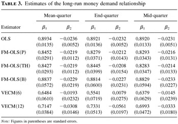
Two types of efficient estimator are considered. The first is the fully modified least squares (FM-OLS) estimator of Phillips and Hansen (1990), based on the triangular ECM representation, and the second is the Gaussian (maximum likelihood) estimator of Reinsel (1990) and Johansen (1991), based on the vector ECM (VECM) representation. The FM-OLS estimators were computed using the automatic bandwidth selection technique of Andrews (1991), based on an AR(1) approximation for the disturbances, to estimate the long-run variance matrix, for three different kernel functions, namely, Parzen, Tukey–Hamming, and Bartlett. These estimators are denoted FM-OLS(P), FM-OLS(TH), and FM-OLS(B) to distinguish the different underlying kernel functions. Using the VECM approach, two estimators were considered. The first uses the Schwartz information criterion to determine the autoregressive order of the system, which turns out to be 6. This estimator is denoted VECM(6). Inspection of the residuals in this system, however, suggests that they are serially correlated, and so the second estimator is based on a system with 12 lags and is denoted VECM(12). Although the second system is less parsimonious in modeling the dynamics, the residuals are closer to being white noise. The estimates of β₁ and β₂ obtained using each estimator are given in Table 3, which also contains the OLS estimates for comparison.

Estimates of the long-run money demand relationship

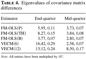
The FM-OLS estimates in Table 3 are remarkably stable across the different treatments of the interest rate data. The estimates using different kernels are also very similar, particularly in the case of the Parzen and Tukey–Hamming kernels. The VECM estimates show more variation both across different treatments of the interest rate data and between different system orders. An interesting feature of the results in Table 3 is that in no case (with the exception of the inefficient OLS estimator) are the standard errors using end-quarter or mid-quarter interest rate data less than those using the mean-quarter data. The theoretical results, however, concern the positive semidefiniteness of the difference in covariance matrices, not a comparison of individual elements of the covariance matrices. With this in mind, we have constructed Table 4, which contains the eigenvalues of the differences in the covariance matrices of the estimators based on unaveraged interest rate data with respect to the averaged data (which the theory suggests should be positive semidefinite).

Eigenvalues of covariance matrix differences

In all cases in Table 4, the relevant covariance matrix differences are positive semidefinite, as predicted by the asymptotic theory. This suggests that averaging stock data can lead to more precise estimates of cointegrating parameters in finite samples. These empirical results are only indicative, however, and should not be interpreted as meaning that such an outcome will always be achieved in finite samples, as the theory derived only relates to the asymptotic distribution of the estimators and not their finite sample distributions.