REPRESENTATION GRAPH

Our basic analytical device is a representation graph (Barthélémy, Martin, and Piggins Reference Barthélémy, Martin and Piggins2014). This is a simple two-dimensional graph, with the number of electors measured on the horizontal axis and the proportion of electoral votes for the Democratic candidate measured on the vertical axis. Currently, the number of electors is 538, one for each of the 100 members of the Senate and 435 members of the House of Representatives, plus three for the District of Columbia.

We used election data to graph how the proportion of electoral votes for the Democrat changes as the size of the House increases or decreases. For example, as House size increases (ceteris paribus), the number of electors will increase, and we move to the right along the horizontal axis in figure 1. For each additional seat in the House, we computed a new congressional apportionment and calculated the resulting proportion of electoral votes for the Democrat.^{Footnote 9} This allowed us to graph the effect of House size on election outcomes. Note that in all of our figures, the Democratic electoral vote percentage is displayed only in increments of five with respect to House size (and total electors), partly concealing what Miller (Reference Miller2014) called the “locally chaotic” relationship between House size and the electoral vote.

Figure 1

2000 Election

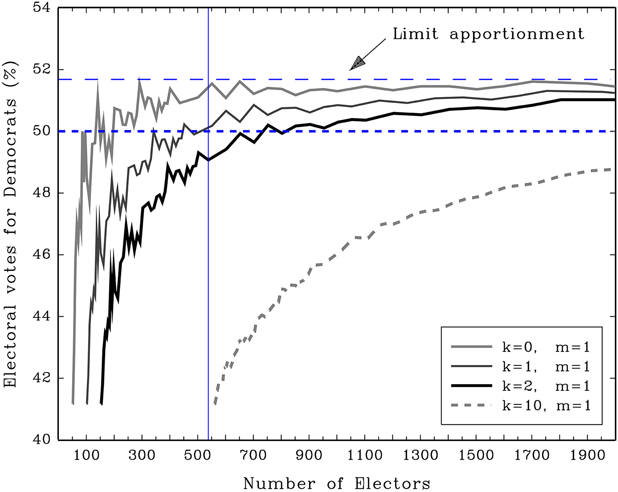
In our figures, if the plotted graph ever crosses 50%, then there is a House size effect.^{Footnote 10} The Electoral College, given that particular House size, will elect a different president. To aid the exposition, we first reproduce figure 1 in Barthélémy, Martin, and Piggins (Reference Barthélémy, Martin and Piggins2014), which refers to the 2000 presidential election.

A vertical line is drawn at 538 electors and a 50% dashed horizontal line is also plotted: k refers to the number of electoral votes each state has by virtue of its Senators and m is the lower bound on the number of electors a state has by virtue of its Representatives. The Constitution specifies that k=2 and m=1, which corresponds to the bold black line in figure 1. Four representation graphs are plotted, one for each of the possible parameter values listed in the legend. The referendum paradox of 2000 can be identified from the figure because the bold black line crosses the vertical line representing 538 electoral votes below the dashed 50% line. But while Gore loses at the existing House size, a sufficiently larger House would have ensured his victory. The representation graph lies above 50% as House size increases. The graph also exhibits the non-monotonicity identified by Neubauer and Zeitlin (Reference Neubauer and Zeitlin2003); the winner oscillates back and forth for a certain interval of House sizes. Neubauer and Zeitlin (Reference Neubauer and Zeitlin2003) showed that if the size of the House is smaller than 491, then Bush is always the winner; if it is greater than 597, then Gore is always the winner (with, somewhat surprisingly, a tie at 655). Between these two numbers, sometimes Bush narrowly wins, sometimes Gore narrowly wins, and sometimes there is a tie. The winner fluctuates chaotically.

However, in figure 1, as House size increases further the graph approaches a second horizontal dashed line labeled “limit apportionment.” This horizontal line is drawn at the electoral vote percentage that the Democratic candidate would obtain if the size of the House was equal to the total apportionment population.^{Footnote 11} In this hypothetical situation, the size of the House is so large that each state, in effect, casts a number of electoral votes equal to its population.^{Footnote 12} As a matter of logic then, under the “winner-takes-all” rule, the limit apportionment electoral vote percentage must equal the percentage of the US apportionment population that resides in states carried by the Democratic candidate. Indeed, in the 2000 election, Gore carried states that accounted for 51.68% of the total apportionment population, which is the limit apportionment electoral vote percentage plotted in figure 1.^{Footnote 13} The corresponding representation graphs for the 1876 election are similar to figure 1.^{Footnote 14}

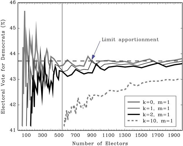
Figure 2 is the corresponding figure for the 2016 presidential election. Importantly, we can see in figure 2 that there is no House size effect. The four representation graphs plotted in figure 2 are safely below 50% on the vertical axis. Unlike 1876 and 2000, a larger House would not have been advantageous to the popular vote winner. Moreover, the limit apportionment is approximately 43.7%.^{Footnote 15}

Figure 2

2016 Election

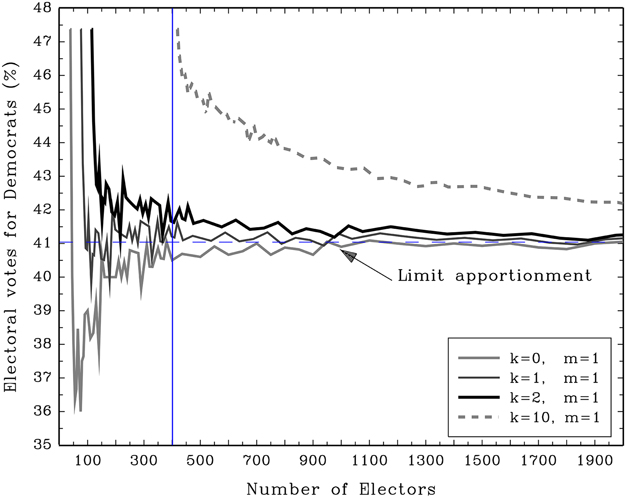
Hillary Clinton’s defeat in the Electoral College is “entrenched” and would have occurred under any of the variations considered. The only historical parallel is the election of 1888, which is shown in figure 4 in Barthélémy, Martin, and Piggins (Reference Barthélémy, Martin and Piggins2014) and reproduced here as figure 3. In 1888, Harrison received 233 electoral votes to Cleveland’s 168; therefore, the vertical line in figure 3 is drawn for a total of 401 electors. The limit apportionment in figure 3 is 41.04%. Like Clinton, a larger House would not have been to Cleveland’s advantage.

Figure 3

1888 Election

An immediate difference between figures 2 and 3 is that the four representation graphs plotted in figure 2 appear to be “inverses” of the corresponding graphs plotted in figure 3. For example, consider the k=10, m=1 graph. In figure 2, this graph begins beneath the limit apportionment electoral percentage and approaches it (from below) as House size increases. In figure 3, the corresponding graph begins above the limit apportionment electoral percentage and approaches it (from above) as House size increases. The fact that a representation graph approaches the limit apportionment electoral vote percentage as House size increases is a mathematical inevitability that was explained previously. However, the difference between the two k=10 graphs requires an explanation.^{Footnote 16} Trump carried 30 states to Clinton’s 21 (including DC); therefore, if the number of electoral votes a state has by virtue of its Senators is increased from 2 to 10, then Trump’s “Senate” electoral votes increase from 60 to 300 and Clinton’s increase from 42 to 210. The smallest size that the Electoral College can be at this point is 561, with each state receiving one “House” electoral vote, with 11 electoral votes allocated to the District of Columbia. This is no different than a federal situation in which a majority of states (including DC) is sufficient to determine the electoral winner without any weight given to their relative populations. In this scenario, Clinton obtains 231/561≅41.18% of the electoral vote, which is why the graph begins below the limit apportionment electoral vote percentage of 43.7%.

As House size increases, the importance of these “Senate” electoral votes declines relative to “House” electoral votes and the graph approaches 43.7%. In 1888, Harrison carried 20 states to Cleveland’s 18, and the states he carried accounted for a majority of the total apportionment population (i.e., approximately 58.96% to Cleveland’s 41.04%).^{Footnote 17} A similar calculation shows that in the k=10, m=1 situation, Cleveland obtains 198/418≅47.37% of the electoral vote, which is why the graph begins above the limit apportionment electoral vote percentage of 41.04%. As before, the graph approaches 41.04% as House size increases. The explanation for the inverses, then, is that Clinton’s loss under federalism was more severe than her loss under a weighted voting system in which each state casts a number of votes equal to its population. For Cleveland, this loss was less severe (recall that he carried slightly less than half of the states).

HOUSE SIZE EFFECT

When is there a House size effect? In an important paper, Miller (Reference Miller2014) identified the following sufficient condition.^{Footnote 18}

As a sufficient condition, a House size effect must arise as a matter of logic if conditions (1) and (2) are jointly satisfied. This sufficient condition was satisfied in both the 1876 and 2000 elections but not in 1888 and 2016. In 2000, Bush carried 30 states to Gore’s 21 (including DC); therefore, condition (1) is satisfied. As noted previously, Gore’s states accounted for approximately 51.68% of the total apportionment population; therefore, condition (2) is satisfied. In 1876, Hayes carried 21 states to Tilden’s 17. However, Tilden’s states accounted for 51.8% of the total apportionment population.^{Footnote 19} Again, conditions (1) and (2) are satisfied.

Therefore, Miller’s sufficient condition shows that a House size effect must be present in both 1876 and 2000. Indeed, we verified through our simulations the existence of a House size effect for the 2000 election in figure 1, and the 1876 election is addressed in figure 5(a) in Barthélémy, Martin, and Piggins (Reference Barthélémy, Martin and Piggins2014).^{Footnote 20}

The intuition behind the Proposition was alluded to previously and we briefly repeat it here. When we are at the constitutional floor of one House seat per state, then the candidate who carries the majority of states (including DC) wins the electoral vote because each state casts three electoral votes (i.e., one “House” vote and two “Senate” votes). In the 2000 election, this candidate was Bush. As House size increases, the importance of these two “Senate” electoral votes decline relative to the “House” electoral votes. As House size increases, further and further, we approach the limit apportionment electoral vote percentage. At this point, the House has grown so large that, in effect, only “House” electoral votes count. The electoral vote percentage (and outcome) is determined by the fraction of the apportionment population in the states carried by the candidates. At some point in this process of making the House larger, the representation graph must cross over the 50% line and (for the 2000 election) Gore is elected President.^{Footnote 21}

Importantly, whereas conditions (1) and (2) are sufficient conditions for a House size effect, they are not necessary conditions. The reason for this is that House seats must be allocated as whole numbers, not fractional numbers. If House seats were allocated fractionally to states, each state could receive its exact “quota” of seats, which is the perfect proportion of the 435 seats in the House of Representatives it is due as a result of its share of the apportionment population. In these circumstances, Miller proved that conditions (1) and (2) are necessary and sufficient for a House size effect.^{Footnote 22}

This scenario would make our simulation in figure 2 unnecessary because the failure of condition (2) to be satisfied would be enough to know that there is no effect present for the 2016 election. However, given that seats are awarded in whole numbers, there is no way of knowing whether a House size effect is present in the 2016 election without running a simulation.

That said, Miller (2014, 266) provided another useful proposition (Proposition A in his paper) that has given historically accurate predictions of a House size effect, despite not being quite valid as a theoretical proposition (again, because House seats must be allocated as whole numbers). Proposition A states that a presidential election is subject to the House size effect if and only if: (1) one candidate (say A) wins a majority of the Senate electoral votes, and (2) the other candidate (say B) wins a majority of the House electoral votes. As discussed previously, Trump carried 30 states and therefore won 60 “Senate” electoral votes (a majority). However, he also won 305–60=245 “House” electoral votes (again, a majority). Therefore, condition (2) does not hold and Proposition A predicts that there will be no House size effect. Our simulation shows that this prediction is accurate.

In summary, figure 2 shows that Trump’s election in 2016—like Harrison’s in 1888 but unlike Hayes’s in 1876 and Bush’s in 2000—entailed an entrenched referendum paradox. It is tempting to think that one way to avoid the referendum paradox is to abandon “winner-takes-all” and allow states to allocate their electoral votes fractionally, in proportion to the popular vote percentages in each state.^{Footnote 23} However, such proportionality in general does not overcome the referendum paradox because it remains true that state electoral votes are not precisely proportional to state populations (and still less to state presidential popular votes). For example, in the 2000 election, such a procedure would generate approximately 259.17 electoral votes for Bush compared with 258.27 for Gore.^{Footnote 24} As this example demonstrates, the presence of third-party candidates means that a majority winner in the Electoral College is unlikely under a fractional system.^{Footnote 25} In the 2016 election, fractional voting would have produced approximately 255.43 electoral votes for Clinton compared with 249.07 for Trump. Unlike the election in 2000, Clinton (the popular vote winner) would emerge as the plurality winner in this case.