




No CrossRef data available.
THE DICKEY–FULLER TEST FOR EXPONENTIAL RANDOM WALKS
Published online by Cambridge University Press: 04 August 2003
Abstract
A common test in econometrics is the Dickey–Fuller test, which is based on the test statistic  . We investigate the behavior of the test statistic if the data yt are given by an exponential random walk exp(Zt) where Zt = Zt−1 + σεt and the εt are independent and identically distributed random variables. The test statistic DF(T) is a nonlinear transformation of the partial sums of εt process. Under certain moment conditions on the εt we show that
 tends to one as λ → 0. For the particular case that the εt define a simple random walk it is shown that plimT→∞ DF(T)/T exists and the limit is evaluated. The theoretical results are illustrated by some simulation experiments.We gratefully acknowledge the help of an anonymous referee whose comments on the first two versions of this paper enabled us to reduce the number of mistakes and to increase the clarity of presentation. The authors' research was supported in part by Sonderforschungsbereich 475, University of Dortmund.
Information
- Type
- Research Article
- Information
- Copyright
- © 2003 Cambridge University Press
1. INTRODUCTION
A common test in econometrics is the Dickey–Fuller test, which for data yt, t = 0,…,T is defined by the test statistic

The purpose of the test is to investigate the adequacy of a random walk model for the data yt. In this paper we investigate the behavior of the test statistic if the data are better described by an exponential random walk. To be precise we consider a stochastic process Yt,t = 0,…,T given by

where

and the εt are independent and identically distributed (i.i.d.) random variables. We write the test statistic in the form

where

This is a nonlinear transformation of the partial sums of εt process. Park and Phillips (1998) have developed a general method of treating nonlinear functionals of integrated time series, but unfortunately their results do not cover the asymptotic behavior of (2). There are two reasons for this. First, if we write the statistic in the form

it is seen that the functional does not fit into the Park and Phillips framework because of the explicit appearance of the increment εt. The second reason is not quite so obvious. Park and Phillips develop a theory that is applicable to the the sum S0(T) of (3). Suppose that the εt have mean zero and finite nonzero variance. On writing

Theorem 5.5 of Park and Phillips (1998) gives

where ⇒ denotes weak convergence, L(x,t) is the local time of Brownian motion W on [0,1], and

The interpretation of L(x,t) as an occupation time density and the continuity of L(x,t) make it clear that L(1,smax) = 0. The consequence is that (5) reduces to

so that it is of no help in analyzing the Dickey–Fuller statistic. For this we require the exact order of magnitude of S0(T). This is derived in the next section. In Section 3 we apply the result to the Dickey–Fuller statistic, which allows us to derive the correct order of magnitude of the statistic. In the particular case of the simple random walk the exact limiting behavior can be given. This is done in Section 4. Finally in Section 5 we give the results of some simulations.
2. THE ASYMPTOTIC BEHAVIOR OF [sum ]0T exp(σZt)
We prove the following theorem.
THEOREM 1. Suppose the increments (εi)1∞ are i.i.d. and satisfy

Then for all γ > 0

Proof. Clearly

so it is sufficient to prove

which is equivalent to

which in turn follows from

for some constant A. Consider the term

where Ft,T denotes the distribution function of MT − Zt. In the following discussion we make repeated use of the reversal procedure described on page 394 of Feller (1971). We have

where

. The proof of Theorem 1 relies entirely on the estimate

where now and in the discussion that follows a and b denote generic constants whose values may change at each appearance. As

converges weakly to the maximum of a Brownian motion on [0,1], (12) would follow immediately if a Berry–Esséen type result were available for the distribution of

. We have not found such a result in the literature so we now give a proof that relies on properties of the random walk in

as given in Chapter XII of Feller (1971). For the sake of simplicity we assume that the random variables Zt have a continuous distribution function, in which case the distinction between weak and strict variables is unnecessary (see Feller, 1971, pp. 392–393). We consider the case of strict variables only; the arguments for weak variables are to be found in Chapter 12 of Feller (1971). We have

where


To estimate qj in (15) we note that the assumptions of the theorem imply

for some finite constant c (see Feller, 1971, p. 612). From this we deduce

(see Feller, 1971, pp. 418–419).
We turn to estimates for Hj(x) of (14). We note first that

As Zn − Zn/2 is independent of Zn/2 the Berry–Esséen theorem for

gives

and on substituting this into (18) we obtain

where we have used the argument leading to (17). The second estimate for Hn(x) that we require is

where ψ(x) is the renewal function of the first ladder height (see the duality lemma in Feller, 1971, p. 395). The inequality in (20) follows from the renewal theorem (Feller, 1971, pp. 358–366).
Applying the inequalities (17), (19), and (20) in (13) we obtain

where the first estimate follows from (17) and (20) and the second from (17) and (19). This finally proves (12), and on using this in (11) we obtain

From (21) we conclude

This proves (9) with A = a and with it the theorem. █
3. THE ASYMPTOTIC BEHAVIOR OF THE DICKEY–FULLER STATISTIC
We turn to the asymptotic behavior of the Dickey–Fuller statistic when applied to the Yt.
THEOREM 2. Suppose the increments (εi)1∞ are i.i.d. and satisfy

Then

Proof. The lower bound of −T follows directly from (2) on noting that

is always positive. To obtain the upper bound we require an upper bound for the sum S1(T). This requires an analysis of the path (t,Zt)0T with Z0 = 0. We denote the path by B(T) and write S1(B(T)) = S1(T). If part of the path is constant, that is, Zt = Zt+1 = ··· = Zt+s for some s ≥ 1, then the points (t + 1,Zt+1),…,(t + s,Zt+s) can be removed without changing the value of S1. Without loss of generality we can therefore suppose that the path has no intervals where it is constant. We consider the effect of removing the local maxima from the path B(T). As the path contains no intervals of constancy there is a local maximum at the point t if

We suppose that Zt−1 ≤ Zt+1 < Zt. A similar argument works if Zt+1 ≤ Zt−1 < Zt. A new path of length T − 1 is constructed by setting

. We denote this new path by

and set Δ = Zt − Zt+1 and γ + Δ = Zt − Zt−1 with γ and Δ both nonnegative. We have

We note that the value of the final point of the path is not altered, i.e.,

. Under the conditions of the theorem

for all a > 0 so that the global maximum is an interior local maximum with probability tending to one as T tends to infinity. We reserve the Δ in (23) for the point corresponding to the global maximum. We now proceed to remove all local maxima and finally obtain a path

of length T − k with no local maxima and that satisfies

As

has no local maxima it follows that the global maximum of this path is located either at 0 or T − k. As the removal of local maxima does not alter the value of the last point we have

, and hence

As

for any sequence aT with

it follows that

, which yields

This combined with the result of Theorem 1 implies

To complete the proof of the theorem it suffices to show that

where Δ* = min{εt, − εt+1} on MT = Zt. Conditioning on MT = Zt we have for εt

and

As the εj are assumed to be independently distributed the inequalities (27) have no effect on the conditional distribution of εt. The inequalities (26) may be written in the form

On conditioning on ε1,…,εt−1 and using the fact that

for any random variable X and for any x and a ≥ 0 we deduce

Similarly we have

These latter inequalities imply

from which we may deduce (25). This completes the proof of the theorem. █
4. THE SIMPLE RANDOM WALK
In the case of the simple random walk a more precise result is possible. In fact we state the theorem somewhat more generally as we need only the properties (28) and (29), which follows and they are satisfied for the simple random walk. In particular we do not require that the εi are independently or identically distributed.
THEOREM 3. Suppose that the process Zt satisfies

and

for all a > 0. Then

where σ is as in (1).
Proof. Without loss of generality we may set Z0 = 0, and to ease the notation we consider only the case σ = 1. Given a level j we consider those times t, if any, for which Zt = j and Zt+1 = j + 1. These are the set of up-crossings from j to j + 1. Similarly we define the set of down-crossings from j + 1 to j as those points t, if any, for which Zt = j + 1 and Zt+1 = j. Consider first a path with ZT ≥ 1. Then for all j ≥ ZT and for all j ≤ −1 the number of up-crossings from j to j + 1 is equal to the number of down-crossings from j + 1 to j. For 0 ≤ j ≤ ZT − 1 the number of up-crossings from j to j + 1 exceeds the number of down-crossings from j + 1 to j by 1. Similarly if ZT ≤ 0 then for j ≥ 0 and j ≤ ZT − 1 the number of up-crossings from j to j + 1 is equal to the number of down-crossings from j + 1 to j. For ZT ≤ j ≤ −1 the number of down-crossings from j + 1 to j exceeds the number of up-crossings from j to j + 1 by 1. For each level j let N(j,T) denote the number of up-crossings from j to j + 1 that can be paired with a down-crossing from j + 1 to j. Further let E(j,T) denote the excess of up-crossings from j to j + 1 over the down-crossings from j + 1 to j. The preceding argument shows that E(j,T) is either −1, 0, or 1.
The contribution of an up-crossing from j to j + 1 to the sum S1(T) of (3) is

Similarly the contribution to S1(T) of a down-crossing from j + 1 to j is

We may therefore write

Similarly for the sum S0(T) we have

Suppose now that ZT > 0. Then the argument given previously shows that E(j,T) = 0 for j ≥ ZT and consequently

Similarly if ZT ≤ 0 then

On combining these last two inequalities we obtain

Consider a random walk satisfying

It follows from the arguments given previously that N(j,T) ≥ 1 for j = MT − 1. This implies

by (33) and consequently

From (29) it follows that there exists a sequence (aT)1∞ satisfying limT→∞ aT = ∞ such that

Using this in (34) gives

from which we obtain with (31)

and with (32)

On using these asymptotic equivalences in (3) we have

which proves the theorem. █
5. SIMULATIONS
Figure 1 shows the results of a simulation of a simple random walk with the εi i.i.d. and taking the values 1 and −1 with probability 0.5, σ = 0.01, and T = 100,000. Part (a) shows the path behavior of the Zt-process, (b) shows the corresponding process Yt, and (c) shows the path behavior of the Dickey–Fuller statistic. The final value of the statistic is −5.163337e − 05, which compares well with the theoretical slope given by


(a) The zt process for the simple random walk with σ = 0.01 and T = 100,000. (b) The corresponding yt process. (c) The path behavior of the Dickey–Fuller statistic.
Figure 2 shows the corresponding results when the εi are i.i.d. standard Gaussian random variables. The variability of the individual paths is very high. To overcome this 500 paths of length 20,000 were simulated with σ = 0.01 and the εi being standard Gaussian white noise. The mean value of the Dickey–Fuller statistic was calculated at each of the time points 1,000, (1,000), 20,000. The results are shown in Figure 3, where a linear trend is apparent. This is consistent with the main theorem. It makes plausible the conjecture that the probability limit plimT→∞ DF(T)/T exists and is negative and finite also in the Gaussian case


(a) The zt process for standard Gaussian increments with σ = 0.01 and T = 100,000. (b) The corresponding yt process. (c) The path behavior of the Dickey–Fuller statistic.

The value of the Dickey–Fuller statistic averaged over 500 simulated paths.
with d > 0 and finite. We offer no proof of this. There well may be other distributions for which (36) holds true, and in this case one can expect the constant d to be dependent on the underlying distribution of the εi.
References
REFERENCES
Feller, W.
(1971)
An Introduction to Probability Theory and Its Applications,
2nd ed.,
vol. 2.
New York:
Wiley.
Park, J.Y. &
Phillips, P.C.B.
(1998)
Asymptotics for nonlinear transformations of integrated time series.
Econometric Theory
15,
269–298.Google Scholar
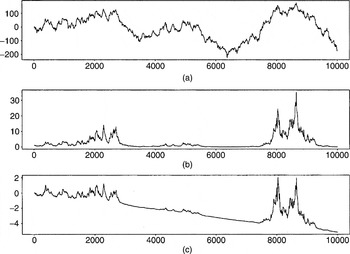
(a) The zt process for the simple random walk with σ = 0.01 and T = 100,000. (b) The corresponding yt process. (c) The path behavior of the Dickey–Fuller statistic.
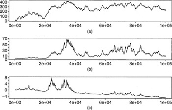
(a) The zt process for standard Gaussian increments with σ = 0.01 and T = 100,000. (b) The corresponding yt process. (c) The path behavior of the Dickey–Fuller statistic.
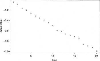
The value of the Dickey–Fuller statistic averaged over 500 simulated paths.
 You have
Access
- 3
- Cited by