2.1 Data

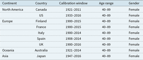
We consider mortality data from the female populations of nine countries which span four continents. All of the required data are obtained from the Human Mortality Database. The age range we use is 40–89 years, which covers typical ages of annuitants/pensioners and excludes the extreme ages for which the data are extrapolated values instead of raw counts. To better satisfy the data requirements of GARCH-type model and discern the potential asymmetry in mortality volatility, we use all available data (over the chosen age range) from 1900Footnote ¹. A summary of the mortality data used is summarised in Table 1.

Table 1.

A summary of the mortality data used in this paper.

2.2 The Lee–Carter structure

Following Zhou & Li (Reference Zhou and Li2019a), we assume that mortality follows the Lee–Carter structure:

(1) \begin{equation}\ln m_{x,t} = a_x + b_x \kappa_t\end{equation}

where $m_{x,t}$ is the central death rate at age x and in year t, $a_x$ is an age-specific parameter measuring the average level of mortality at age x, $\kappa_t$ is the time-varying index (also known as the period effect) capturing the overall level of mortality in year t and $b_x$ is an age-specific parameter reflecting the sensitivity of $m_{x,t}$ to changes in $\kappa_t$ .

The dynamics of $\kappa_t$ is specified as

(2) \begin{align}\kappa_t &= \kappa_{t-1} + \mu + \epsilon_t\end{align}

where $\mu$ is the drift term representing the expected rate of change in $\kappa_t$ , and $\epsilon_t$ is the time-t innovation which has a zero meanFootnote ². While most previous studies in stochastic mortality modelling assume that the variance of $\epsilon_t$ is time-invariant, we permit the (conditional) variance of $\epsilon_t$ to vary over timeFootnote ³. We use $\sigma_t^2$ to represent the conditional variance of $\epsilon_t$ .

In the rest of this section, we first identify any possible conditional heteroskedasticity, that is, the phenomenon that $\sigma_t^2$ is time-varying, for each of the nine populations. We then move to our first research objective to investigate the possibility that $\sigma_t^2$ responds asymmetrically to positive and negative shocks (innovations) prior to time t.

2.3 Conditional heteroskedasticity

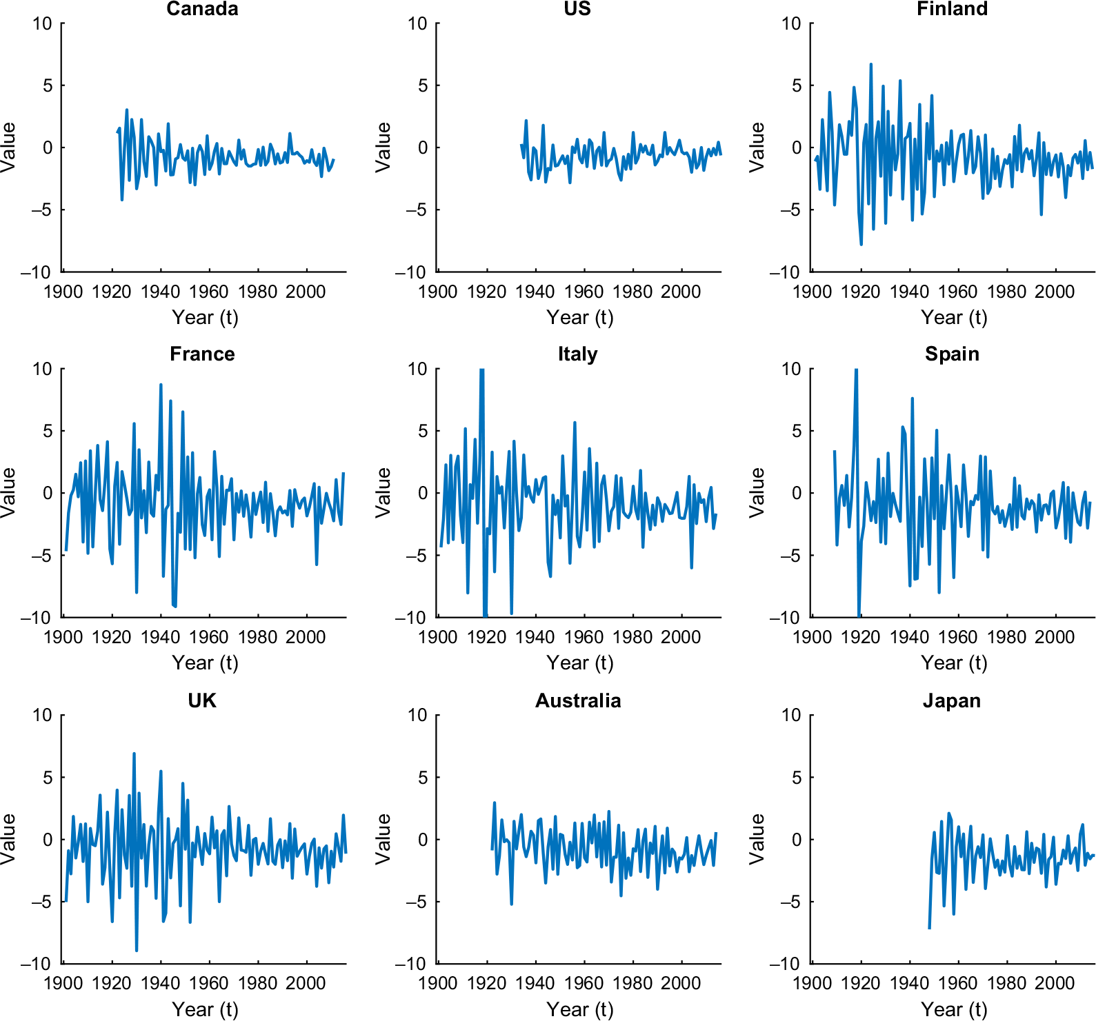
Using the Poisson maximum likelihood method (Brouhns et al., Reference Brouhns, Denuit and Vermunt2002), we obtain estimates of parameters in equation (1). Figure 1 shows the estimated series of $(\kappa_t - \kappa_{t -1})$ for each of the nine populations under consideration. For all populations except Australia and the US, the variation in $(\kappa_t - \kappa_{t -1})$ clearly varies over time. In particular, the variation seems more pronounced during certain periods, such as 1910s and 1930s. Such a pattern suggests that conditional heteroskedasticity exists.

Figure 1

The estimated series of $(\kappa_t - \kappa_{t -1})$ for each of the nine populations under consideration.

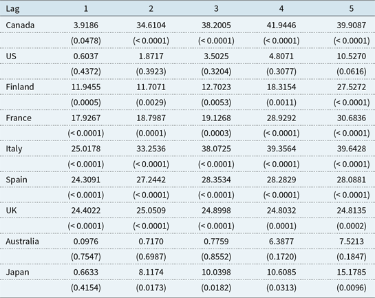
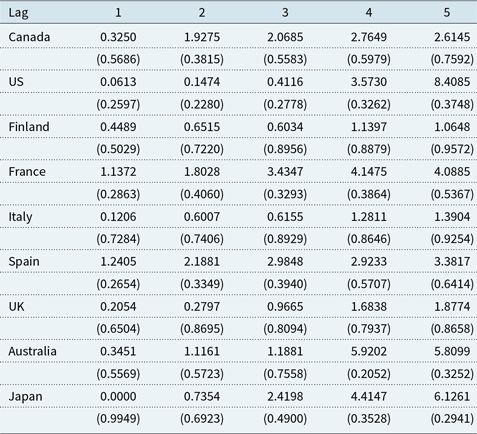
To verify the existence of conditional heteroskedasticity, we apply Engle’s ARCH test to the series of $(\kappa_t - \kappa_{t - 1})^2$ for each population. The test results are reported in Table 2. Except for US and Australia, the test results suggest a rejection of the null hypothesis that $(\kappa_t - \kappa_{t - 1})^2$ possesses no serial correlation, confirming the existence of conditional heteroskedasticity. We also apply the Ljung–Box test to the series of $(\kappa_t - \kappa_{t - 1})^2$ for each population. The test results (not shown for the sake of space) point to the same conclusion.

Table 2.

The test statistic and the p-value (in parentheses) of the Engle’s ARCH test (at lag 1 to 5) applied to the series of $(\kappa_t - \kappa_{t-1})$ for the each of the nine populations under consideration.

In our preliminary modelling work, we estimate a GARCH(1,1) model to the series of $\epsilon_t$ (i.e., the mean corrected series of $(\kappa_t - \kappa_{t-1})$ ) for each of the nine populations under consideration. The GARCH(1,1) model can be expressed as

(3) \begin{align}\hspace*{-1pt}\epsilon_t &= \sigma_t \eta_t \hspace*{58pt}\end{align}

(4) \begin{align}\sigma^2_t &= \omega + \alpha \epsilon_{t-1}^2 + \beta \sigma^2_{t-1}\end{align}

where $\sigma^2_t$ is the conditional variance of $\epsilon_t$ , $\eta_t$ -s are independent and identically distributed (i.i.d.) standard normal random variables, and $\omega$ , $\alpha$ and $\beta$ are constant parameters. In particular, parameters $\alpha$ and $\beta$ govern the dependence of the time-t conditional variance on the time- $(t-1)$ squared innovation and the time- $(t-1)$ conditional variance, respectively.

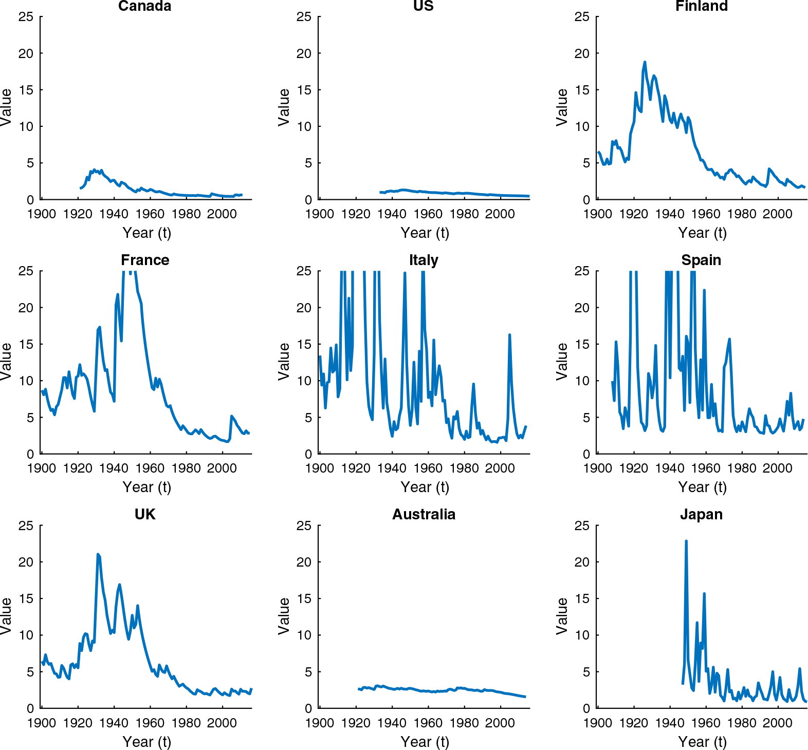
Having fitted the GARCH(1,1) model, the inferred values of $\sigma^2_t$ over the calibration window are extracted and are reported in Figure 2. The existence of conditional heteroskedasticity is further supported by the fact that the patterns of the inferred values of $\sigma^2_t$ over the calibration window are far from being flat for all of the populations considered, except US and Australia. We then apply Engle’s ARCH test to the series of squared standardised residualsFootnote ⁴ for each population. Reported in Table 3, the test results indicate no significant serial correlations in the squared standardised residuals, suggesting that conditional heteroskedasticity is adequately captured by the GARCH(1,1) models. We also apply the Ljung–Box test to the series of squared standardised residuals for each population. The test results (not shown for the sake of space) point to the same conclusion.

Figure 2

The inferred values of $\sigma^2_t$ derived from the estimated GARCH(1,1) models for the nine populations under consideration.

Table 3.

The test statistic and p-value (in parentheses) of the Engle’s ARCH test (at lag 1 to 5) applied to the squared standardised residuals from the GARCH(1,1) for each of the nine populations under consideration.

While the GARCH(1,1) model appears to have captured conditional heteroskedasticity adequately, it does not capture any asymmetry in volatility. It is clear from equation (4) that a positive shock (innovation) at time $t-1$ , say $|\epsilon^*_{t-1}|$ , and a negative shock of the same magnitude, that is, $-|\epsilon^*_{t-1}|$ , have exactly the same impact on the time-t conditional variance.

2.4 Asymmetry in mortality volatility

To investigate the potential asymmetry in mortality volatility, a wider range of GARCH-type models are considered. The additional models include the E-GARCH model, the GJR-GARCH model, the N-GARCH model and the T-GARCH model. These models differ from the GARCH model in the way in which the dynamics of the conditional variance $\sigma_t^2$ is specified. We consider an order of (1,1) for all of the additional models, because the results in the previous subsection suggest that this order can adequately capture the serial correlation in the conditional variances.

Below we describe, for each of the additional GARCH-type models, the specification of the dynamics of $\sigma^2_t$ and the way in which the asymmetry in volatility is captured. In all of the models, $\omega$ , $\alpha$ , $\beta$ and $\gamma$ are constant parameters, and $\gamma$ is the parameter controlling the asymmetry in volatility.

• E-GARCH

  The E-GARCH(1,1) model assumes that

  (5) \begin{equation} \ln(\sigma^2_{t}) = \omega + \gamma \eta_{t-1} + \alpha \left( |\eta_{t-1}| - \sqrt{\frac{2}{\pi}} \right) + \beta \ln \sigma^2_{t-1} \end{equation}
  where $\eta_{t-1} = \epsilon_{t-1}/\sigma_{t-1}$ . A positive time- $(t-1)$ innovation with a magnitude of $|\epsilon^*_{t-1}|$ affects $\ln(\sigma_t^2)$ by $\gamma |\epsilon^*_{t-1}|/\sigma_{t-1} + \alpha ( |\epsilon^*_{t-1}|/\sigma_{t-1} - \sqrt{2/\pi} )$ , whereas an otherwise identical negative innovation affects $\ln(\sigma_t^2)$ by $-\gamma |\epsilon^*_{t-1}|/\sigma_{t-1} + \alpha ( |\epsilon^*_{t-1}|/\sigma_{t-1} - \sqrt{2/\pi} )$ .

• GJR-GARCH

  The GJR-GARCH(1,1) model assumes that

  (6) \begin{equation}\sigma^2_{t} = \omega + \alpha \epsilon^2_{t-1} + \gamma \epsilon^2_{t-1} \mathcal{I}_{\{\epsilon_{t-1}<0\}} + \beta \sigma^2_{t-1} \end{equation}
  where $\mathcal{I}_{A}$ is an indicator function which equals 1 if event A holds true and 0 otherwise. A positive time- $(t-1)$ innovation with a magnitude of $|\epsilon^*_{t-1}|$ affects $\sigma_t^2$ by $\alpha (\epsilon^*_{t-1})^2$ , whereas an otherwise identical negative innovation affects $\sigma_t^2$ by $(\alpha + \gamma)(\epsilon^*_{t-1})^2$ .

• N-GARCH

  The N-GARCH(1,1) model assumes that

  (7) \begin{equation} \sigma^2_{t} = \omega + \alpha\sigma^2_{t-1}(\eta_{t-1}-\gamma)^2 + \beta\sigma^2_{t-1} \end{equation}
  A positive time- $(t-1)$ innovation with a magnitude of $|\epsilon^*_{t-1}|$ affects $\sigma_t^2$ by $\alpha\sigma^2_{t-1}(|\epsilon^*_{t-1}|/\sigma_{t-1}-\gamma)^2$ , whereas an otherwise identical negative innovation affects $\sigma_t^2$ by $\alpha\sigma^2_{t-1}(-|\epsilon^*_{t-1}|/\sigma_{t-1}-\gamma)^2$ .

• T-GARCH

  The T-GARCH(1,1) model assumes that

  (8) \begin{equation} \sigma_{t} = \omega + \alpha (|\epsilon_{t-1}| - \gamma\epsilon_{t-1}) + \beta \sigma_{t-1} \end{equation}
  A positive time- $(t-1)$ innovation with a magnitude of $|\epsilon^*_{t-1}|$ affects $\sigma_t$ by $\alpha(1 - \gamma) |\epsilon^*_{t-1}|$ , whereas an otherwise identical negative innovation affects $\sigma_t$ by $\alpha(1 + \gamma) |\epsilon^*_{t-1}|$ .

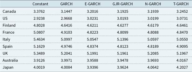
We apply the above-mentioned models to all of the nine populations under consideration. To compare the performances of these models as well as the GARCH model and the constant volatility assumption, we consider the Bayesian information criterion (BIC), which is defined such that a lower BIC value indicates a better goodness-of-fit with the number of model parameters being taken into account. The results are reported in Table 4.

Table 4.

The BIC values resulting from the constant volatility assumption, the GARCH model and four GARCH-type models that incorporate asymmetry in volatility, fitted to the mean-corrected series of $(\kappa_t - \kappa_{t-1})$ for the nine populations under consideration.

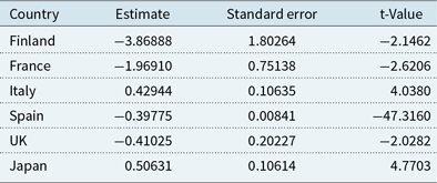
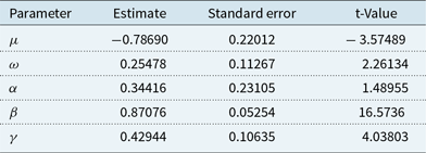
In line with the results in section 2.3, the constant volatility assumption produces the lowest BIC values for US and Australia. For all but one of the remaining populations, the best performing model is either the E-GARCH, GJR-GARCH or T-GARCH model, suggesting that there exists asymmetry in mortality volatility. We further examine the estimates of parameter $\gamma$ for these populations (Table 5). It is found that all of the six estimates of $\gamma$ are significant at any reasonable level of significance, further confirming the existence of asymmetry in mortality volatility and the need for capturing it. In addition to the BIC, the Akaike information criterion and the Hannan–Quinn information criterion are considered. These two criteria also suggest the existence of asymmetry in mortality volatility for most of the populations considered.

Table 5.

Estimates (and their standard errors and t-values) of parameter $\gamma$ in the best performing models for Finland, France, Italy, Spain, UK and Japan.

The meaning of the sign of parameter $\gamma$ depends on how the asymmetric GARCH model is constructed. For the E-GARCH model, a positive $\gamma$ means that the impact of a positive shock on volatility is more prominent than a negative shock, whereas for the GJR-GARCH, N-GARCH and T-GARCH models, the opposite is true. The estimates of $\gamma$ reported in Table 5 thus suggest that mortality volatility is more responsive to positive shocks than negative shocks. This property is conceivable, because in the context of mortality modelling, positive shocks that are due to events such as wars and pandemics typically have a more significant and immediate impact compared to negative shocks that arise from medical breakthroughs.

3.1 The key building block

Denote by $q_{x,t}$ the probability that an individual who has survived to age x at time $t-1$ dies between time $t-1$ and t. We have

\[S_{x,t}(T) = \prod_{s=1}^{T}(1-q_{x+s-1,t+s}) \]

being the ex post probability that an individual who has survived to age x at time t would have survived to time $t+T$ for $T=1,2,\ldots$ . Assuming a constant force of mortality between consecutive integer ages, which in turn implies that $q_{x,t} = 1-\exp(-m_{x,t})$ , we can express $S_{x,t}(T)$ as follows:

(9) \begin{align}S_{x,t}(T) &= \prod_{s=1}^{T}\exp(-m_{x+s-1,t+s}) \nonumber \\ &= \exp\left(-\sum_{s=1}^{T}\exp(a_{x+s-1}+b_{x+s-1}\kappa_{t+s})\right)\\[3pt] & = \exp\left(-\sum_{s=1}^{T}\exp(Y_{x,t}(s))\right)\nonumber\end{align}

(10) \begin{align} = \exp(-W_{x,t}(T))\hspace*{65pt}\end{align}

where

(11) \begin{equation}Y_{x,t}(s)=a_{x+s-1}+b_{x+s-1}\kappa_{t+s}\end{equation}

and

(12) \begin{equation}W_{x,t}(T)=\sum_{s=1}^{T}\exp(Y_{x,t}(s))\end{equation}

are defined to make the expressions of longevity Greeks more compact.

We set time 0 to the end point of the calibration window to which the model is fitted. Using equations (2) and (3), we obtain

(13) \begin{equation}\kappa_{t} = \kappa_0 + t\mu + \sum_{s=1}^{t}\sigma_{s}\eta_{s}, \quad t \geq 1\end{equation}

so that

(14) \begin{align}S_{x,t}(T) = \exp\left(-\sum_{s=1}^{T}\exp\left(a_{x+s-1}+b_{x+s-1}\left(\kappa_0 + (t+s)\mu + \sum_{u=1}^{t+s}\sigma_{u}\eta_{u}\right)\right)\right)\end{align}

Zhou & Li (Reference Zhou and Li2019a) assume a GARCH(1,1) model, which implies that

(15) \begin{align}\sigma^2_s = \begin{cases}\omega \left(1+\sum_{u=1}^{s-1} \prod_{v=1}^{u} (\alpha \eta^2_{s-v} + \beta)\right) + (\alpha \epsilon_{0}^2 + \beta \sigma^2_{0}) \prod_{v=1}^{s-1} (\alpha \eta^2_{s-v} + \beta) & \quad \text{if } s \geq 2 \\[8pt] \omega + \alpha \epsilon_{0}^2 + \beta \sigma^2_{0} & \quad \text{if } s=1\\\end{cases}\end{align}

Let $\mathcal{F}_t$ be the information about the evolution of mortality up to and including time t. It follows from equations (14) and (15) that given $\mathcal{F}_0$ , $S_{x,t}(T)$ depends on $\kappa_0$ (the time-0 value of the period effect), $\sigma^2_0$ (the time-0 value of the conditional volatility) and a sequence of i.i.d. standard normal random variables $\{\eta_s;\, s = 1,\ldots,t+T \}$ . It is clear that $S_{x,t}(T)$ given $\mathcal{F}_0$ is a random variable due to its dependence on $\{\eta_s;\, s = 1,\ldots,t+T \}$ .

Finally, we arrive at the following key building block of the longevity Greeks framework of Zhou & Li (Reference Zhou and Li2019a):

\[p_{x,t}(T,\kappa_0,\sigma^2_0) \coloneqq \mathrm{E}[{S_{x,t}(T)|\mathcal{F}_0}]\]

which can be interpreted to mean the probability for an individual aged x at time t to survive to time $t + T$ , given the information about the evolution of mortality up to and including time 0.

3.2 Longevity Greeks for $p_{x,t}(T,\kappa_0,\sigma^2_0)$

The longevity Greeks for $p_{x,t}(T,\kappa_0,\sigma^2_0)$ are obtained by taking the partial derivatives of $p_{x,t}(T,\kappa_0,\sigma^2_0)$ with respect to either $\kappa_0$ or $\sigma^2_0$ .

The longevity delta for $p_{x,t}(T,\kappa_0,\sigma^2_0)$ is

\[\frac{\partial p_{x,t}(T,\kappa_0,\sigma^2_0)}{\partial \kappa_0} = -\sum_{s=1}^T b_{x+s-1} \mathrm{E}[{\exp(Y_{x,t}(s)-W_{x,t}(T)) | \mathcal{F}_0}]\]

a quantity which measures the first-order sensitivity of $p_{x,t}(T,\kappa_0,\sigma^2_0)$ to changes in $\kappa_0$ .

The longevity gamma for $p_{x,t}(T,\kappa_0,\sigma^2_0)$ is

\begin{align*}& \frac{\partial^2 p_{x,t}(T,\kappa_0,\sigma^2_0)}{\partial \kappa_0^2}\\ & \quad = \mathrm{E}\left[{\exp(-W_{x,t}(T)) \left( \left( \sum_{s=1}^T b_{x+s-1}\exp(Y_{x,t}(s))\right)^2 - \sum_{s=1}^T b^2_{x+s-1}\exp(Y_{x,t}(s)) \right) | \mathcal{F}_0}\right]\end{align*}

a quantity which represents the second-order sensitivity of $p_{x,t}(T,\kappa_0,\sigma^2_0)$ to changes in $\kappa_0$ .

Finally, the longevity vega for $p_{x,t}(T,\kappa_0,\sigma^2_0)$ is defined as

(16) \begin{equation}\frac{\partial p_{x,t}(T,\kappa_0,\sigma^2_0)}{\partial \sigma^2_0} = -\sum_{s=1}^T b_{x+s-1} \mathrm{E}\left[{\exp(Y_{x,t}(s)-W_{x,t}(T)) \left( \frac{\partial \kappa_{t+s}}{\partial \sigma^2_0} \right)| \mathcal{F}_0}\right]\end{equation}

where

(17) \begin{equation}\frac{\partial \kappa_{t+s}}{\partial \sigma^2_0} = \sum_{u=1}^{t+s} \frac{\eta_{u}}{2\sigma_{u}} \frac{\partial \sigma^2_{u}}{\partial \sigma^2_0}\end{equation}

and

(18) \begin{equation}\frac{\partial \sigma^2_t}{\partial \sigma^2_{0}} = \begin{cases} \beta \prod_{v=1}^{t-1} (\alpha \eta^2_{t-v} + \beta) & \quad \text{if } t \geq 2 \\[8pt] \beta & \quad \text{if } t=1\\\end{cases}\end{equation}

This longevity Greek measures the first-order sensitivity of $p_{x,t}(T,\kappa_0,\sigma^2_0)$ to changes in $\sigma_0^2$ . A full derivation of the above formulas can be found in the appendices of Zhou & Li (Reference Zhou and Li2019a).

3.3 Longevity Greeks for the values of liabilities and hedging instruments

The values of annuity/liabilities and hedging instruments such as q-forwards and S-forwards can be expressed as a linear combination of $p_{x,t}(T,\kappa_0,\sigma^2_0)$ for different values of x, t and T. As such, the longevity Greeks for the values of annuity/liabilities and hedging instruments can be computed easily as a linear combination of the longevity Greeks of $p_{x,t}(T,\kappa_0,\sigma^2_0)$ for different values of x, t and T.

4.1 Motivations

One problem of the framework of Zhou & Li (Reference Zhou and Li2019a) is that it produces a longevity vega that is highly sensitive to parameter $\beta$ in the GARCH(1,1) model, a parameter that measures the extent of serial dependence in $\{\sigma^2_t\}$ . It can be seen from equation (18) that the longevity vega of the value of a liability/instrument must be zero if parameter $\beta$ equals zero (which happens when the fitted model is an ARCH(1) model), even when volatility is not constant (parameter $\alpha$ is not zero) and the value of the liability/instrument is in fact sensitive to changes in volatility. This zero longevity vega not only leads to a misleading conclusion concerning the liability/instrument’s exposure to mortality volatility risk, but also causes difficulties when establishing a vega hedge (i.e., a hedge that neutralises the longevity vega of the hedge’s portfolio) due to a division-by-zero problem.

One possible way to circumvent this problem is to create a new Greek that measures the sensitivity to $\epsilon^2_{0}$ (the squared innovation at time 0). Calculated as a partial derivative of $\mathrm{E}[{S_{x,t}(T)|\mathcal{F}_0}]$ with respect to $\epsilon^2_{0}$ , this new longevity Greek can be expressed as

\[ -\sum_{s=1}^T b_{x+s-1} \mathrm{E}\left[{\exp(Y_{x,t}(s)-W_{x,t}(T)) \left( \frac{\partial \kappa_{t+s}}{\partial \epsilon^2_0} \right)| \mathcal{F}_0}\right]\]

where

(19) \begin{equation}\frac{\partial \sigma^2_t}{\partial \epsilon^2_0} = \begin{cases} \alpha \prod_{v=1}^{t-1} (\alpha \eta^2_{t-v} + \beta) & \quad \text{if } t \geq 2 \\[8pt] \alpha & \quad \text{if } t=1 \end{cases}\end{equation}

However, this solution opens up another problem. As implied by equation (19), this new longevity Greek is spuriously zero whenever parameter $\alpha$ (which measures the serial dependence in $\{\epsilon_t^2\}$ ) in the GARCH(1,1) model is zero even if volatility is in fact not constant (parameter $\beta$ is non-zero).

Instead of introducing another longevity Greek, we propose to adapt the framework of Zhou & Li (Reference Zhou and Li2019a) by considering $\mathrm{E}[{S_{x,t}(T)|\mathcal{F}_0}]$ as a function of $\kappa_0$ and $\sigma_1$ rather than $\kappa_0$ and $\sigma_0$ and redefining longevity vega accordingly.

4.2 Redefining the building block

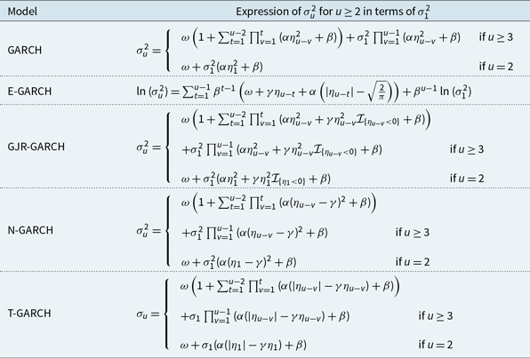
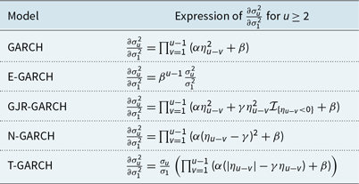
In developing the improved framework, the first step is to obtain recursive expressions of $\sigma^2_{u}$ , $u = 2, 3, \ldots$ , in terms of $\sigma^2_1$ , using equations (4)–(8). The expressions of $\sigma^2_{u}$ , $u = 2, 3, \ldots$ , in terms of $\sigma^2_1$ for the GARCH model as well as the four GARCH-type models that permit asymmetry in volatility are summarised in Table 6.

Table 6.

Expression of $\sigma^2_{u}$ , $u = 2,3,\ldots$ , in terms of $\sigma^2_{1}$ for all GARCH-type models under consideration.

Then, using the expressions in Table 6 and equation (14), we can express $S_{x,t}(T)$ in terms of $\kappa_0$ and $\sigma_1$ for each of the GARCH-type models we consider. Finally, noting that $\sigma^2_1$ is non-random given $\mathcal{F}_0$ , we obtain

(20) \begin{equation}p_{x,t}(T,\kappa_0,\sigma^2_1) \coloneqq \mathrm{E}[{S_{x,t}(T)|\mathcal{F}_0}]\end{equation}

as the key building block of the improved longevity Greeks framework.

4.3 Longevity vega for $p_{x,t}(T,\kappa_0,\sigma^2_1)$

In the improved longevity Greeks framework, the longevity vega for $p_{x,t}(T,\kappa_0,\sigma^2_1)$ is obtained by taking the first-order partial derivative of $p_{x,t}(T,\kappa_0,\sigma^2_1)$ with respect to $\sigma^2_1$ :

(21) \begin{align}V_{x,t}(T) &\coloneqq \frac{\partial p_{x,t}(T,\kappa_0,\sigma^2_1)}{\partial \sigma^2_1} = \mathrm{E}\left[{\frac{\partial S_{x,t}(T)}{\partial \sigma^2_1} |\mathcal{F}_0}\right] \nonumber \\[5pt] &= \mathrm{E}\left[{\exp(-W_{x,t}(T)) \left( -\sum_{s=1}^{T}\exp(Y_{x,t}(s)) \left( b_{x+s-1} \sum_{u=1}^{t+s} \frac{\partial \sigma_{u}\eta_{u}}{\partial \sigma^2_1} \right) \right)| \mathcal{F}_0}\right] \nonumber \\[5pt] &= -\sum_{s=1}^T b_{x+s-1} \mathrm{E}\left[{\exp(Y_{x,t}(s)-W_{x,t}(T)) \left( \sum_{u=1}^{t+s} \frac{\eta_{u}}{2\sigma_{u}} \frac{\partial \sigma^2_{u}}{\partial \sigma^2_1} \right)| \mathcal{F}_0}\right]\end{align}

where $\frac{\partial \sigma^2_u}{\partial \sigma^2_{1}} = 1$ for $u=1$ , and $\frac{\partial \sigma^2_u}{\partial \sigma^2_{1}}$ for $u\geq2$ depends on the chosen GARCH-type model.

For the GARCH, GJR-GARCH and N-GARCH models, the expression of $\frac{\partial \sigma^2_u}{\partial \sigma^2_{1}}$ for $u\geq2$ can be easily derived from the corresponding expressions of $\sigma^2_u$ for $u\geq2$ in Table 6. For the E-GARCH model, we use the chain rule to get

\[\frac{\partial \sigma^2_t}{\partial \sigma^2_{1}} = \frac{\partial \sigma^2_t}{\partial \ln(\sigma^2_{t})} \frac{\partial \ln(\sigma^2_t)}{\partial \ln(\sigma^2_{1})} \frac{\partial \ln(\sigma^2_1)}{\partial \sigma^2_{1}} = \frac{\sigma^2_{t}}{\sigma^2_{1}} \frac{\partial \ln(\sigma^2_t)}{\partial \ln(\sigma^2_{1})} \]

where 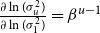$\frac{\partial \ln(\sigma^2_u)}{\partial \ln(\sigma^2_{1})}=\beta^{u-1}$ for $u\geq2$ can be obtained straightforwardly from the expression of $\sigma^2_u$ for $u\geq2$ for the E-GARCH model as shown in Table 6. Lastly, for the T-GARCH model, the chain rule is used to get

\[\frac{\partial \sigma^2_u}{\partial \sigma^2_{1}} = \frac{\partial \sigma^2_u}{\partial \sigma_u} \frac{\partial \sigma_u}{\partial \sigma_1} \frac{\partial \sigma_1}{\partial \sigma^2_{1}} = \frac{\sigma_{u}}{\sigma_{1}} \frac{\partial \sigma_u}{\partial \sigma_1}\]

where $\frac{\partial \sigma_u}{\partial \sigma_1}=\prod_{v=1}^{u-1} (\alpha(|\eta_{u-v}| - \gamma\eta_{u-v}) + \beta)$ for $u\geq2$ can be derived from the expression of $\sigma^2_u$ for $u\geq2$ for the T-GARCH model as shown in Table 6. The resulting expressions of $\frac{\partial \sigma^2_u}{\partial \sigma^2_{1}}$ for $u \geq 2$ for all GARCH-type models under consideration are presented in Table 7.

Table 7.

Expressions of $\frac{\partial \sigma^2_u}{\partial \sigma^2_{1}}$ , $u = 2,3, \ldots$ , for all GARCH-type models under consideration.

The expressions of both $Y_{x,t}(s)$ and $W_{x,t}(T)$ in equation (21) also depend on the chosen GARCH-type model. In particular, they depend on $\sigma^2_u$ for $u \geq 2$ (which in turn depends on the GARCH-type model chosen) through equations (11), (12) and (13). The calculation of $Y_{x,t}(s)$ and $W_{x,t}(T)$ is enabled by the expressions provided in Table 6.

Let us revisit the longevity vega under the GARCH model assumption. From Table 7 and equation (21), we observe that in the improved framework the longevity vega under the GARCH model assumption is non-zero unless both $\alpha$ and $\beta$ are zero (which happens only when $\sigma^2_t$ is indeed a constant), suggesting that the spurious zero vega problem found in the original longevity Greeks framework of Zhou & Li (Reference Zhou and Li2019a) is mitigated. This desirable property also applies to all other GARCH-type models under consideration except the E-GARCH, for which the longevity vega must be zero if $\beta = 0$ regardless of whether or not $\alpha$ is zero.

4.4 Longevity delta and gamma for $p_{x,t}(T,\kappa_0,\sigma^2_1)$

As the partial derivatives of $p_{x,t}(T,\kappa_0,\sigma^2_1)$ and $p_{x,t}(T,\kappa_0,\sigma^2_0)$ with respect to $\kappa_0$ are identical, longevity delta and gamma in the improved framework remain the same as those in the original framework of Zhou & Li (Reference Zhou and Li2019a). They are reported below for completeness.

The longevity delta for $p_{x,t}(T,\kappa_0,\sigma^2_1)$ is

(22) \begin{equation}\Delta_{x,t}(T) \coloneqq \frac{\partial p_{x,t}(T,\kappa_0,\sigma^2_1)}{\partial \kappa_0} = -\sum_{s=1}^T b_{x+s-1} \mathrm{E}[{\exp(Y_{x,t}(s)-W_{x,t}(T)) | \mathcal{F}_0}]\end{equation}

and the longevity gamma for $p_{x,t}(T,\kappa_0,\sigma^2_1)$ is

(23) \begin{align}\Gamma_{x,t}(T) &\coloneqq \frac{\partial^2 p_{x,t}(T,\kappa_0,\sigma^2_1)}{\partial \kappa_0^2} \nonumber \\&= \mathrm{E}\left[{\exp(-W_{x,t}(T)) \left( \left( \sum_{s=1}^T b_{x+s-1}\exp(Y_{x,t}(s))\right)^2 - \sum_{s=1}^T b^2_{x+s-1}\exp(Y_{x,t}(s)) \right) | \mathcal{F}_0}\right]\end{align}

As discussed in the previous subsection, $Y_{x,t}(s)$ and $W_{x,t}(T)$ in the above expressions depend on the chosen GARCH-type model.

4.5 Additional remarks

We compute the values of $\Delta_{x,t}(T)$ , $\Gamma_{x,t}(T)$ and $V_{x,t}(T)$ with simulations. In particular, using N simulated paths of $\{\eta_s;\, s=1,\dots,t+T\}$ , we calculate N realisations of $Y_{x,t}(s)|\mathcal{F}_0$ , $W_{x,t}(T)|\mathcal{F}_0$ and $\frac{\partial \sigma^2_u}{\partial \sigma^2_1}|\mathcal{F}_0$ for $u\geq2$ , with which the expectations in equations (1), (22) and (23) can be evaluated.

The values of annuity/pension liabilities and typical mortality-linked instruments can be expressed as linear combinations of $p_{x,t}(T,\kappa_0,\sigma^2_1)$ for different values of x, t and T. As such, their longevity Greeks can be expressed as linear combinations of $\Delta_{x,t}(T)$ , $\Gamma_{x,t}(T)$ or $V_{x,t}(T)$ for different values of x, t and T. The calculation of longevity Greeks for the values of liabilities and instruments is illustrated in sections 6.2 and 6.3.

6.1 General assumptions

The following assumptions are used in both illustrations.

• The liability being hedged is a pension plan for pensioners who are all aged 60 years at time 0. The plan pays each pensioner $1 at the end of each year until death or age 90 years, whichever is the earliest. The mortality experience of the pensioners is identical to that of the Italian female population. The plan contains an infinitely large number of pensioners, so diversifiable risk can be ignored.

• The hedger establishes a Greek longevity hedge for the pension plan using a S-forward at time 0. No adjustment is made to the hedge after time 0.

• At time 0, freshly launched S-forwards with a reference age 60 years and times-to-maturity from 1 to 20 years are available. The hedger uses S-forwards of which the reference population is Italian female, so there is no population basis risk. Further information about S-forwards is given in section 6.3.

• The evaluation of hedge effectiveness is based on the E-GARCH(1,1) model, which, as shown in section 2, is found to be the best fitting model for the Italian female population. Parameter estimates of the E-GARCH(1,1) model fitted to the data from the Italian female population (over ages 40 to 89 and years 1900 to 2014) are reported in Table 8.

• Time 0 is defined as the end of year 2014 (i.e., the end point of the calibration window).

• When discounting future cash flows, an interest rate of $r=3\%$ per annum for all durations is used.

6.2 Longevity Greeks for the liability being hedged

We now derive the longevity Greeks of the value of the pension plan. As per the assumptions made, we have

\[ \mathcal{L} = \sum_{s=1}^{30}(1+r)^{-s} S_{60,0}(s) \]

as the sum of all future cash flows (per pensioner), discounted to time 0. Given $\mathcal{F}_0$ , $\mathcal{L}$ is a random variable which depends on the evolution of mortality between time 1 and time 30. It follows that on a per pensioner basis, the time-0 value of the plan is

\[L(\kappa_0,\sigma^2_1) \coloneqq \mbox{E}[\mathcal{L} | \mathcal{F}_0] = \sum_{s=1}^{30}(1+r)^{-s}p_{60,0}(s,\kappa_0,\sigma^2_1) \]

As $L(\kappa_0,\sigma^2_1)$ is a linear combination of $p_{60,0}(s,\kappa_0,\sigma^2_1)$ for different values of s, the longevity Greeks of $L(\kappa_0,\sigma^2_1)$ can be calculated straightforwardly using the results in sections 4 and 5. The longevity delta, longevity gamma, longevity vega and dynamic delta of $L(\kappa_0,\sigma^2_1)$ are given by

\begin{align*}\Delta^{(L)} &\coloneqq \frac{\partial L(\kappa_0,\sigma^2_1)}{\partial \kappa_0} = \sum_{s=1}^{30} (1+r)^{-s} \Delta_{60,0}(s) \\[1pt] \Gamma^{(L)} &\coloneqq \frac{\partial^2 L(\kappa_0,\sigma^2_1)}{\partial \kappa^2_0} = \sum_{s=1}^{30} (1+r)^{-s} \Gamma_{60,0}(s) \\[1pt] V^{(L)} &\coloneqq \frac{\partial L(\kappa_0,\sigma^2_1)}{\partial \sigma^2_1} = \sum_{s=1}^{30} (1+r)^{-s} V_{60,0}(s)\end{align*}

and

\begin{align*}\Lambda^{(L)} & \coloneqq \frac{d L(\kappa_0,\sigma^2_1)}{d \kappa_0} = \sum_{s=1}^{30} (1+r)^{-s} \Lambda_{60,0}(s)\end{align*}

respectively.

6.3 Longevity Greeks for the hedging instrument

Here, we derive the longevity Greeks of the value of a S-forward. A S-forward is a zero-coupon swap with a fixed leg proportional to a forward survival rate $S^{\;f}$ that is predetermined at inception, and a floating leg proportional to a (random) realised survival rate. For a S-forward with a time-to-maturity of $t^{\;f}$ and a reference age of $x^{\;f}$ , the realised survival rate is the one for individuals aged $x^{\;f}$ when the S-forward is launched over a period of $t^{\;f}$ years. To mitigate longevity risk, a hedger can participate in a S-forward as a fixed-rate payer, so that when future mortality turns out to be lighter than expected (i.e., the realised survival rate turns out to be lower than expected), the hedger will receive from the counterparty a positive net payment, which can be used to offset the correspondingly higher pension/annuity liability.

From the fixed-rate payer’s perspective, the pay-off of a S-forward (with a reference age of $x^{\;f} = 60$ years and an issue date of $t=0$ ) discounted to time 0 is

\begin{align*}\mathcal{H} &= (1+r)^{-t^{\;f}}(S_{60,0}(t^{\;f})-S^{\;f})\end{align*}

per $1 notional. Given $\mathcal{F}_0$ , $\mathcal{H}$ is a random variable which depends on the evolution of mortality between time 1 and time $t^{\;f}$ . It follows that the time-0 value of the S-forward is

\begin{equation*}H(\kappa_0,\sigma^2_1) \coloneqq \mbox{E}[\mathcal{H} | \mathcal{F}_0] = (1+r)^{-t^{\;f}}(p_{60,0}(t^{\;f},\kappa_0,\sigma^2_1) - S^{\;f})\end{equation*}

per $1 notional.

As $H(\kappa_0,\sigma^2_1)$ is linearly related to 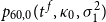$p_{60,0}(t^{\;f},\kappa_0,\sigma^2_1)$ , the longevity Greeks of $H(\kappa_0,\sigma^2_1)$ can be obtained easily using the results in section 4 and 5. The longevity delta, longevity gamma, longevity vega and dynamic delta of $H(\kappa_0,\sigma^2_1)$ are given by

\begin{align*}\Delta^{(H)} &\coloneqq \frac{\partial H(\kappa_0,\sigma^2_1)}{\partial \kappa_0} = (1+r)^{-t^{\;f}} \Delta_{60,0}(t^{\;f}) \\ \Gamma^{(H)} &\coloneqq \frac{\partial^2 H(\kappa_0,\sigma^2_1)}{\partial \kappa^2_0} = (1+r)^{-t^{\;f}} \Gamma_{60,0}(t^{\;f}) \\ V^{(H)} &\coloneqq \frac{\partial H(\kappa_0,\sigma^2_1)}{\partial \sigma^2_1} = (1+r)^{-t^{\;f}} V_{60,0}(t^{\;f})\end{align*}

and

\begin{align*}\Lambda^{(H)} &\coloneqq \frac{d H(\kappa_0,\sigma^2_1)}{d \kappa_0} = (1+r)^{-t^{\;f}} \Lambda_{60,0}(t^{\;f})\end{align*}

respectively.

The longevity Greeks of a S-forward do not depend on its forward survival rate $S^{\;f}$ , because $S^{\;f}$ is predetermined at time 0 and is thus treated as a constant. We set $S^{\;f}$ to 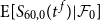$\mbox{E}[S_{60,0}(t^{\;f}) | \mathcal{F}_0]$ , a forward survival rate which implies that no payment exchanges hands at time 0 (i.e., $\mbox{E}[\mathcal{H} | \mathcal{F}_0]=0$ ).

6.4 Hedge calibration

A Greek longevity hedge can be created by matching the longevity Greek(s) of the liability being hedged and the hedging instrument(s). The longevity hedges in both of our illustrations are calibrated by matching dynamic delta, the new longevity Greek proposed in this paper.

Since we are matching one longevity Greek, only one S-forward is needed. When the dynamic deltas of the liability being hedged and the S-forward are matched, the notional amount of the S-forward is calculated at time 0 as

\begin{equation*}u = \frac{\Lambda^{(L)}}{\Lambda^{(H)}}\end{equation*}

To demonstrate the impact of asymmetry in mortality volatility on the longevity hedges, we calculate two sets of results which respectively represent the situations when asymmetry in mortality volatility is ignored and taken into account:

1. (I) Asymmetry in mortality volatility is ignored

   For this set of results, the longevity Greeks (and hence the notional amount u) are derived from a GARCH(1,1) model, which does not permit volatility to respond asymmetrically to positive and negative shocks. The GARCH(1,1) model is fitted to the Italian female data described in section 6.1. The forward survival rate $S^{\;f}$ is also calculated from the GARCH(1,1) model to mimic the situation when participants in the S-forward market ignore any asymmetry in mortality volatility. However, the mortality scenarios used to evaluate hedge effectiveness are generated from the E-GARCH(1,1) model as described in section 6.1 to reflect the fact that asymmetry in mortality volatility exists.

2. (II) Asymmetry in mortality volatility is taken into account

   In line with the model from which the mortality scenarios for evaluating hedge effectiveness are generated, the longevity Greeks (and hence the notional amount u) as well as the forward survival rate $S^{\;f}$ for this set of results are calculated from the E-GARCH(1,1) model which permits asymmetry in mortality volatility.

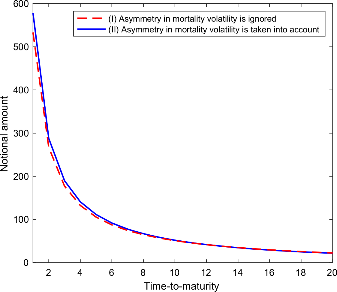
Figure 3 shows the resulting S-forward notional amounts u under both scenarios. For short-term S-forwards, the notional amounts calculated when asymmetry in mortality volatility is ignored are smaller than those calculated when asymmetry in mortality volatility is taken into account. The difference diminishes as the S-forward time-to-maturity increases.

Figure 3

Notional amounts of S-forwards with times-to-maturity ranging from 1 to 20 years, calculated when (I) asymmetry in mortality volatility is ignored (dashed red line) and when (II) asymmetry in mortality volatility is taken into account (solid blue line).

6.5 Illustration 1: value hedge

The first illustration concerns a value hedge, which aims to reduce the variability of the values of the pension plan sponsor’s position at time 1. We measure hedge effectiveness by the reduction in the 1-year ahead 99.5% Value-at-Risk over the time-0 value of the unhedged position:

\begin{equation*}1 - \frac{\mbox{VaR}_{99.5\%}\left(\mbox{E}[\mathcal{L}-u\mathcal{H}|\mathcal{F}_1] | \mathcal{F}_0\right) - \mbox{E}[\mathcal{L}|\mathcal{F}_0]}{\mbox{VaR}_{99.5\%}(\mbox{E}[\mathcal{L}|\mathcal{F}_1] | \mathcal{F}_0) - \mbox{E}[\mathcal{L}|\mathcal{F}_0]}\end{equation*}

The following comments concerning this metric of hedge effectiveness are made.

• In the expression, $\mathcal{L}$ is the pension plan sponsor’s position in the absence of a longevity hedge. Measured in time-0 dollars, the time-0 and time-1 values of the position are $\mbox{E}[\mathcal{L}|\mathcal{F}_1]$ and $\mbox{E}[\mathcal{L}|\mathcal{F}_0]$ , respectively.

• In the numerator of the expression, $\mathcal{L}-u\mathcal{H}$ is the pension plan sponsor’s position when the longevity hedge is in place. Measured in time-0 dollars, the time-1 value of the position is $\mbox{E}[\mathcal{L}-u\mathcal{H}|\mathcal{F}_1]$ .

• Given $\mathcal{F}_0$ , $\mbox{E}[\mathcal{L}|\mathcal{F}_1]$ and $\mbox{E}[\mathcal{L}-u\mathcal{H}|\mathcal{F}_1]$ are random variables depending on the unknown realisation of $\mathcal{F}_1$ , but $\mbox{E}[\mathcal{L}|\mathcal{F}_0]$ is a known constant.

• If the value hedge is effective, then the value of the metric should be close to one; if the opposite is true, then the value of the metric should be close to zero.

We use nested simulations to calculate the value of the metric. In more detail, we first use the fitted E-GARCH model to generate 10,000 mortality scenarios at time 1 (i.e., 10,000 realisations of $\mathcal{F}_1$ ). For each of these mortality scenarios, another 10,000 mortality scenarios are generated (also using the fitted E-GARCH model) to compute 10,000 realisations of $\mbox{E}[\mathcal{L}|\mathcal{F}_1]$ and $\mbox{E}[\mathcal{H}|\mathcal{F}_1]$ , from which empirical distributions of $\mbox{E}[\mathcal{L}-u\mathcal{H}|\mathcal{F}_1]$ and $\mbox{E}[\mathcal{L}|\mathcal{F}_1]$ given $\mathcal{F}_0$ are obtained. The 99.5th percentiles of these two empirical distributions give the estimated 99.5% Values-at-Risk of $\mbox{E}[\mathcal{L}-u\mathcal{H}|\mathcal{F}_1]$ and $\mbox{E}[\mathcal{L}|\mathcal{F}_1]$ , respectively. Lastly, $\mbox{E}[\mathcal{L}|\mathcal{F}_0]$ is calculated with non-nested simulations.

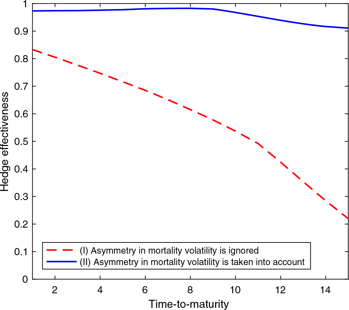
Figure 4 compares the effectiveness of the value hedges that are calibrated when (I) asymmetry in mortality volatility is ignored and when (II) asymmetry in mortality volatility is taken into account. When asymmetry in mortality volatility is incorporated into the calibration of the value hedge, the hedge effectiveness ranges between 0.9 and 1, indicating that the hedge reduces at least 90% of the 99.5% Value-at-Risk over a horizon of 1 year. If the hedger ignores asymmetry in mortality volatility, then the hedge effectiveness is significantly reduced (by up to 70% points depending on the time-to-maturity of the S-forward used).

Figure 4

Effectiveness of the value hedges that are calibrated when (I) asymmetry in mortality volatility is ignored (dashed red line) and when (II) asymmetry in mortality volatility is taken into account (solid blue line), for S-forward times-to-maturity ranging from 1 to 15 years.

6.6 Illustration 2: cash flow hedge

The second illustration concerns a cash flow hedge, which aims to reduce the variability of all future cash flows of the pension plan sponsor. In this illustration, we measure hedge effectiveness by the reduction in the 99.5% Value-at-Risk of all future cash flows measured in time-0 dollars over the time-0 value of the liability being hedged:

\begin{equation*}1 - \frac{\mbox{VaR}_{99.5\%}\left( \mathcal{L}-u\mathcal{H} | \mathcal{F}_0\right) - \mbox{E}[\mathcal{L}|\mathcal{F}_0]}{\mbox{VaR}_{99.5\%}( \mathcal{L} | \mathcal{F}_0) - \mbox{E}[\mathcal{L}|\mathcal{F}_0]}\end{equation*}

where $\mathcal{L}-u\mathcal{H}$ and $\mathcal{L}$ represent the present (time-0) value of all cash flows arising from the hedged and unhedged positions, respectively. If the cash flow hedge is effective, then the value of the metric should be close to one; if the opposite is true, then the value of the metric should be close to zero.

To compute the value of the metric defined above, we use the fitted E-GARCH model to generate 10,000 realisations of $\mathcal{L}$ and $\mathcal{H}$ , from which empirical distributions of $\mathcal{L}-u\mathcal{H}$ and $\mathcal{L}$ given $\mathcal{F}_0$ are obtained. The 99.5th percentiles of these two empirical distributions give the estimated 99.5% Values-at-Risk of $\mbox{E}[\mathcal{L}-u\mathcal{H}|\mathcal{F}_0]$ and $\mbox{E}[\mathcal{L}|\mathcal{F}_0]$ , respectively. As in the first illustration, $\mbox{E}[\mathcal{L}|\mathcal{F}_0]$ is also calculated with non-nested simulations.

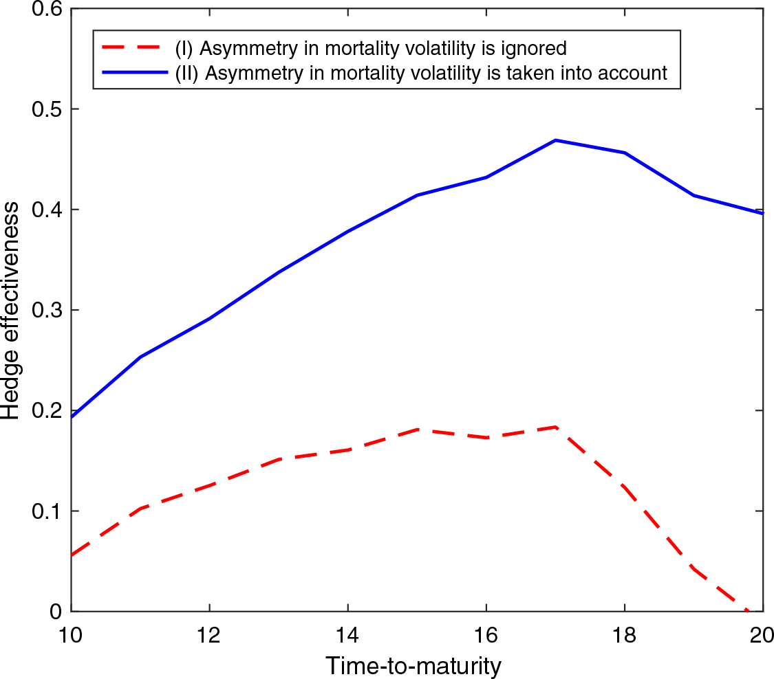
Figure 5 compares the effectiveness of the cash flow hedges that are calibrated when (I) asymmetry in mortality volatility is ignored and when (II) asymmetry in mortality volatility is taken into account. For all S-forward times-to-maturity considered, the effectiveness of the hedge that takes asymmetry in mortality volatility into account is higher compared to the hedge that ignores asymmetry in mortality volatility. The difference in hedge effectiveness ranges from 10% to 40% points, depending on the time-to-maturity of the S-forward used.

Figure 5

Effectiveness of the cash flow hedges that are calibrated when (I) asymmetry in mortality volatility is ignored (dashed red line) and when (II) asymmetry in mortality volatility is taken into account (solid blue line), for S-forward times-to-maturity ranging from 10 to 20 years.