2. f-SWAP RULES

Consider the following family of f-swap rules: If the successful attempt of a path is in position j, j = 1,2,…,n, then this path exchanges its position with the path in position f (j), where f is a given mapping from the set {1,2,…,n} into itself. The mapping f can be represented by a directed graph with every vertex having out-degree unity. Throughout this section we will assume that the graph has exactly one directed cycle. Under this assumption, we will generalize the result about the stationary distributions in Lam and Cowan [7].

Let R be all the vertices in the unique directed cycle of the graph. Define

For a position j ∈ A ∪ B, let g(j) be the generation number of j (i.e., the smallest number of mappings applied such that f ○ f ○ … ○ f (j) ∈ R). For j ∈ R, let g(j) = 0. Furthermore, let

for j ∈ A ∪ B and w(j) = 0 for j ∈ R.

For convenience we will let q_j = 1 − p_j, a_j = p_j /q_j and

which represents the routing table immediately preceding the routing table π when a call is completed through the path in position k. We will also make use of the conventions that for any function F,

The following lemma is needed for finding the stationary distributions.

Lemma 1:

Proof: When k = n, the left-hand side of Eq. (1) is

which equals the right-hand side of Eq. (1). Now suppose that Eq. (1) is true when k = K + 1. Then when k = K, by assumption of induction

Hence, Eq. (1) is true when k = 1,2,…,n. █

Theorem 1: Under the swap-forward rule with

the stationary probability of state π is proportional to

Especially when z = 1 and f (k) = k − 1 for k ≥ 2, the swap-forward rule becomes the transposition rule and the stationary probability of state π is proportional to

(see Chong and Lam [2]).

Proof: First note that g(f (k)) = g(k) − 1 for k ∈ A ∪ B and

Let

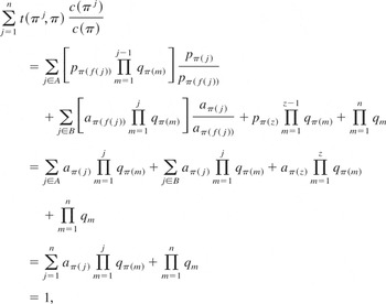
where the last equality is due to Lemma 1. Hence,

.

Example 1: Suppose n = 3, f (1) = 3, f (2) = 1, and f (3) = 1. Then the transition probability from σ to (1,2,3) is

Note that g(1) = g(3) = w(1) = w(3) = 0 and g(2) = w(2) = 1. Hence, c(π) = 1/a_π(2), where c(π) is defined in the proof of Theorem 1, and

Therefore, Theorem 1 cannot be generalized to the case when R = {y,z} with |y − z| > 1.

Example 2: Suppose n = 3, f (1) = 2, f (2) = 3, and f (3) = 1. Then the transition probability from σ to (1,2,3) is

Now g(i) = w(i) = 0 for i = 1,2,3 and c(π) = 1 for all permutations π. Obviously,

Therefore, Theorem 1 cannot be generalized to the case when |R| > 2.

3. COMPARING COSTS UNDER TWO MOVE-FORWARD RULES WHEN p₂ = p₃ = … = p_n

In this section we compare the move-forward rules applied to a communication problem with the assumption that p₂ = p₃ = … = p_n. For a move-forward rule characterized by l₁,l₂,…,l_n, let

which uniquely characterizes a move-forward rule (Lam [6]).

Given that p₁ = p, p₂ = p₃ = … = p_n = r, 0 < p < 1, 0 < r < 1. Let q = 1 − p and s = 1 − r. Similar to Lam [6], the arrangement of the paths can be denoted by state i, i = 1,2,…,n, where i is the position of the unique path with success probability p. Let p_ij be the one-step transition probability from state i to state j. Then

for i = 2,3,…,n.

Let the equilibrium probability vector be (h(1),h(2),…,h(n)), H(0) be 0, and H(j) be

for j = 1,2,…,n. Then the H(j)'s satisfy

or, equivalently,

Lemma 2:

Proof: Suppose p ≥ r.

From the (n − 1)st equation of Eq. (4), we have h(n − 1)qrsⁿ⁻² = h(n)psⁿ⁻¹. Hence, h(n) ≤ h(n − 1).

Now suppose

and we need to prove h(j) ≥ h(j + 1). If k(j) = 1, the jth equation of Eq. (4) is h(j)qrs^j−1 = h(j + 1)ps^j and h(j) ≥ h(j + 1) follows. If k(j) ≥ 2, from the (j + 1)st equation of Eq. (4) we get

By the induction assumption, we have

Adding

to both sides of the sum of the above k(j) inequalities, we have

Combining with Eq. (5), we obtain

Additionally, the jth equation of Eq. (4) is

Combining Eqs. (6) and (7), we get h(j) ≥ h(j + 1), which completes the proof of part (a).

The proof of part (b) is similar to the proof of part (a).

For the proof of part (c), we make use of Eq. (7) and part (a) to obtain

Thus, h(j)qr ≥ h(j + 1)ps.

The proof of part (d) is similar to the proof of part (c). █

For state i, the expected cost, which is the expected number of paths to attempt before a call is completed or blocked, is

Thus, the expected cost corresponding to the equilibrium probability vector (h(1),h(2),…, h(n)) is

For the probability vectors b = (b(1),b(2),…,b(n)) and b′ = (b′(1),b′(2),…,b′(n)), define b [pr ] b′ if and only if

Lemma 3:

Proof: By Abel's partial summation formula,

Therefore,

. The conclusions can then be derived from the above expression for C. █

For a transition probability matrix (p_mj, m,j = 1,2,…,n), let

Lemma 4: For every move-forward rule, P_m,i ≥ P_m+1,i, m = 1,2,…,n − 1, i = 1,2,…,n.

Proof: In fact,

Corollary: For every move-forward rule, b [pr ] b′ implies bP [pr ] b′P.

Proof:

where the second equality comes from the Abel's partial summation formula and the inequality is due to b [pr ] b′ and Lemma 4. █

Theorem 2: Suppose that we have two move-forward rules characterized by {l₁,l₂,…,l_n} and {l₁′,l₂′,…,l_n′}, respectively, and l_i ≤ l_i′ for all i = 1,2,…,n. Denote their equilibrium probability vectors by h and h′, respectively, and the corresponding expected costs by C and C′. Then the following hold:

Proof: Note that l_i ≤ l_i′ for all i = 1,2,…,n is equivalent to k′(j) ≤ k(j) for all j = 1,2,…,n − 1 (Lam [6]), where the k(j)'s and k′(j)'s are defined by Eq. (2).

For the proof of part (a), suppose p ≥ r. First we will prove that h′ [pr ] h′P, where P is the transition probability matrix according to the move-forward rule with k(1),k(2),…,k(n − 1). The sum of the first i entries of h′P is given by

where H′(i) is the sum of the first i entries of h′. Note that H′(i) satisfies the ith equation of Eq. (3): that is,

Thus, D(i) ≤ H′(i), is equivalent to

Since p ≥ r, this is true by parts (c) and (a) of Lemma 2. Thus, h′ [pr ] h′P is proved. Then by the corollary to Lemma 4, h′ [pr ] h′P [pr ] h′P² [pr ] h′P³ [pr ] … and so h′ [pr ] h.

The proof of part (b) is similar to that of part (a).

For the proof of part (c), C′ ≤ C comes immediately from parts (a) and (b) and Lemma 3. █

4. COMPARING COSTS UNDER A MOVE-FORWARD RULE FOR DIFFERENT SETS OF SUCCESS PROBABILITIES

In this section, we consider only one move-forward rule and assume that there are two sets of success probabilities, p₁ = p, p₂ = p₃ = … = p_n = r and p₁ = p′, p₂ = p₃ = … = p_n = r′, where 0 < p < 1, 0 < r < 1, 0 < p′ < 1, and 0 < r′ < 1. Let P and P′ be the corresponding transition matrices and let h and h′ be the corresponding equilibrium probability vectors. Let also q = 1 − p, s = 1 − r, q′ = 1 − p′, and s′ = 1 − r′.

Lemma 5: If p ≥ p′ and r = r′, then h [pr ] h′.

Proof: Let

for m,i = 1,2,…,n, where the p_mj's and p_mj′'s are the one-step transition probabilities for the two sets of success probabilities, respectively. For any probability vectors b and b′ such that b [pr ] b′, we have bP′ [pr ] b′P′ by the corollary to Lemma 4. On the other hand, for every i = 1,2,…,n,

because P_m,i ≥ P_m,i′ for m,i = 1,2,…,n (refer to the expression for P_m,i in the proof of Lemma 4). Therefore, bP [pr ] bP′. Hence, h = hP [pr ] hP′ [pr ] h(P′)² [pr ] h(P′)³ [pr ] … and so h [pr ] h′. █

Denote the expected costs corresponding to h and h′ by C and C′, respectively.

Theorem 3: If p ≥ p′ ≥ r = r′ or p ≥ r = r′ ≥ p′, then C ≤ C′.

Proof: Suppose that p ≥ p′ ≥ r = r′. Let

Then

. Now by Abel's partial summation formula and Lemma 5,

For the case p ≥ r = r′ ≥ p′,

When r = r′ ≥ p ≥ p′, C might be greater or smaller than C′. As an example, consider cases when n = 4 and r = 0.9. For the move-to-front rule, the expected equilibrium costs are 1.11957414, 1.11957444, and 1.11957383 for p = 0.814, 0.815, and 0.816, respectively. For the POS(2) rule, the expected equilibrium costs are 1.11899514, 1.11899612, and 1.11899606 for p = 0.821, 0.822, and 0.823, respectively. For the transposition rule, the expected equilibrium costs are 1.11853856, 1.11853924, and 1.11853865 for p = 0.828, 0.829, and 0.83, respectively.