




No CrossRef data available.
INFERENCE ON SEGMENTED COINTEGRATION
Published online by Cambridge University Press: 06 June 2003
Abstract
A cointegration relation is often interpreted as a long-run equilibrium relation whereas short-run deviations are allowed to a certain extent. In practice, however, real data often fail to confirm cointegration for a well understood economic relation. This paper proposes that in many cases failure of confirming cointegration is due to nonstationary deviations in a relatively small portion of the data period (“short-run”) whereas a cointegration relation prevails in the other periods. We call such a situation segmented cointegration. We study in this paper how to detect segmented cointegration and how to identify the period of short-run deviations.I thank Pentti Saikkonen and three anonymous referees for helpful comments. I am deeply indebted to Peter Phillips for encouragement, discussion, and helpful comments on this work. The research of this paper is supported by the Research Grants Council of Hong Kong (grant HKUST6178/98H) and FRAP B of SUNY-Albany (account 320-9709W).
Information
- Type
- Research Article
- Information
- Copyright
- © 2003 Cambridge University Press
1. INTRODUCTION
The concept of cointegration defined and introduced by Engle and Granger (1987) has become a useful concept for analyzing linear dynamic systems in economics. A cointegration relation is often interpreted as a long-run equilibrium in a system of variables whereas short-run deviations are allowed to a certain extent. Therefore, the cointegration concept applies for statistical inference on many economic theories that are concerned with equilibrium relationships. In practice, however, real data often fail to confirm cointegration for a well understood economic relation.
Failure of rejection of the null of no cointegration could be explained by a variety of reasons. For example, test results are sensitive to various factors such as the span of data set (Hendry, 1995), the choice of lags in the testing equations (Banerjee, Dolado, Galbraith, and Hendry, 1993), the possibility of structural breaks in the underlying relationship (Gregory and Hansen, 1996; Hansen and Johansen, 1993; Stock and Watson, 1994), and threshold effects in a possible cointegration relation (Balke and Fomby, 1996). Siklos and Granger (1997) consider the case when the given variables are cointegrated only during some periods and not at others, which is applied for interest rate parity of the United States and Canada. Many of the preceding reasons would be related to the presence of temporary nonstationary deviations from a long-run relation.
In this paper we propose that failure of rejection of the null of no cointegration in many cases is due to nonstationary deviations in a relatively small portion of the data period (“short-run”) whereas a cointegration relation prevails in the other periods. We call such a situation segmented cointegration. This situation is possible if some important events or changes in an economy interrupt the underlying economic relation for a certain length of time.1
In this sense, the concept of segmented cointegration has much to do with structural change that occurs over several periods of time. Therefore, the approach of this paper contrasts with most of the existing works in the literature of structural change, which are about structural break(s) that all occur at single period(s) of time. (See Hansen and Johansen, 1993, and references therein.) A segmented cointegration, however, can result from situations other than structural change.
We study in this paper how to detect segmented cointegration and how to identify the period of short-run deviations. An idea for detecting a segmented cointegration is to use a test for testing the null of no cointegration for each of the two regressions, one regression based on the sample without segmentation and the other based on the sample with segmentation. The regression based on segmentation is a special case of the weighted least square, which is the only way of getting a consistent estimator under the alternative of segmented cointegration. As the period of noncointegration is unknown in practice, we search over a set of all possible segmentations. If there exists a segmentation for which the null is rejected whereas the null is not rejected for the sample without segmentation, we can conclude that the basic cointegration relation prevails in the sample with the segmentation. The actual testing procedure is to determine whether the smallest value of a statistic over a set of possible segmentations falls in a critical region. The reason for using the smallest value of a test statistic is that it constitutes evidence against the null hypothesis. As shown in Section 3, the tests based on segmentation are consistent tests. Monte Carlo simulation is performed for exploring performance of the procedures for detecting segmented cointegration. For identifying the period of noncointegration we propose an extremum estimator. We show that the estimator is a consistent estimator with T-rate of convergence. Alternatively, the noncointegration period can be identified by the period that corresponds to the segmentation yielding the minimum value of the test statistic for testing the existence of segmented cointegration.
The paper is organized as follows. Section 2 introduces definitions and assumptions. Also, Section 2 explains why real data often fail to confirm a cointegration relation in the presence of short-run deviations. Section 3 discusses how to detect segmented cointegration and how to locate the period of noncointegration. A set of Monte Carlo results is provided in Section 4. Section 5 concludes the paper.
2. PRELIMINARIES
2.1. Basic Concepts and Notations
Let x1t be a scalar I(1) process and x2t be an (n − 1) vector I(1) process. Suppose that these variables have one of the following relations:


Define the innovation vector ut = Δxt or ut = Δxt − γ in the presence of some trending variable(s). Also, define its cumulative process

and its long-run variance Ω = limT T−1EST ST′. We use the following regularity conditions.
Assumption 1.
(a) {ut} is mean-zero and strong mixing with mixing coefficient of size −rκ/(r − κ), and E|ut|r < ∞ for some

.
(b) The matrix Ω exists with finite elements and is positive definite.
(c) x0 is a random vector with E|x0| < ∞.
The conditions in Assumption 1 allow a broad class of weakly dependent time series and have been used by Phillips (1987), Phillips and Perron (1988), Phillips and Ouliaris (1990), and Gregory and Hansen (1996), among others, to study limiting behavior of some stochastic processes.
Now, consider the possibility that the error term εt is a unit root process in a subset of the data period, whereas it may follow a stationary process for the rest of the data period. We reserve notation for these two different types of periods,

, respectively. We assume that

consists of a single interval of periods. More specifically,

for two time periods k0 and k1, k0 < k1.
Assumption 2. Let

be the number of elements in

. We assume that

.
Assumption 2 rules out the case of a “trivial” segmented cointegration with

: for example, for n = 2 if

then any process forms a segmented cointegration by defining β = x1h /x2h and εh = 0 for each h = 1,…,T.
When

consists of more than one interval of periods, we need to determine the number of segmentations in practice. Formal analysis of the problem of multiple segmentations is beyond the scope of this paper. However, we briefly discuss this problem in Section 3.
Testing for cointegration for (2.1) is often based on testing for the null of no cointegration. Thus, writing the disturbance process as an AR(1):

the hypotheses are for the value of ρ: the null of ρ = 1 vs. |ρ| < 1. There are several different tests for testing such hypotheses, that is, Dickey–Fuller (1979) tests, Phillips (1987) tests, Phillips and Perron (1988) tests, Phillips and Ouliaris (1990) tests, and augmented Dickey–Fuller tests.
In the case of possible segmented cointegration we can consider the following hypotheses:

where

.
As an example of the situation implied in H1 we can consider an economy that runs in two different regimes. For example, when the monetary authority changes the policy regime from targeting the interest rate to targeting money volume, the interest rate may be stationary only in the first regime.
A situation similar to that in H1 is found in the following model of threshold cointegration studied in Balke and Fomby (1996), among others:

When the “threshold” θ is a sufficiently small constant, then the preceding process εt is effectively a stationary process as is the case in Balke and Fomby (1996). However, if the threshold θ is not a small number or is a random variable, which sometimes has high values, the process εt may effectively be nonstationary. On the other hand, there is an important difference between segmented cointegration and threshold cointegration: segmented cointegration assumes a deterministic interval of cointegration whereas threshold cointegration depends on the conditional variables.
2.2. Failure to Confirm a Cointegration Relation
In this subsection we briefly examine why usual tests fail to confirm cointegration in the presence of short-run nonstationary deviations. To see this consider an example of the system (2.1a) under H1 where εt is such that


where

for two time periods k0 and k1, k0 < k1.
A trivial reason for the failure of confirming cointegration in the presence of short-run deviations is that the cointegrating vector may not be consistently estimated. This is because the short-run nonstationary deviations dominate in the estimate of the cointegrating vector, which very likely makes the regression spurious. If the cointegrating vector is not correctly estimated, the residual contains nonstationary regressors: in (2.1a) if

then the residual et becomes

In the presence of short-run nonstationary deviations, however, even when the cointegrating vector is known or is correctly estimated, the chance of failure of confirming cointegration of usual tests can be very high. Thus, suppose that β is known in (2.1a). Then, the simple Dickey–Fuller t-statistic for testing the null H0 (2.3) is

where

. But, since

and

, the preceding t-statistic becomes

where

, the number of elements in

, replaces T in the t-statistic. Therefore, the behavior of the t-statistic in (2.8) under H1 for the model (2.5) and (2.6) is arbitrarily close to that under H0 (2.3). In fact, under the condition that E|εk0| < ∞ asymptotic behavior of the t-statistic (2.8) is the same as that under H0. But, for t = k0 in a stationary regime the condition E|εk0| < ∞ is not restrictive. As a consequence, the statistic (2.7) would very often fail to reject H0 under H1.
3. INFERENCE ON SEGMENTED COINTEGRATION
First, we study how to detect segmented cointegration defined in the previous section. Then, we discuss how to locate the period of noncointegration.
3.1. Detection of Segmented Cointegration
When the error term in a linear regression model such as (2.1) is heterogeneous across different periods, econometric theory suggests estimating the model by a weighted least square rather than by the ordinary least square:

where wt is a weight given to the t-period residual and w = (w1,…,wT). For the model (2.1) with εt having the property in H1 the weight series {wt} should be such that

where wt = 1 for

can be replaced by wt = constant.
2The specification (3.2) for wt is justified by the following reasons: first, the data in

are not informative at all for estimating the coefficient β because in

there does not exist a β that yields stationary εt. Second, in the case of variance heterogeneity the weight wt is the reciprocal of the “variance” of εt. The reciprocal of the “variance” is arbitrarily small for

because the sample “variance” of εt in

as the relation is a spurious regression in

, which is by virtue of Phillips (1986).

for a trial period for segmented cointegration and also for the true period of segmented cointegration, regarding which the reader should not be confused. Under H0 the regression (2.1) is spurious for any choice of {wt} or

. Also, under H1 the regression yields a consistent estimator of the parameter for a proper choice of {wt} or

. For this reason a test for segmented cointegration based on the estimation (3.1) with {wt} (3.2) would have desirable properties.
Notice that the weighting process {wt} depends on the selection of

. Thus, we denote it by

. Also, denote by

, respectively, the estimator of β and the residual from (3.1) based on the weight

for a segmentation

. Let

be the least square estimator of the first-order serial correlation coefficient ρ of et in et = ρet−1 + νt for

be the t-test of ρ = 1. That is,

is obtained from regressing

on

. Also, let

be the least square variance of

be the least square estimate of the variance of the second stage residual:

where

is the number of elements of

. Define


where

, respectively, are estimators of

.
Consistent nonparametric estimators of λ and γ0 under H1 are obtained as in the following expressions:

The approach given above is based on an AR(1) for the residual process et. Alternatively, we can consider the following variant of an augmented Dickey–Fuller expression for et:

where {εt} is an independent and identically distributed (i.i.d.) sequence with mean zero, finite variance σε2, and finite fourth moment. Notice that in (3.5) the error correction term (ρ − 1)et−1 is multiplied by the “weight” wt. Let

, respectively, be the least square estimator of ρ in (3.5) and the t-test of ρ − 1 = 0.
3The initial condition et0−j for j = 1,…,p for the starting period t0 in

can be taken either from the last p observations of the previous noncointegration regime or from the first p observations of

depending on which of the two hypotheses, H0 or H1, is favored. To be in favor of H0 it can be taken from the last p observations of the previous noncointegration regime:

. To be in favor of H1 we can take the first p observations of

for the initial condition.


where

is consistently estimated by

where

is the least square estimator of ζj in (3.5).
Let

be a fixed subset of [0,1] such that

where [·] is the integer part of ·. Likewise,

. Since

consists of a single interval of periods, we may write it as

for some

where

.
Now, for a given

, the statistics

converge to some limits given in the following theorem.
THEOREM 1. Assume the conditions in Assumption 1. Under H0 it is true that


where

are such that


where

where W1(·) is a standard Wiener process and W2,m(·) depends on the model. If the residuals are from ordinary least squares (OLS) estimation of the model (2.1a), then

where W2(·) is the (n−1)-dimensional standard Wiener process. If the residuals are from OLS estimation of the model (2.1b), then

If the residuals are from OLS estimation of the model (2.1c), then

In practice, the period

is not known. In this case we adopt the following approach: we get values of the statistic

for all the possible candidates of

and take the smallest value of the statistic. The smallest value constitutes evidence against the null hypothesis.
THEOREM 2. Denote by

, etc. Assume the conditions in Assumption 1. Then, under H0 it is true that


Asymptotic critical values of these statistics can be obtained by simulating test statistics for a large sample size for a large number of replications. Because computation in the simulation for the present example for large samples is very time consuming we adopt a procedure due to MacKinnon (1991): using 10,000 replications for each of the sample sizes T = 50, 70, 100, 120, 150, 170, 200, 220, 250, 270, and 300 we obtain critical values Crt(T,p,n), where p is the percentile. We then estimate by OLS for each p and n the response surface

Various polynomials were tried (involving T−3, T−4, etc.), but the one given above appeared to be the best fit overall (R2's were generally over 0.98). The asymptotic critical value is taken to be the OLS estimate

. Although the above specification seemed to be the best overall, estimates of ψ0 changed on occasion by a factor of 2 under alternative specifications. Also, we get the critical values of

for some given upper limit of the length of

denoted by

.
4This is again to reduce the computational requirements. In practice the length of the noncointegration period

is variable, and we need critical values for each

, which are almost impossible to obtain. Fortunately, however, for a conservative test we can get an upper limit

to get the critical values (Lemma 1 in Sect. 3).

where

is the length of the interval

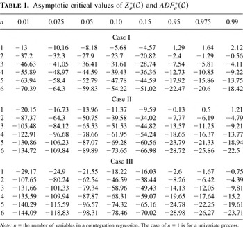
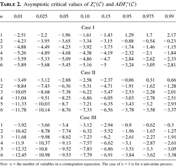
. In Tables 1 and 2 asymptotic critical values of the minimum statistics in (3.13) and (3.14) are provided for

. In Tables 1 and 2, Case I is for the model (2.1a), Case II is for the model (2.1b), and Case III is for the model (2.1c).
Asymptotic critical values of Zρ*(C) and ADFρ*(C)

Asymptotic critical values of Zt*(C) and ADFt*(C)

In practice, critical values depend on the value of

chosen for simulation. We can show that the critical value for a given size of the test is a decreasing function of

.
LEMMA 1. Let

. Denote by

the lower α-size critical value of

obtained based on

. Then, it is true that

.
Therefore, the test (3.13) or (3.14) based on critical values

for a given [ell ]2 is a conservative test when the actual test statistic

is computed for [ell ]1 such that [ell ]1 < [ell ]2.
5In general, as the assumed length of the noncointegration period is smaller the distribution of the test statistic is more concentrated, which makes the test more conservative. This is true with respect to the absolute length of the noncointegration period as well as the relative length of the noncointegration period

. Thus, for a small sample analysis the test based on asymptotic critical values would lead to conservative inference.
As was explained in Section 2, we consider in this paper the case when

consists of a single interval of periods. In practice a researcher would have situations where the number of such intervals is possibly more than one. In this case the researcher would have to determine the number of such intervals. Formal analysis of the problem of multiple segmentations including determination of the number of such intervals is beyond the scope of this paper. However, in this case we could suggest adopting the idea of detecting one by one as in Bai (1997). To describe it briefly, the approach is to divide the sample into several successive subsamples and detect the existence of segmented cointegration in each subsample based on the approach discussed in this section. This approach would save us a lot of computation time for detecting multiple intervals of noncointegration periods when the number of such intervals is unknown.
The tests for segmented cointegration

are consistent tests, which is shown by the following lemma.
LEMMA 2. Let {xt}, xt = (x1t, x2t′)′, be an n-vector I(1) process where x2t, an (n − 1) vector I(1) process, has a positive definite long-run variance-covariance matrix

. Suppose that εt = x1t − β′x2t is I(0) in a subset of data

where εt has a continuous spectral density fεε with fεε(0) > 0 in

. Then,

A Monte Carlo result in Section 4 shows that empirical power values of the tests (3.13) and (3.14) are quite high for a 5% test and for T = 200.
Remark. A model related to the one in our alternative hypothesis (2.4) has been considered by Leybourne, McCabe, and Tremayne (1996) and McCabe and Tremayne (1995):

where ρt is assumed to be an independent process. McCabe and Tremayne (1995) study how to determine whether or not the null of nonstationarity, ρt = 1, is rejected against the alternative of the root being independently changing, and Leybourne, McCabe, and Tremayne (1996) provide some applications of McCabe and Tremayne (1995). In our approach the model for alternative hypothesis is a special case of that in McCabe and Tremayne. However, the model for our alternative hypothesis allows richer statistical inference than that of McCabe and Tremayne: First, our alternative allows us to analyze a cointegration relation as well as observable individual series whereas the alternative of McCabe and Tremayne is adequate only for analyzing the latter as ρt in McCabe and Tremayne has to be an independent process. Second, our approach allows us to identify the two distinct periods, the period of noncointegration (nonstationarity) and the period of cointegration (stationarity), whereas the approach in McCabe and Tremayne, by its nature, is not appropriate for identifying or estimating the varying root.
3.2. Identifying the Period of Noncointegration
When a segmented cointegration is detected by the procedure discussed previously, we are interested in the location of the period of noncointegration. In this section we study how to identify the location of the period of noncointegration.
As in Section 3.1 (before Theorem 1), let

for some

, and [·] is the integer part. Notice that we allow the possibility that the nonintegration period lies at the beginning or at the end of the sample. Now, let

be the estimator of β from (3.1) based on

in (3.2) for

. Construct a residual process

from the estimate

for all t = 1,…,T. For a given τ = (τ0,τ1), let ΛT(τ) be such that

Also, let

be such that

where

.
We assume the following condition.
Assumption 3. Under H1 let es+1,es+2,…,es+q for s ∈ {0,…,T − 1} and q ≤ T − s be a sequence of residuals of (2.1) in the stationary regime

. Assume that

for E [e2] < ∞.
Assumption 3 describes a law of large numbers for a sequence of stationary e's, which usually holds for least square residuals such as {et} in the previous section.
THEOREM 3. Suppose that there exists

such that εt ∼ I(0) for

whereas εt ∼ I(1) for

. Assume that the condition of Assumption 3 is satisfied. Then, it is true that for i = 0,1

Another approach to identifying

is to find the set

for which the p-value of the test statistic

is the smallest: denoting T = {1,2,…,T},

This approach is well approximated by

when the value of the Z-statistic does not heavily depend on the size of

. The term Zt or ADFt is relatively less dependent on the sample size than Zρ or ADFρ. In an empirical example in Kim (2001), we find that the two approaches (3.17) and (3.18) yield similar results but with the tendency of

is the estimate of τ from (3.18).
Kim (2000) considers change in persistence of linear time series, considers change from stationarity to nonstationarity and vice versa, and studies how to detect the existence of such change and how to identify the period of such change. Chong (2001) considers structural change in AR(1) models including change from stationarity to a unit root and vice versa and studies how to locate the period of such change. The subjects of these papers are related to the work in this paper. However, there is difference in some important aspects: first, whereas this paper studies change in persistence of the (unobservable) error of a cointegration relation, the two previous works study similar change in an observable series. Statistical treatment in practice for the former case is fundamentally different from that for the latter case. Second, whereas the main interest of this paper is the existence of a stable relation in the majority of the data period (segmented cointegration), the two previous works are interested in a one-time break in the associated property of a series.
Another related work found in the literature is Bai, Lumsdaine, and Stock (1998). Bai et al. study how to test for the existence of and date a structural break in a cointegration relation. Their analysis includes a vector error correction model as well as a single-equation cointegration relation. The subject of Bai et al. is related to that of this paper in that both are discussing inference on a cointegration relation with possible turbulence. However, the subjects of the two papers are different in an important aspect: whereas Bai et al. study the problem of a structural break (parameter change) assuming that cointegration relation(s) hold in both periods before and after the break, this paper considers the case when there exists an interval of periods in which a (stable) cointegration relation does not exist. Statistical inference on the two systems, testing for the existence of such systems and dating the period(s) of break(s), as well as economic implications of the two systems are quite different. The main reason for the difference in inference is that the disturbance of the system considered in this paper undergoes change from stationarity to nonstationarity (and vice versa later) whereas there does not exist such change in the system considered in Bai et al.
4. MONTE CARLO STUDY
In this section we perform a Monte Carlo study to examine properties of the procedures discussed in the previous section. First, we investigate the behavior of the test statistics under the null H0. More specifically, we get the actual sizes of the tests

for testing H0. For this purpose, we consider three cases of n = 1,2,3 and also three different cases for the underlying model.
Case I. The estimated model is (2.1a), no drift in the variables.
Case II. The estimated model is (2.1b), no drift in the variables.
Case III. The estimated model is (2.1c), drift in some variable(s).
Each variable follows a random walk with an i.i.d. normal error with variance 0.01. The drift in Case III is set to be 0.1. The simulation is based on samples of size 200 with 2,000 replications. The values of test statistics are obtained under H0 from the segmentation

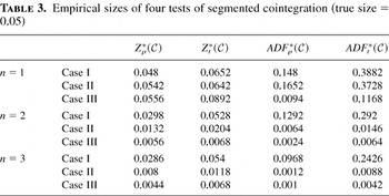
. Table 3 shows empirical sizes of the tests

at the 5% theoretical size. Overall, the Phillips–Perron–Ouliaris Z-tests show better size property than ADF tests. Since the values of test statistics are obtained from the segmentation of

,

whereas we use corresponding critical values for

, we expect that the tests would be conservative tests, having smaller actual sizes than the true size of 5%. This is evident for most cases of n = 2,3 for Z*.
Empirical sizes of four tests of segmented cointegration (true size = 0.05)

Next, we investigate the behavior of the tests under the alternative hypothesis H1, power properties of the tests. This is to evaluate the results of Lemma 2 by simulation. The simulation is based on samples of size 200 with 2,000 replications. We consider the following cointegration regression with an AR(1) error:

where

, β = 1, α = 0, and νt ∼ i.i.d.N(0,σ2) for σ2 = 0.1. We consider three different values of ρ, ρ = 0.85, 0.9, 0.95.
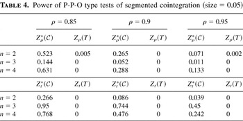
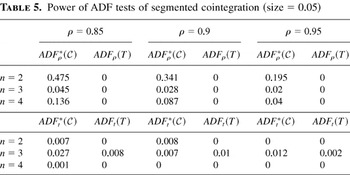
Tables 4 and 5 show power values of the tests

for testing H0 against H1 under three different values of ρ in H1 for the 5% test. Also, in Tables 4 and 5 we have power values of ordinary Z(T) and ADF(T) statistics where Z(T) and ADF(T), respectively, are the Z- and ADF-statistics obtained from the nonsegmented OLS based on the sample generated from the model (4.1). Power values of Z(T) and ADF(T) are very low for all the cases under study. This implies that the test obtained from the nonsegmented OLS tends to lead to the conclusion of noncointegration even if a cointegration relation prevails in 80% of the sample period, [0,1][setmn ][0.4,0.6] , an implication of Section 2.2. On the other hand, power values of

are quite high for all the cases under study, a result supporting the conclusion of Lemma 2.
Power of P-P-O type tests of segmented cointegration (size = 0.05)

Power of ADF tests of segmented cointegration (size = 0.05)

5. CONCLUSION
Many empirical works find that real data often fail to confirm cointegration for some well understood economic relations. Also, if a cointegration is confirmed by real data, the evidence is quite weak in many cases. We hope that this paper provides a probe to examine whether there indeed exists a cointegration relation except for some exceptional periods in the data. In Kim (2001) the Fisher relation is studied based on the procedure proposed in this paper. For U.S. postwar quarterly data, Kim (2001) finds that short-run nonstationary deviations in the data cause failure of the Fisher relation and that there exists a stable Fisher relation in the postwar era except for a period of several years. The Fisher relation is currently under study by the author of this paper much more in depth in the context of segmented cointegration and related inference methods.
APPENDIX: MATHEMATICAL PROOFS
Proof of Theorem 1. Except for the fact that we have segmentation with

the asymptotics in (3.8) and (3.9) are similar to the corresponding results of Phillips and Ouliaris (1990).
Proof of Theorem 2. The result is an immediate consequence of the continuous mapping theorem of Chan and Wei (1988) applied to the statistics

. █
Proof of Lemma 1. Let

be the volume of the set (i.e., the Lebesque measure)

. Then, it is true that

for [ell ]1 < [ell ]2. Therefore,

for every sample realization. Then, the conclusion of Lemma 1 follows.
Proof of Lemma 2. Except that they are obtained based on a regression for samples with segmentation the statistics

under H1 have the same properties as the corresponding statistics in Phillips (1987), Phillips and Perron (1988), and Phillips and Ouliaris (1990) under H1 of εt, t = 1,…,T, being I(0). This is particularly so for the magnitude of the statistics. Then, under the given conditions the conclusion of Lemma 3 immediately follows from Theorem 5.1 of Phillips and Ouliaris (1990). █
Proof of Theorem 3. (a) Since the same analysis is applicable for all (2.1a)–(2.1c), we consider the regression (2.1a). Let U(τ0) be an open neighborhood of τ0, the true value of τ, and

be a local base of τ0 containing all such neighborhoods. To prove that

it is sufficient to show that for each


for any η > 0. Notice that P[ΛT(τ0) > 0] = 1 and ΛT(τ0) = Op(1) since the numerator and the denominator of Λ(τ0) are of Op(1) with the probability limit of each being nonzero.
Let δ > 0 be an arbitrary number. To prove (A.1) it is sufficient to show that for τi = τi0 + ε or τi = τi0 − ε, i = 0,1, for 0 < ε < δ

uniformly in ε. Since the analysis is the same for i = 0 and for i = 1, we consider only the case of i = 0. For simplicity, fix τ1 = τ10. Consider first the case of τ0 = τ00 + ε. In this case (A.2) follows because the numerator of ΛT(τ) is of Op(1) whereas the denominator is of Op(κT) for a real number

, which is the result of the following: data in a portion of the noncointegration period, (τ00,τ0), are used for estimating

. Therefore, the estimator

is not consistent, and thus the residual process et is nonstationary for the whole data period in this case.
Now, consider the case τ0 = τ00 − ε for ε ∈ (0,δ). Notice that in this case

is consistently estimated. Hence, it follows that

uniformly in ε where

under the assumption that the noncointegration period is {τ00T + 1,…,τ10T}. Also notice that the dominant term in (A.3) is

But this dominant term is less than the numerator of ΛT(τ0):

since τ0 = τ00 − ε for ε > 0. Then, it follows that ΛT(τ) < ΛT(τ0) for τ0 = τ00 − ε uniformly in ε ∈ (0,δ). Notice that under Assumption 2 the denominator of (A.3) and that of ΛT(τ0) are asymptotically equivalent. This completes the proof. █
(b) Define UT(τ0,C) = {τ : |T(τ − τ0)| < C} for C > 0. It is sufficient to show that for all T > T0 for a sufficiently large T0 there exists a C such that C > 0 and

To prove (A.5) it is sufficient to show that there exists a finite real number C > 0 such that, for τ = (τ0,τ1) with τiT = τi0T + Mi or τiT = τi0T − Mi for Mi > C for i = 0,1,

uniformly in M = (M0,M1) for all T > T0 and for each η > 0. Since the analysis is the same for i = 0 and for i = 1, we consider only the case of i = 0. For simplicity, fix τ1 = τ10. Consider first the case of τ0T = τ00T + M0. In this case (A.6) follows because for a suitable choice of C the numerator of ΛT(τ) is of Op(1) whereas the denominator is of Op(κT) for a real number

, which results from the following: data in a portion of the noncointegration period, (τ00T,τ0T), are used for estimating

. Therefore, for a suitable choice of C the estimator

cannot be consistent, and thus the residual process et is nonstationary for the whole data period in this case.
Now, consider the case τ0T = τ00T − M0 for M0 > C. Notice that in this case

is consistently estimated. Then, it follows that

uniformly in M0 where

under the assumption that the noncointegration period is {τ00T + 1,…,τ10T}. Also notice that the dominant term in (A.7) is

But this dominant term is less than the numerator of ΛT(τ0):

since τ0T = τ00T − M0 for M0 > C. Then, it follows that ΛT(τ) < ΛT(τ0) for τ0T = τ00T − M0 uniformly in M0 > C. This completes the proof. █
References
REFERENCES
Bai, J.
(1997)
Estimating multiple breaks one at a time.
Econometric Theory
13,
315–352.Google Scholar
Bai, J.,
R. Lumsdaine, &
J. Stock
(1998)
Testing for and dating common breaks in multivariate time series.
Review of Economic Studies
65,
395–432.Google Scholar
Balke, N.S. &
T.B. Fomby
(1996)
Threshold cointegration.
International Economic Review
38,
627–645.Google Scholar
Banerjee, A.,
J.K. Dolado,
J.W. Galbraith, &
D.F. Hendry
(1993)
Cointegration, Error Correction, and the Econometric Analysis of
Non-Stationary Data.
Oxford:
Oxford University Press.
Chan, N.H. &
C.Z. Wei
(1988)
Limiting distributions of least squares estimates of unstable
autoregressive processes.
Annals of Statistics
15,
1050–1063.Google Scholar
Dickey, D.A. &
W.A. Fuller
(1979)
Distribution of the estimators for autoregressive time series with
a unit root.
Journal of the American Statistical Association
74,
427–431.Google Scholar
Engle, R.F. &
C.W.J. Granger
(1987)
Co-integration and error correction: Representation, estimation,
and testing.
Econometrica
55,
251–276.Google Scholar
Gregory, A.W. &
B.E. Hansen
(1996)
Residual based tests for cointegration in models with regime shifts.
Journal of Econometrics
70,
99–126.Google Scholar
Hansen, H. &
S. Johansen
(1993) Recursive Estimation in Cointegrated VAR Models. Manuscript, University of Copenhagen.
Hendry, D.G.
(1995)
Dynamic Econometrics.
Oxford:
Oxford University Press.
Kim, J.Y.
(2000)
Detection of change in persistence of a linear time series.
Journal of Econometrics
95,
97–116.Google Scholar
Kim, J.Y.
(2001) Inference on Segmented Cointegration and Reconsideration of the Fisher Relation. Discussion paper, Department of Economics, State University of New York at Albany.
Leybourne, S.J.,
B.P.M. McCabe, &
A.R. Tremayne
(1996)
Can economic time series be differenced to stationarity?
Journal of Business and Economic Statistics
14,
435–446.Google Scholar
MacKinnon, J.G.
(1991)
Critical values for cointegration tests. In
R.F. Engle and
C.W.J. Granger (eds.),
Long-Run Economic Relationships: Readings in Cointegration, pp.
267–276.
Oxford:
Oxford University Press.
McCabe, B.P.M. &
A.R. Tremayne
(1995)
Testing a time series for difference stationarity.
Annals of Statistics
23,
1015–1028.Google Scholar
Phillips, P.C.B.
(1986)
Understanding spurious regressions in econometrics.
Journal of Econometrics
33,
311–340.Google Scholar
Phillips, P.C.B.
(1987)
Time series regression with unit roots.
Econometrica
55,
277–302.Google Scholar
Phillips, P.C.B.
(1998) Econometric Analysis of Fisher's Equation. Cowles Foundation Discussion Paper 1180.
Phillips, P.C.B. &
S. Ouliaris
(1990)
Asymptotic properties of residual based tests for cointegration.
Econometrica
58,
165–193.Google Scholar
Phillips, P.C.B. &
P. Perron
(1988)
Testing for a unit root in time series regression.
Biometrika
75,
335–346.Google Scholar
Siklos, P.L. &
C.W.J. Granger
(1997)
Temporary cointegration with an application to interest rate parity.
Macroeconomic Dynamics
1,
640–657.Google Scholar
Stock, J.H. &
M.W. Watson
(1994) Evidence on Structural Instability in Macroeconomic Time Series Relations, NBER Technical working paper 164.
Asymptotic critical values of Zρ*(C) and ADFρ*(C)
Asymptotic critical values of Zt*(C) and ADFt*(C)
Empirical sizes of four tests of segmented cointegration (true size = 0.05)
Power of P-P-O type tests of segmented cointegration (size = 0.05)
Power of ADF tests of segmented cointegration (size = 0.05)
 You have
Access
- 12
- Cited by