


1. Introduction
In order to design robot control laws with superior performance, the knowledge of a reliable dynamic model is of paramount importance. Accurate dynamic models are essential for achieving high-performance control, enabling improved trajectory tracking and enhancing robot responsiveness and adaptability in tasks involving physical contact. This is particularly relevant in applications such as sensorless collision detection and reaction [Reference Haddadin, De Luca and Albu-Schäffer1], as well as in force regulation or for the implementation of impedance and admittance control strategies [Reference Magrini and De Luca2], where the control objectives rely directly on the dynamic interaction between the robot and its surroundings [Reference Siciliano, Villani, Oriolo and De Luca3]. Since many of the physical parameters involved in robot dynamics – such as inertial properties, joint friction, and motor characteristics – are difficult to measure directly or may vary over time due to wear or payload changes, dynamic parameter identification emerges as a fundamental tool. By estimating these parameters from experimental data, identification techniques allow for the refinement of dynamic models used in control design, ensuring that model-based strategies such as computed torque control, model predictive control, or observer-based control schemes remain robust and effective under real-world conditions.
Typically, manufacturers do not release information about the dynamic models of their manipulators, preventing the robotics community from employing a valuable tool for designing high-performance tailored control algorithms. To overcome this issue, identification procedures are widely adopted [Reference Siciliano, Villani, Oriolo and De Luca3–Reference Janot, Vandanjon and Gautier5]. Comprehensive overviews of modern strategies can be found in refs. [Reference Leboutet, Roux, Janot, Guadarrama-Olvera and Cheng6, Reference Qin, Yin, Yang and Zhang7]. Recent developments include quaternion-based parameter estimation [Reference Cheng, Bi and Yuan8], identification based on Lie-theory dynamic modeling [Reference Luo, Yuan, Hu, Du, Bao and Zhou9], sensitivity-driven identification for hybrid robots [Reference Luo, Xiao, Liu, Mingli, Zhao and Liu10], friction-aware iterative approaches for collaborative platforms [Reference Li, Wei, Liu, He, Liu, Zhang and Li11], and a neural-network method based on backpropagation [Reference Zhang, Li, Shi, Wang, Zhang, Zhang and Wu12].
All these methods rely on the linear dependence of the robot dynamic equations on a reduced set of dynamic coefficients
 $\boldsymbol{\pi} \in \mathbb{R}^r$
[Reference Gaz, Flacco and De Luca13], also known as base parameters [Reference Khalil and Dombre14], which are in general linear combinations of the standard dynamic parameters
 $\boldsymbol{p}$
of each rigid body composing the robot. More in detail, each robot link has one parameter specifying the mass, three specifying the position of the center of mass (CoM), and six for the symmetric inertia tensor. Thus, a robot with
 $n$
rigid links has a total of
 $10n$
dynamic parameters, or
 $\boldsymbol{p} \in \mathbb{R}^{10n}$
. Furthermore, a number of additional dynamic parameters may be considered for modeling dissipative effects at the joints (e.g., viscous or Coulomb friction) and for including the presence of motor inertias. Due to their physical nature, the dynamic parameters satisfy some natural inequalities or constraints (e.g., link masses are positive and inertia tensors are symmetric). In the context of identification, this has led to the use of constrained optimization techniques [Reference Khorshidi, Dawood, Nederkorn, Bennewitz and Khadiv15] for obtaining feasible values of these parameters.
In general, not all dynamic parameters can be directly identified. In fact, there are some link parameters that do not influence the dynamics of a given robot and, as such, are never identifiable through motion experiments. Knowledge of the exact value of these parameters is not relevant for motion control. Moreover, most of the times the remaining parameters are not isolated in the equations of motion but will appear only in linear combinations with other parameters to form the abovementioned dynamic coefficients in the model. As a result, the total number of dynamic coefficients
 $\boldsymbol{\pi}$
to be identified is typically much smaller than the original number of dynamic parameters
 $\boldsymbol{p}$
, or
 $r \ll 10n$
.
In many robotic problems, ranging from trajectory planning to motion control, the knowledge of the dynamic coefficients
 $\boldsymbol{\pi}$
is all that is needed. However, there are cases that require the retrieval of a complete set of feasible values for the dynamic parameters
 $\boldsymbol{p}$
. This happens at least in two situations where high efficiency in numerical computations is critical: when performing dynamic simulations via a CAD-based robotic simulator and when implementing torque-level control laws under hard real-time constraints. In fact, when the number
 $n$
of links becomes large, the Euler–Lagrange (EL) equations are typically replaced by the recursive Newton–Euler (NE) equations. However, these require in principle the knowledge of all dynamic parameters
 $\boldsymbol{p}$
of the links in the kinematic chain (not only of the dynamic coefficients
 $\boldsymbol{\pi}$
, as instead for EL), motivating the resort to physically feasible parameter retrieval methods, particularly in the context of collaborative robots [Reference Li, Wei, Liu, He, Liu, Zhang and Li11, Reference Petrone, Ferrentino and Chiacchio16] and in payload identification [Reference Xu, Fan, Fang, Zhu and Zhao17].
When starting from a set of dynamic coefficients
 $\boldsymbol{\pi}$
that can be identified through motion experiments, the determination of a corresponding set of dynamic parameters
 $\boldsymbol{p}$
is a nonlinear problem, which admits, in general, an infinite number of solutions. Only some of these solutions will be physically feasible (e.g., with positive link masses or with the elements of the link inertia tensors satisfying a triangle inequality), whereas there is indeed only one solution that corresponds to the real robot. However, any admissible set of dynamic parameters
 $\boldsymbol{p}$
, that is, a solution that successfully reconstructs the robot dynamic motion identified by the dynamic coefficients
 $\pi$
, should be considered as valid, despite the numerical values of the parameters are not the true ones.
In our previous work [Reference Gaz, Cognetti, Oliva, Giordano and De Luca18], we introduced a framework to extract a complete set of dynamic parameters by combining classical identification techniques [Reference Siciliano, Villani, Oriolo and De Luca3, Reference Hollerbach, Khalil, Gautier, Siciliano and Khatib4] with a global optimization routine for constrained problems. Available a priori information may be integrated as a set of constraints, even beyond the feasibility conditions coming from the physics. Thus, this framework is able to retrieve a set of dynamic parameters
 $\boldsymbol{p}$
that is both admissible and feasible. As a result, it can be used reliably also in NE routines or in CAD-based simulators. The obtained set of feasible parameters can be expanded with known payload parameters or, conversely, can be employed for estimating the additional parameters of a payload, using identification techniques that exploit their structural contributions [Reference Gaz and De Luca19] or are based on parameter difference [Reference Xu, Tuo, Fang, Chen, Fan, Shan and Zhao20].
In the last few years, a new class of manipulators, named cobots (i.e., collaborative robots), has been introduced in the industrial context. The intrinsic safety of cobots, due to their lightweight link structure as well as the use of compliant transmission/actuation assembly, such as harmonic drives or VSA, has been one of the reasons for their success, the other being the availability of sensorless model-based control laws that can react promptly to accidental collisions occurring anywhere along the robot structure and safely handle intentional physical human–robot interaction (HRI). Several works have addressed the problem of identifying the dynamics of cobots, such as the KUKA LWR 4+ [Reference Gaz, Flacco and De Luca21–Reference Kolyubin, Shiriaev and Jubien23] (and its industrial counterpart, the KUKA iiwa [Reference Stürz, Affolter and Smith24]), the Universal Robots UR10 [Reference Gaz, Magrini and De Luca25], the Kinova Jaco Arm [Reference Golluccio, Gillini, Marino and Antonelli26], and the Franka Emika Panda [Reference Gaz, Cognetti, Oliva, Giordano and De Luca18].
The aim of this paper is to collect and expand the algorithms proposed by the authors for dynamic identification and parameter retrieval (including payload) in a single integrated framework for collaborative robots, as well as to present and validate their use for enhancing trajectory tracking and for safe HRI control. The main original contributions of the paper and their relation with the state-of-the-art are summarized as follows:
-
• A unified formulation is presented for the dynamic model identification problem of robots with rigid or elastic joints, when the latter are equipped with joint torque sensors.
-
• We extend the preliminary results published in ref. [Reference Gaz, Flacco and De Luca21], by reporting a complete feasible set of dynamic parameters for the 7-dof KUKA LWR 4+, a popular lightweight robot widely adopted, especially in research contexts. For this, we take advantage of our Penalty-Based Parameter Retrieval algorithm (henceforth, PBPR) presented in ref. [Reference Gaz, Cognetti, Oliva, Giordano and De Luca18] for a different robot. It should be noted that the dynamic identification results on the KUKA LWR 4+ robot published so far [Reference Janot, Vandanjon and Gautier5, Reference Kolyubin, Shiriaev and Jubien23] do not provide such values, but only those of the dynamic coefficients (i.e., of combinations of dynamic parameters) appearing in the model. On the other hand, the set of dynamic parameters reported in ref. [Reference Stürz, Affolter and Smith24] refers to a different robot of the same manufacturer, namely, the KUKA iiwa.
-
• We present a comparison between our identified dynamic coefficients of the KUKA LWR 4+ and the corresponding values reported in ref. [Reference Jubien, Gautier and Janot22]. The dynamic coefficients in ref. [Reference Jubien, Gautier and Janot22] were found following the modified Denavit–Hartenberg (DH) convention [Reference Craig27], while we adopted the classical DH convention [Reference Siciliano, Villani, Oriolo and De Luca3], which is a more common choice for robot modeling and control. In any event, the proposed identification framework is independent of the specific kinematic parametrization and can be applied using either the classical or the modified DH convention.
-
• Another novel feature is the possible integration of the retrieved dynamic parameters within the CoppeliaSim simulator [28]. The original CAD model of the KUKA LWR 4+ robot implemented in this simulator was developed by the second author of this paper. It is based on a set of dynamic parameters obtained empirically, using rough information about the material composition and mass distribution of the robot links. Here, we take advantage of the identification of dynamic coefficients and the use of the PBPR algorithm to extract a set of dynamic parameters, which can be directly included in the CoppeliaSim model. Being physically feasible, our new set of dynamic parameters allows to generate in simulation the needed motion torques for inverse dynamics as well as internal wrenches (i.e., forces and moments) that are closer to those that would be obtained on the real robot.
-
• A nonlinear joint friction model has been added to the identification process, when this is performed in a reverse engineering way, that is, by taking advantage of the available KUKA Fast Research Interface (FRI). This separate estimation allows to better capture the experimental results on inverse dynamics and can be used for improving the control performance in trajectory tracking.
-
• A recursive algorithm is presented that generates online an additional torque to compensate for the missing control action when a perfectly rigid robot and direct torque control is being assumed. In fact, the KUKA LWR 4+ displays a non-negligible elasticity at the joints due to the use of harmonic drives. This effect is typically masked by the presence of a low-level joint torque controller (not accessible to the user) that transfers the desired commanded torque from the motor side to the link side of the elastic transmissions. The additional torque generated by our recursive algorithm reduces the nonideal behaviors of such a low-level control loop.
-
• Finally, the obtained dynamic modeling results are illustrated through collision detection and isolation experiments that use model-based residuals that monitor the generalized momentum of the robot [Reference Haddadin, De Luca and Albu-Schäffer1]. The sensitivity and performance obtained with such a sensorless method validate the obtained dynamic identification results.
The paper is organized as follows. Section 2 describes the main features of the collaborative robot under study, the KUKA LWR 4+, together with its control architecture. In Section 3, the dynamic modeling for rigid robots and for elastic joint robots is recalled, and the corresponding dynamic identification problems are formulated and discussed. Section 4 addresses the problem of estimating the extra dynamic parameters due to the presence of an unknown end-effector payload. In Section 5, we formulate the dynamic identification problem of the KUKA LWR 4+ robot through a reverse engineering approach, namely taking advantage of the signals available through the FRI. In Section 6, the experimental identification results are presented, obtained either by the reverse engineering approach or by means of the PBPR algorithm. In the first approach, a nonlinear joint friction model is also introduced and validated; in the second, the complete linearly parametrized model that includes the friction coefficients is considered. Section 7 reports a comparison between the KUKA LWR 4+ dynamic model identified in this paper and the model embedded in CoppeliaSim. Two control applications that use the identified dynamic model are illustrated in Section 8. The first shows the performance improvement that can be achieved on a trajectory tracking task when including correctly identified dynamic terms in the feedforward action; it includes also the additional torque command that helps in reproducing a desired user-commanded torque compensating for the low-level elastic joint torque loop present in the KUKA robot. The second application is a model-based (thus, sensorless) collision detection experiment, possibly in the presence of an unknown payload, in which our results outperform those provided by the manufacturer; moreover, the detection of a collision may be followed by a safe reaction strategy, again through a reflex control law based on the identified dynamic model. Finally, Section 9 summarizes our conclusions.
2. KUKA LWR 4+ robot
The KUKA LWR 4+ (or IV+) robot considered in this paper is a lightweight anthropomorphic manipulator with 7 rotational joints actuated by brushless motors. Its total mass is about 16 kg, with a rated payload of 7 kg (very high, if compared with its own mass). The robot is low powered, using less than 80 W; this makes it suitable to work with accumulators (useful, e.g., in mobile applications) and for safe HRI tasks (according to ISO/TS 15066). Links are connected to motors by means of in-line harmonic drives, which offer high reduction ratios (
 $160$
for all joints, except joint
 $5$
with
 $100$
) and eliminate backlash. On the other hand, harmonic drives introduce non-negligible elasticity in the motion transmission at the joint (with stiffness
 $K_i=10,000$
Nm/rad for
 $i=1,\ldots ,5$
, and
 $K_i=7500$
Nm/rad for
 $i=6,7$
). Each joint is equipped with a high-resolution encoder position sensor on the motor (input) side and with a Hall position sensor and a torque sensor on the link (output) side of the harmonic drive. This (actually, redundant) combination of measurements allows to drive the robot links with position, velocity, or torque commands through a suitable low-level feedback control loop.
Classical and modified DH parameters of the KUKA LWR 4+ robot.

Table I. Long description
A table comparing classical and modified DH parameters of the KUKA LWR 4+ robot. The table has 7 rows and 10 columns. The columns are labeled as Link, Classical DH with sub-columns ai, αi, di, θi, and Modified DH with sub-columns ai, αi, di, θi. The rows are labeled with numbers from 1 to 7. Each row contains values for the corresponding link’s parameters. Row 1: Link 1, Classical DH ai 0, αi π/2, di 0, θi q1, Modified DH ai 0, αi 0, di 0, θi q1. Row 2: Link 2, Classical DH ai 0, αi -π/2, di 0, θi q2, Modified DH ai 0, αi π/2, di 0, θi q2. Row 3: Link 3, Classical DH ai 0, αi -π/2, di L1, θi q3, Modified DH ai 0, αi -π/2, di L1, θi q3. Row 4: Link 4, Classical DH ai 0, αi π/2, di 0, θi q4, Modified DH ai 0, αi -π/2, di 0, θi q4. Row 5: Link 5, Classical DH ai 0, αi π/2, di L2, θi q5, Modified DH ai 0, αi π/2, di L2, θi q5. Row 6: Link 6, Classical DH ai 0, αi -π/2, di 0, θi q6, Modified DH ai 0, αi π/2, di 0, θi q6. Row 7: Link 7, Classical DH ai 0, αi 0, di 0, θi q7, Modified DH ai 0, αi -π/2, di 0, θi q7.
Classical [left] and modified [right] DH frames of the KUKA LWR 4+. All
 $x$
-axes point toward the viewer (frames are displaced sideways for better clarity). Note that the origins of the classical and modified DH frames coincide for this robot.

To describe the robot kinematics, it is necessary to choose reference frames that allow to specify the relative location of successive joint axes for the entire system. The most used approach is based on the classical DH convention, but other choices are possible. In particular, an interesting alternative is represented by the so-called modified DH convention, introduced first in ref. [Reference Barker29].
A benefit offered by the modified DH convention is in the implementation of the iterative numerical NE algorithm for solving the inverse dynamics problem. It has been shown that, although equivalent, the modified DH convention requires less computational steps and is thus faster than the classical DH convention for real-time control [Reference Bianco30]. In this respect, we have carried out a comparison for the KUKA LWR 4+ robot between the performance of a NE routine written according to the two different DH conventions. While confirming the above result, the difference in execution times was found negligible for our purposes.
Figure 1 shows the KUKA LWR 4+ robot in its zero configuration, together with the link frames chosen according to the classical and the modified DH convention. The main difference is that in the modified DH convention, and the link frame i has its
 $z_{i}$
-axis aligned with the axis of joint i. Table I reports the DH parameters corresponding to the two conventions. For the purpose of dynamic analysis, the origin of the base frame and of the end-effector frame, namely of frame
 $0$
and frame
 $7$
in the classical DH convention, has been chosen at the intersection between the first and the second joint axis and, respectively, coincident with the origin of the sixth link frame. In this way, only the two link lengths
 $d_3=L_1=0.4$
m and
 $d_5=L_2=0.39$
m are left as nonzero kinematic parameters. Finally, in Table II, we provide for each joint the rotation angle
 $\psi _i$
about the
 $x_i$
-axis needed to superpose the classical DH reference frames to the modified DH reference frames.
The robot is commanded by means of a control unit (the KR C2 module) and a software interface (the FRI [31, Reference Kröger32]). The control unit allows to read link positions
 $\boldsymbol{q}$
and elastic joint torques
 $\boldsymbol{\tau}_{J}$
at a maximum sampling rate of 1 msec. The link position
 $\boldsymbol{q}$
is typically evaluated from the measurements of motor position
 $\boldsymbol{\theta }$
and elastic joint torque
 $\boldsymbol{\tau}_{J}$
. At each control step, it also allows to get numerical values of the link inertia matrix
 $\boldsymbol{M}_{\textrm {num}}({\boldsymbol{q}})$
, of the gravity vector
 $\boldsymbol{g}_{\textrm {num}}({\boldsymbol{q}})$
, and of the robot Jacobian matrix
 $\boldsymbol{J}_{\textrm {num}}({\boldsymbol{q}})$
at the current configuration
 $\boldsymbol{q}$
(Figure 2). Through the FRI library, the user can give reference commands that specify a desired joint position
 ${\boldsymbol{q}}_{\textrm{d}}$
, velocity
 $\dot {\boldsymbol{q}}_{\textrm {d}}$
, or even a torque
 $\boldsymbol{\tau}_{\textrm {user}}$
for moving the robot links. The control unit, thanks to low-level full state feedback controllers, transforms the input in the appropriate link-level torque that realizes the desired user command
 $\boldsymbol{\tau}_{\textrm {user}}$
.
Angles representing the rotations about the
 $x_i$
-axis from the classical DH reference frames to the modified DH reference frames.

Table II. Long description
Table with columns labeled ‘Link i’ and numbered 1 to 7. The table lists angles in radians for rotations about the x-axis from classical to modified DH reference frames. The angles are as follows: -π/2 for link 1, π/2 for link 2, π/2 for link 3, -π/2 for link 4, -π/2 for link 5, π/2 for link 6, and 0 for link 7.
Signal flows from/to the KUKA LWR 4+ robot and the KR C2 controller, including the FRI (software interface to the user).

3. Dynamic model identification
3.1. Procedure for rigid robots
In this section, we recall the dynamic modeling of a general
 $n$
-dof robot. We consider an open chain of links
 $\ell _i$
,
 $i = 1, \ldots , n$
, with mass
 $m_i$
. Let
 \begin{equation} {}^i {\boldsymbol{r}}_{i,ci} = \left (\!\begin{array}{c} c_{ix}\\ c_{iy} \\ c_{iz} \end{array}\!\right ) \qquad {}^i \boldsymbol{I}_{\ell _i} = \left (\!\begin{array}{ccc} I_{ixx} & \quad I_{ixy} & \quad I_{ixz} \\ I_{ixy} & \quad I_{iyy} & \quad I_{iyz} \\ I_{ixz} & \quad I_{iyz} & \quad I_{izz} \\ \end{array}\!\right )\!, \end{equation}
be, respectively, the position of the CoM and the inertia tensor relative to the CoM of the
 $i$
-th link
 $\ell _i$
, both expressed in the frame attached to link
 $i$
. Thus,
 ${}^i {\boldsymbol{r}}_{i,ci}$
and
 ${}^i \boldsymbol{I}_{\ell _i}$
are both constant.
Once a set
 ${\boldsymbol{q}} \in \mathbb{R}^n$
of generalized coordinates is chosen, the equations of motion are obtained by applying the Lagrange formulation, which is algorithmic and independent to the coordinate frames of reference. This approach starts from the expressions of the potential and the kinetic energy of each link and each motor in terms of the generalized coordinates.
The potential energy of the robot
 $\mathcal{U}({\boldsymbol{q}})$
is
 \begin{equation} \mathcal{U} = \sum _{i=1}^n \mathcal{U}_{\ell _i} = - \sum _{i=1}^n m_i \boldsymbol{\gamma }^T {\boldsymbol{r}}_{0,ci}, \end{equation}
where
 $\boldsymbol{\gamma }=\boldsymbol{\gamma }(g_0)$
is the gravity vector expressed in the absolute reference frame (with the gravity acceleration
 $g_0 = 9.81$
m/s
 $^2$
) and
 ${\boldsymbol{r}}_{0,ci}$
is the absolute position of the center of mass of link
 $i$
obtained from
 ${}^i {\boldsymbol{r}}_{i,ci}$
by applying the homogeneous transformation matrices.
The kinetic energy of the robot
 $\mathcal{T}({\boldsymbol{q}}, \dot {\boldsymbol{q}})$
is the sum, for each link, of the translational and rotational kinetic energy:
 \begin{equation} \mathcal{T} = \sum _{i=1}^n \mathcal{T}_{\ell _i} = \frac {1}{2} \sum _{i=1}^n \left ( m_i {}^i \boldsymbol{v}_{ci}^T {}^i \boldsymbol{v}_{ci} + {}^i\boldsymbol{\omega }_i^T \, {}^i \boldsymbol{I}_{\ell _i} {}^i \boldsymbol{\omega }_i \right )\!, \end{equation}
where
 ${}^i \boldsymbol{v}_{ci}$
and
 ${}^i \boldsymbol{\omega }_i$
are, respectively, the linear and the angular velocity of link
 $i$
, both referred to and expressed in the local frame. The velocity
 ${}^i \boldsymbol{v}_{ci}$
can also be expressed in terms of the linear velocity
 ${}^i \boldsymbol{v}_i$
of the origin of frame
 $i$
as
 \begin{equation} {}^i \boldsymbol{v}_{ci} = {}^i \boldsymbol{v}_i + \boldsymbol{S} \left ({}^i \boldsymbol{\omega }_i \right ) {}^i {\boldsymbol{r}}_{i,ci} = {}^i \boldsymbol{v}_i + \boldsymbol{S}^{T\!} \left ({}^i {\boldsymbol{r}}_{i,ci} \right ) {}^i \boldsymbol{\omega }_i, \end{equation}
where
 $\boldsymbol{S}({\cdot})$
is the skew-symmetric operator representing the vector product. Finally, according to Steiner theorem, the inertia tensor relative to the CoM can also be computed with respect to the origin of frame
 $i$
, still expressed in the corresponding frame:
 \begin{equation} {}^i \boldsymbol{J}_{\ell _i} = \left (\begin{array}{c@{\quad}c@{\quad}c} J_{ixx} & J_{ixy} & J_{ixz} \\ J_{ixy} & J_{iyy} & J_{iyz} \\ J_{ixz} & J_{iyz} & J_{izz} \end{array}\right ) = {}^i \boldsymbol{I}_{\ell _i} + m_i \,\boldsymbol{S}^{T\!}\left ( {}^i {\boldsymbol{r}}_{i,ci}\right ) \boldsymbol{S} \left ({}^i {\boldsymbol{r}}_{i,ci}\right )\!, \end{equation}
where the second term on the right side considers the translation of the point with respect to which the inertia tensor is evaluated (from the center of mass to the origin of frame
 $i$
).
In conclusion, we can rewrite Eq. (3) as
 \begin{equation} \mathcal{T} = \frac {1}{2} \sum _{i=1}^n \left ( m_i \Vert {}^i \boldsymbol{v}_i \Vert ^2 + {}^i\boldsymbol{\omega }_i^T \, {}^i \boldsymbol{J}_{\ell _i} \, {}^i \boldsymbol{\omega }_i + 2 m_i \, {}^i {\boldsymbol{r}}_{i,ci}^T \left ( {}^i \boldsymbol{v}_i \times ,{}^i \boldsymbol{\omega }_i \right )\right )\!, \end{equation}
and, in compact form, the robot dynamics as
 \begin{equation} \boldsymbol{M}({\boldsymbol{q}})\, \ddot {\!\boldsymbol{q}} + \boldsymbol{c}({\boldsymbol{q}},\dot {\boldsymbol{q}}) + \boldsymbol{g}({\boldsymbol{q}}) = \boldsymbol{\tau}\!, \end{equation}
where the inertia matrix
 $\boldsymbol{M}({\boldsymbol{q}})$
and the gravity vector
 $\boldsymbol{g}({\boldsymbol{q}})$
are obtained by symbolic differentiation of the kinetic energy
 $\mathcal{T}$
and potential energy
 $\mathcal{U}$
as
 \begin{equation} \boldsymbol{M}({\boldsymbol{q}}) = \nabla _{\dot {\boldsymbol{q}}}^2 \mathcal{T}({\boldsymbol{q}},\dot {\boldsymbol{q}}) \in \mathbb{R}^{n\times n}, \;\; \boldsymbol{g}({\boldsymbol{q}}) = \nabla _{\boldsymbol{q}}\, \mathcal{U}({\boldsymbol{q}}) \in \mathbb{R}^n\!, \end{equation}
 $\boldsymbol{c}({\boldsymbol{q}},\dot {\boldsymbol{q}})$
contains the Coriolis and centrifugal terms, and
 $\boldsymbol{\tau} \in \mathbb{R}^n$
is the vector of actuation (motor) torques.
The Coriolis and centrifugal terms are quadratic in the velocity
 $\dot {\boldsymbol{q}}$
and can be efficiently obtained in a factorized form by analytic differentiation of the elements of
 $\boldsymbol{M}({\boldsymbol{q}})$
[Reference Siciliano, Villani, Oriolo and De Luca3] using the Christoffel’s symbols as
 \begin{equation} \boldsymbol{c}({\boldsymbol{q}},\dot {\boldsymbol{q}}) = \boldsymbol{C}({\boldsymbol{q}},\dot {\boldsymbol{q}}) \dot {\boldsymbol{q}}, \end{equation}
where the
 $i$
-th row
 $\boldsymbol{c}_i^T$
of the
 $\boldsymbol{C}$
matrix is given by
 \begin{equation} \boldsymbol{c}_i^T = \frac {1}{2} \, \dot {\boldsymbol{q}}^T \left ( \left ( \frac {\partial \boldsymbol{m}_i}{\partial {\boldsymbol{q}}} \right ) + \left ( \frac {\partial \boldsymbol{m}_i}{\partial {\boldsymbol{q}}} \right )^T - \frac {\partial \boldsymbol{M}}{\partial q_i} \right )\!, \end{equation}
being
 $\boldsymbol{m}_i$
the
 $i$
-th column of the inertia matrix
 $\boldsymbol{M}$
.
It is well known [Reference Siciliano, Villani, Oriolo and De Luca3] that by defining and collecting the (standard) dynamic parameters of all robot links in the three vectors
 $\boldsymbol{p}_1 \in \mathbb{R}^{n}$
,
 $\boldsymbol{p}_2 \in \mathbb{R}^{3n}$
, and
 $\boldsymbol{p}_3 \in \mathbb{R}^{6n}$
, with
 \begin{equation} \begin{array}{l} \boldsymbol{p}_1 = \left ( \begin{array}{ccc} m_1 & \ldots & m_n \end{array}\right )^T \!, \\[5pt] \boldsymbol{p}_2 = \left ( \begin{array}{ccccccc} m_1 c_{1x} & m_1c_{1y} & m_1c_{1z} & \,\ldots \, & m_nc_{nx} & m_nc_{ny} & m_nc_{nz} \end{array} \right )^T\!, \\[5pt] \boldsymbol{p}_3 = \left ( \begin{array}{ccc} \mathcal{J}_{1}^T & \, \ldots \, & \mathcal{J}_{n}^T \end{array} \right )^T \!, \end{array} \end{equation}
where
 \begin{equation} \mathcal{J}_i = \left ( \begin{array}{cccccc} J_{ixx} & J_{ixy} & J_{ixz} & J_{iyy} & J_{iyz} & J_{izz} \end{array} \right )^T\!, \end{equation}
the dynamic model (7) displays a linear dependence on the introduced vector of dynamic parameters
 $\boldsymbol{p} =(\, \boldsymbol{p}_1, \boldsymbol{p}_2, \boldsymbol{p}_3) \in \mathbb{R}^{10n}$
, that is,
 \begin{equation} \boldsymbol{Y}_{p}\!\left ({\boldsymbol{q}},\dot {\boldsymbol{q}},\, \ddot {\!\boldsymbol{q}}\right ) \boldsymbol{p} = \boldsymbol{\tau}\!, \end{equation}
with the
 $n \times 10n$
regressor matrix
 $\boldsymbol{Y}_{p}$
.
It should be noted, however, that many of the dynamic parameters defined in (11) may not actually appear in the model (7). In addition, some of the remaining parameters will appear only in linear combinations, inducing a linear dependence of the corresponding columns of the regressor matrix
 $\boldsymbol{Y}_{p}$
, for all functional values
 $({\boldsymbol{q}},\dot {\boldsymbol{q}},\, \ddot {\!\boldsymbol{q}})$
, that is, along any possible trajectory
 ${\boldsymbol{q}}(t)$
. Indeed, this limits the individual identifiability of such dynamical parameters and would also cause numerical issues in any experimental identification procedure. For this purpose, it is always possible to further rearrange (13) as
 \begin{equation} \boldsymbol{Y}\!\left ({\boldsymbol{q}},\dot {\boldsymbol{q}},\, \ddot {\!\boldsymbol{q}}\right )\,\boldsymbol{\pi}(\, \boldsymbol{p}) = \boldsymbol{\tau}\!. \end{equation}
Equation (14) is now linearly parametrized in terms of a vector
 $\boldsymbol{\pi} \in \mathbb{R}^r$
of dynamic coefficients multiplied by the
 $n \times r$
regressor matrix
 $\boldsymbol{Y}$
of known time-varying functions and can be used to identify the vector
 $\boldsymbol{\pi}$
of dynamic coefficients. Typically, the number
 $r$
of dynamic coefficients
 $\boldsymbol{\pi}$
will be much smaller than
 $10n$
, the original number of dynamic parameters. The set of dynamic coefficients is not unique, depending on how recombination of dynamic parameters is performed, but its minimum number is unique. As a matter of fact, only the set of dynamic coefficients
 $\boldsymbol{\pi}$
can be identified through robot motion experiments, as illustrated in the following. Note that the obtained results hold whatever reference frames are being used in the kinematic description of the robot, in particular also with the classical DH convention.
Assume a perfect knowledge of the kinematic parameters that appear in
 $\boldsymbol{Y}$
, that we know the torques
 $\boldsymbol{\tau}$
applied by the motors, and that reliable measurements of joint positions
 $\boldsymbol{q}$
are available. From the latter, joint velocities
 $\dot {\boldsymbol{q}}$
and accelerations
 $\, \ddot {\!\boldsymbol{q}}$
can be computed offline by numerical differentiation. In principle, we could move from (13) to (14) by analyzing the symbolic structure of the regressor matrix
 $\boldsymbol{Y}_p$
and recognizing a minimum set of columns that are functionally independent so to obtain
 $\boldsymbol{Y}$
in (14) and accordingly the combinations of parameters
 $\boldsymbol{p}$
. While deleting zero columns in
 $\boldsymbol{Y}_p$
(i.e., those corresponding to dynamic parameters that are not involved in robot motion) is quite straightforward, the remaining task becomes soon prohibitive when the number
 $n$
of degrees of freedom is large. Therefore, we will proceed numerically starting from the regressor
 $\boldsymbol{Y}_p$
.
Collect a large number
 $m$
of motor torque samples, as obtained from the commanded motor currents, and of link position samples from a sufficiently exciting robot motion, and perform offline the required numerical differentiation of the positions. For each retrieved sample
 $(\boldsymbol{\tau}_{k},{\boldsymbol{q}}_k,\dot {\boldsymbol{q}}_k,\, \ddot {\!\boldsymbol{q}}_k)$
, we have
 \begin{equation} \boldsymbol{Y}_{\boldsymbol{p},k\!}\left ({\boldsymbol{q}}_k,\dot {\boldsymbol{q}}_k,\, \ddot {\!\boldsymbol{q}}_k\right ) \boldsymbol{p} = \boldsymbol{\tau}_{k}, \qquad k = 1, \ldots , m, \end{equation}
so that we can stack these quantities in vectors and matrices as
 \begin{equation} \overline {\boldsymbol{Y}}_{p}\, \boldsymbol{p} = \overline {\boldsymbol{\tau}}, \end{equation}
with
 $\overline {\boldsymbol{\tau}} \in \mathbb{R}^{mn}$
and
 $\overline {\boldsymbol{Y}}_{p} \in \mathbb{R}^{mn \times 10n}$
.
In Eq. (16), the linearly dependent columns in the regressor should be grouped to obtain a full column rank matrix. The detection of linearly dependent columns in the stacked regressor matrix can be carried out numerically through the computation of its Reduced Row Echelon Form, obtained via a Gauss–Jordan elimination procedure. This allows to identify a maximal set of linearly independent columns and consequently determine the combinations of dynamic parameters that should be grouped in the vector of dynamic coefficients.
Following, for example, the procedure suggested in ref. [Reference Khalil and Dombre14], a generic parameter
 $p_j$
can be grouped with other parameters
 $p_{j1},\ldots ,p_{js}$
if the column
 $\boldsymbol{D}^{\, j}$
of the regressor
 $\overline {\boldsymbol{Y}}_{p}$
is linearly dependent on
 $\boldsymbol{D}^{\, j1}, \ldots , \boldsymbol{D}^{\, js}$
, or
 \begin{equation*} {\boldsymbol{D}}^{\, j} = t_{j1}{\boldsymbol{D}}^{\, j1} + \ldots + t_{js}{\boldsymbol{D}}^{\, js}, \end{equation*}
where
 $t_{jk}$
are constants, for
 $k=1,\ldots ,s$
. In this case, the column
 ${\boldsymbol{D}}^{\, j}$
and the dynamic parameter
 $p_j$
can be eliminated, while the parameters
 $p_{j1},\ldots ,p_{js}$
will be replaced by
 $p_{j1}^R,\ldots ,p_{js}^R$
, where
 $p_{jk}^R = p_{jk} + t_{jk}p_j$
, for
 $k=1,\ldots ,s$
.
Applying this pruning, redundant rows may appear in the modified dynamic parameter vector
 $\boldsymbol{p}^R$
after the replacements because a modified parameter happens to be a multiple of another (or of others) or vanishes. In that case, one should also prune the redundant rows and eliminate those that are actually dependent (or, in particular, zero). Let
 $p_i^R$
be a generic modified dynamic parameter. If
 \begin{equation} p_i^R = \lambda _{i1} p^R_{i1} + \ldots + \lambda _{il} p^R_{il}, \end{equation}
where
 $\lambda _{ih}$
are constants, for
 $h=1,\ldots ,l$
, then we eliminate the column
 $\boldsymbol{D}^i$
of the regressor as well as the coefficient
 $p_i^R$
, and replace the columns
 $\boldsymbol{D}_{i1},\ldots ,\boldsymbol{D}_{il}$
by
 $\boldsymbol{D}_{i1}^R,\ldots ,\boldsymbol{D}_{il}^R$
, where
 $\boldsymbol{D}_{ih}^R = \boldsymbol{D}_{ih} + \lambda _{ih}\boldsymbol{D}_i$
, for
 $h=1,\ldots ,l$
.
At the end of this procedure, the final pruned regressor matrix
 $\overline {\boldsymbol{Y}}_{p}^R$
, having
 $r \ll 10n$
columns (and still the same number
 $mn$
of rows), and the final modified vector of dynamic parameters
 $\boldsymbol{p}^R$
will continue to satisfy (16). As a result, we conclude that the obtained quantities are the same that would have been obtained by stacking the Eq. (14), and write
 \begin{equation*} \overline {\boldsymbol{Y}}_{p}^R \boldsymbol{p}^R = \overline {\boldsymbol{Y}}\, \boldsymbol{\pi}(\, \boldsymbol{p}) = \overline {\boldsymbol{\tau}}, \end{equation*}
where the final modified vector of dynamic parameters is baptized as the vector of dynamic coefficients
 $\boldsymbol{\pi} \in \mathbb{R}^r$
of the robot.
Therefore, choosing
 $m$
in (15) large enough (say, with
 $m n \gg 10 n$
), it is possible in this way to obtain a full column rank stacked regressor
 $\overline {\boldsymbol{Y}}$
and estimate the dynamic coefficients
 $\hat {\boldsymbol{\pi}}$
by solving a least squares problem via pseudoinversion
 \begin{equation} {\hat {\boldsymbol{\pi}}} = \overline {\boldsymbol{Y}}^{\,\#} \overline {\boldsymbol{\tau}} = \left ( \overline {\boldsymbol{Y}}^{\,T} \, \overline {\boldsymbol{Y}} \right )^{\!-1} \overline {\boldsymbol{Y}}^T \overline {\boldsymbol{\tau}}. \end{equation}
For validation purposes, the solution
 $\hat {\boldsymbol{\pi}}$
from (18) can be used to estimate the motor torques associated to a new robot motion, both in experiments and in numerical simulations, as
 \begin{equation} \hat {\boldsymbol{\tau}} = \boldsymbol{Y}\left ({\boldsymbol{q}},\dot {\boldsymbol{q}},\, \ddot {\!\boldsymbol{q}}\right ) {\hat {\boldsymbol{\pi}}}. \end{equation}
So far, we have not considered the presence of dissipative phenomena at the robot joints. However, it is straightforward to extend the previous formulation by including a decentralized joint friction model. In particular, for the
 $i$
-th joint, the friction torque can be modeled as
 \begin{equation} \tau _{fi}(\dot {q}_i)=f_{vi}\,\dot {q}_i +f_{ci}\,\mathrm{sign}(\dot {q}_i)+f_{oi}, \end{equation}
where
 $f_{vi} \ge 0$
and
 $f_{ci\ge 0}$
are the the viscous and Coulomb friction parameters, while the parameter
 $f_{oi}$
denotes an offset, that is, the friction torque present at
 $\dot q_i = 0$
. This model is decentralized because the friction acting at each joint depends only on the local joint velocity
 $\dot {q}_i$
. Moreover, since (20) is linear with respect to the three friction parameters and friction parameters do not recombine with any of the previous dynamic coefficients
 $\boldsymbol{\pi}$
, the introduced friction parameters are treated directly as additional dynamic coefficients within the identification procedure. More specifically, the vector of dynamic coefficients
 $\boldsymbol{\pi}$
is augmented by a set of
 $3n$
coefficients
 $\boldsymbol{\pi}_f$
, resulting in a total of
 $r_c = r+3n$
coefficients to be identified. Accordingly, the previously derived regressor matrix
 $\boldsymbol{Y}({\boldsymbol{q}},\dot {\boldsymbol{q}},\, \ddot {\!\boldsymbol{q}})$
is not altered but augmented with additional
 $3n$
columns
 $\boldsymbol{Y}_f(\dot {\boldsymbol{q}})$
associated to the friction terms. By construction,
 $\boldsymbol{Y}_f(\dot {\boldsymbol{q}})$
consists of three diagonal blocks. As a result, defining the friction torque vector
 \begin{equation*} \boldsymbol{\tau}_f(\dot {\boldsymbol{q}}) = \left (\!\begin{array}{ccc} \tau _{f1}(\dot {q}_1) & \ldots & \tau _{fn}(\dot {q}_n) \end{array} \right )^T, \end{equation*}
the complete robot dynamics becomes
 \begin{equation} \boldsymbol{M}({\boldsymbol{q}})\, \ddot {\!\boldsymbol{q}} + \boldsymbol{c}({\boldsymbol{q}}, \dot {\boldsymbol{q}}) + \boldsymbol{g}({\boldsymbol{q}}) = \boldsymbol{\tau} - \boldsymbol{\tau}_f(\dot {\boldsymbol{q}}), \end{equation}
and its linearly parametrized form is organized as
 \begin{equation} \boldsymbol{Y}_{c}({\boldsymbol{q}},\dot {\boldsymbol{q}},\, \ddot {\!\boldsymbol{q}})\, \boldsymbol{\pi}_{c} = \left (\begin{array}{cc} \boldsymbol{Y}({\boldsymbol{q}},\dot {\boldsymbol{q}},\, \ddot {\!\boldsymbol{q}}) \,&\, \boldsymbol{Y}_f(\dot {\boldsymbol{q}}) \end{array} \right ) \left (\begin{array}{c} \boldsymbol{\pi} \\ \boldsymbol{\pi}_f \end{array} \right ) = \boldsymbol{\tau}, \end{equation}
where the complete regressor
 $\boldsymbol{Y}_{\boldsymbol{c}}$
is a
 $n \times r_c$
matrix.
We note also that the previous pruning procedure for eliminating linearly dependent columns from the stacked regressor needs to be applied only to the original matrix
 $\overline {\boldsymbol{Y}}_p$
in Eq. (16), without considering friction. Stated differently, once the stacked regressor
 $\overline {\boldsymbol{Y}}$
has full column rank equal to
 $r$
, then the complete stacked regressor
 $\overline {\boldsymbol{Y}}_c$
will also have full column rank equal to
 $r_c=r+3n$
.
As a last dynamic modeling step, one should consider also the presence of the (electrical) motors in the robot structure. Each motor is an additional rigid body with its 10 dynamic parameters, as in (11). However, the mass of the motors can always be incorporated in the mass of the links. In particular, due to their positioning in the LWR 4+ open chain structure, the mass of the stator of the
 $i$
-th motor is added to the mass of link
 $i-1$
, while the mass of its rotor is added to the mass of link
 $i$
. Accordingly, the position of the CoM of each link will include also the motor presence. On the other hand, a standard assumption [Reference Siciliano, Villani, Oriolo and De Luca3] made for the kinetic energy of the motors is that the dominating effect for each motor is due to the inertia
 $J_{mi,zz}$
of the rotor around its spinning axis. This is particularly true when transmissions with a large reduction ratios
 $n_{ri}$
are used, since inertial coupling effects between the links and the rotors of the motors are then scaled down.
As a result, the robot dynamic model (21) will contain extra scalar acceleration terms of the form
 $(J_{mi,zz} n_{ri}^2) \,\ddot q_i = M_{mi} \ddot q_i$
for the
 $i$
-th motor, with
 $n_{ri} \gg 1$
. As such, also the motor parameters
 $M_{mi}$
, for
 $i=1,\ldots , n$
, will appear linearly in the model in a decentralized way and not recombined with any other term. Thus, the linear parametrization of the dynamic model can be further extended by including also the motor inertias so to contain a total of
 $r+4n$
dynamic coefficients.
However, this extension will not pursued further here. In fact, in the KUKA LWR 4+ robot as well as in other collaborative robots, the transmission between motors and links is achieved by means of harmonic drives with large reduction ratios (
 $100\,:\,1$
for joint 5 and
 $160\,:\,1$
for all the other six joints). These devices introduce elasticity at the joints and actually decouple the motor inertias from the dynamics of the links. This issue is further discussed more in general in the next section on robots with joint elasticity, where it will become apparent why the inclusion of motor inertias can be neglected in the identification problem when sensors of the elastic joint torques are available.
3.2. Unified formulation for robots with elastic joints
Flexibility in industrial robots is usually related to the intrinsic compliance of motion transmission/reduction elements, such as cables, belts, or harmonic drives. This is typically seen as a parasitic effect in conventional industrial robots, with elasticity being typically modeled as concentrated at the joints. On the other hand, in collaborative robots, joint elasticity is introduced intentionally in order to obtain passive mechanical compliance, which is more suited to safe physical human–robot interaction. This is also the case of the KUKA LWR 4+ robot.
Hereafter, we first describe briefly how it is possible to set up, under suitable assumptions, an identification procedure based on the standard dynamic model of robots with elastic joints (and rigid links), illustrating similarities and differences with respect to the fully rigid case. Then, we point out when and how the identification problem resumes to the one of the rigid case.
For dynamic modeling, two sets of generalized coordinates are introduced, one before and the other after the deflection of the joint, which is assumed to be in the linear domain of elasticity. Let
 $\boldsymbol{\theta } \in \mathbb{R}^n$
be the motor positions after the reduction ratios and
 ${\boldsymbol{q}} \in \mathbb{R}^n$
the link positions. In this way, the robot kinematic equations are functions of link variables only. Under the standard modeling assumptions introduced by Spong [Reference Spong33], the dynamic equations take the form
 \begin{eqnarray} \boldsymbol{M}({\boldsymbol{q}})\, \ddot {\!\boldsymbol{q}} + \boldsymbol{c}({\boldsymbol{q}}, \dot {\boldsymbol{q}}) + \boldsymbol{g}({\boldsymbol{q}}) &=& \boldsymbol{K}(\boldsymbol{\theta }-{\boldsymbol{q}}) - \boldsymbol{\tau}_{f \kern-0.4pt l} \end{eqnarray}
 \begin{eqnarray} \boldsymbol{M}_m \, \ddot {\!\boldsymbol{\theta }} + \boldsymbol{K}(\boldsymbol{\theta }-{\boldsymbol{q}}) &=& \boldsymbol{\tau} - \boldsymbol{\tau}_{fm}, \end{eqnarray}
where
 $\boldsymbol{M}$
,
 $\boldsymbol{c}$
, and
 $\boldsymbol{g}$
are the same terms defined in (7) for rigid robots,
 $\boldsymbol{M}_m = \mbox{diag}\left \{M_{m1}, \ldots , M_{mn}\right \}$
is the diagonal, positive definite matrix of motor inertias (reflected through the gear ratios),
 $\boldsymbol{K} = \mbox{diag}\left \{K_1,\ldots ,K_n\right \}$
is the diagonal, positive definite matrix of joint stiffness,
 $\boldsymbol{\tau} \in \mathbb{R}^n$
is the motor torque, and
 $\boldsymbol{\tau}_{f \kern-0.4pt l}$
and
 $\boldsymbol{\tau}_{fm}$
are dissipative torques, acting, respectively, on the link and on the motor side of the transmissions. Usually, friction at the motor side is much higher than friction at the link side. In particular, in the KUKA LWR 4+ robot,
 $\boldsymbol{\tau}_{fm}$
is compensated by the low-level controller in the KRC2 hardware, which implements a model-free compensation algorithm on the basis of a residual signal [Reference Tien, Albu-Schäffer, De Luca and Hirzinger34]. The
 $n$
-dimensional second-order differential Eqs. (23) and (24) are called the link and the motor equations. The link and motor equations are coupled through the elastic joint torque (also called link-level torque)
 \begin{equation} \boldsymbol{\tau}_{J} = \boldsymbol{K} \left (\boldsymbol{\theta } - {\boldsymbol{q}}\right )\!, \end{equation}
which is often directly measurable by joint torque sensors (as in the KUKA LWR 4+ and in other collaborative robots).
It can be easily shown [Reference Miranda-Colorado and Moreno-Valenzuela35, Reference Zollo, Lopez, Spedaliere, Aracil and Guglielmelli36] that the complete dynamic model (23)–(24) satisfies a linear parametrization property similar to the case of rigid robots – compare with Eq. (14). In fact, neglecting for the moment the dissipative terms, we can write
 \begin{align} \left (\begin{array}{ccc} \boldsymbol{Y}({\boldsymbol{q}},\dot {\boldsymbol{q}},\, \ddot {\!\boldsymbol{q}}) \,&\, \boldsymbol{O}_{n \times n} \,&\, \mbox{diag}\left \{q_1-\theta _1,\ldots , q_n - \theta _n\right \} \\[4pt] \boldsymbol{O}_{n \times n} \,&\, \mbox{diag}\left \{\ddot \theta _1, \ldots , \ddot \theta _n\right \} \,&\, \mbox{diag}\left \{\theta _1-q_1,\ldots , \theta _n-q_n\right \} \end{array}\right ) \left (\begin{array}{c} \boldsymbol{\pi} \\[3pt] \left (\begin{array}{c} M_{m1} \\ \vdots \\ M_{mn}\end{array}\right ) \\[20pt] \left (\begin{array}{c} K_1 \\ \vdots \\ K_n\end{array}\right ) \end{array}\right ) = \left (\begin{array}{c} \boldsymbol{0} \\ \boldsymbol{\tau} \end{array}\right )\!, \end{align}
or
 \begin{equation} \boldsymbol{Y}_{EJ}\left ({\boldsymbol{q}}, \boldsymbol{\theta }, \dot {\boldsymbol{q}}, \, \ddot {\!\boldsymbol{q}}, \, \ddot {\!\boldsymbol{\theta }}\right ) \boldsymbol{\pi}_{EJ} = \left (\begin{array}{c} \boldsymbol{0} \\ \boldsymbol{\tau} \end{array}\right )\!, \end{equation}
with
 $\boldsymbol{\pi}_{EJ} \in \mathbb{R}^{r+2n}$
, which is the property we were looking for. A similar situation holds in the presence of a linear parametrized model for the dissipative terms
 $\boldsymbol{\tau}_{f \kern-0.4pt l}$
and
 $\boldsymbol{\tau}_{fm}$
. In order to perform identification of the extended set of dynamic coefficients
 $\boldsymbol{\pi} \in \mathbb{R}^r$
(the same as in the rigid case), and of the elements of the diagonal matrices
 $\boldsymbol{M}$
and
 $\boldsymbol{K}$
(
 $2n$
more dynamic coefficients), one needs to have at least measurements of
 $\boldsymbol{\theta }$
and
 $\boldsymbol{q}$
available, performing then offline numerical differentiation to obtain
 $\dot {\boldsymbol{q}}$
,
 $\ddot {\!\boldsymbol{q}}$
and
 $\ddot {\!\boldsymbol{\theta }}$
. Note that measurements of motor position
 $\boldsymbol{\theta }$
and of elastic joint torque
 $\boldsymbol{\tau}_{J}$
may also work, using the additional knowledge of
 $\boldsymbol{K}$
to obtain the needed
 $\boldsymbol{q}$
from (25).
An interesting alternative is available when only a measure of the link position
 $\boldsymbol{q}$
is available. Following the scheme of feedback linearization control, see, for example, Chapter 11 in [Reference Siciliano, Villani, Oriolo and De Luca3], Eqs. (23) and (24) can be rearranged eliminating the dependence from motor variables
 $\boldsymbol{\theta }$
. Differentiating twice in time the link equations and using the motor equations to substitute for
 $\, \ddot {\!\boldsymbol{\theta }}$
, one obtains after some manipulation (and dropping dependencies)
 \begin{equation} \boldsymbol{M}_m \boldsymbol{K}^{-1} \! \left ( \boldsymbol{M} \, {\stackrel {\boldsymbol{\ldots .}}{\boldsymbol{q}}} + 2 \dot {\boldsymbol{M}}\, {\stackrel {\boldsymbol{\ldots }}{\boldsymbol{q}}} + \, \ddot {\!\boldsymbol{M}} \, \ddot {\!\boldsymbol{q}} + \, \ddot {\!\boldsymbol{n}} \right ) + \left ( \boldsymbol{M} + \boldsymbol{M}_m \right ) \, \ddot {\!\boldsymbol{q}} + \boldsymbol{n} + \boldsymbol{\tau}_{f \kern-0.4pt l} + \boldsymbol{\tau}_{fm} + \boldsymbol{M}_m \boldsymbol{K}^{-1} \, \ddot {\!\boldsymbol{\tau}}_{f \kern-0.4pt l} = \boldsymbol{\tau}, \end{equation}
where
 $\boldsymbol{n}=\boldsymbol{n}({\boldsymbol{q}}, \dot {\boldsymbol{q}}) = \boldsymbol{c}({\boldsymbol{q}}, \dot {\boldsymbol{q}}) + \boldsymbol{g}({\boldsymbol{q}})$
for compactness. Neglecting dissipative terms as before for simplicity, (28) can be written in the compact, linearly parametrized form
 \begin{equation} \tilde {\boldsymbol{Y}}_{EJ}\left ({\boldsymbol{q}} , \dot {\boldsymbol{q}} , \, \ddot {\!\boldsymbol{q}}, {\stackrel {\boldsymbol{\ldots }}{\boldsymbol{q}}}, {\stackrel {\boldsymbol{\ldots .}}{\boldsymbol{q}}}\right ) \tilde {\boldsymbol{\pi}}_{EJ} = \boldsymbol{\tau}, \end{equation}
i.e., in terms of a set of extended dynamic coefficients
 $\tilde {\boldsymbol{\pi}}_{EJ} \in \mathbb{R}^{r(n+1)}$
and of a regressor matrix
 $\tilde {\boldsymbol{Y}}_{EJ}$
that depends only on link position and its derivatives up to the fourth order. Using Eq. (29), one can proceed in principle to dynamic identification as in the rigid case (with multiple offline differentiation of the position measurements).
At this stage, we note that, apart from the more complex regressor matrices or the larger number of numerical differentiations needed for the measured positions, one should have access for identification purposes to the motor torque
 $\boldsymbol{\tau}$
that is actually being applied to the robot. In the case of the KUKA LWR 4+ robot, this information is not directly available. On the other hand, measurement of the elastic joint torque
 $\boldsymbol{\tau}_{J}$
is provided by the joint torque sensors, together with a measure of the motor position
 $\boldsymbol{\theta }$
and knowledge of the joint stiffness
 $\boldsymbol{K}$
. Thus, the link position
 $\boldsymbol{q}$
can be obtained from (25) as
 \begin{equation} {\boldsymbol{q}} = \boldsymbol{\theta } - \boldsymbol{K}^{-1} \boldsymbol{\tau}_{J}. \end{equation}
As a result, dynamic identification of the KUKA LWR 4+ robot can be performed directly using the link Eq. (23) only, where the measured elastic joint torque
 $\boldsymbol{\tau}_{J}$
replaces the commanded motor torque
 $\boldsymbol{\tau}$
of the rigid case in the right-hand side of (14). Neglecting for the time being the (usually, small) friction terms acting on the link side of the elastic transmission, Eq. (14) is simply replaced by
 \begin{equation} \boldsymbol{Y}\! \left ({\boldsymbol{q}}, \dot {\boldsymbol{q}}, \, \ddot {\!\boldsymbol{q}}\right ) \boldsymbol{\pi}(\, \boldsymbol{p}) = \boldsymbol{\tau}_{J}. \end{equation}
As for the friction torque
 $\boldsymbol{\tau}_{f \kern-0.4pt l}$
acting on the link side, we can reintroduce and identify separately this term using also a nonlinear model, as it will be shown in Section 6.3. Or we can use a linear parametrization for these dissipative terms as in (22) and pursue then a complete identification approach using
 \begin{equation} \boldsymbol{Y}_{c}({\boldsymbol{q}},\dot {\boldsymbol{q}},\, \ddot {\!\boldsymbol{q}})\, \boldsymbol{\pi}_{c} = \boldsymbol{\tau}_{J}, \end{equation}
as it will be shown in Section 6.4.
4. Modified dynamic coefficients due to a payload
We briefly recall the problem of estimating the effect on the original robot dynamic coefficients of an extra unknown payload rigidly attached to the end effector. The problem has been addressed in ref. [Reference Gaz and De Luca19], where we proposed a model-based approach using two sets of experimental data, first without and then with the payload. As shown in ref. [Reference Gaz and De Luca19], the original set of dynamic coefficients changes when a payload is added, but the property of linearity of the parametrized dynamic equations is preserved and is independent from the specific choice of kinematic reference frames.
Let
 $m_L$
be the mass of the payload,
 ${}^n{\boldsymbol{r}}_{n,cL} = (\begin{array}{ccc} c_{Lx} & c_{Ly} & c_{Lz} \end{array} )^T$
the position of its CoM with respect to the origin of last robot frame
 $n$
, and
 ${}^n\boldsymbol{J}_L$
its symmetric inertia tensor relative to the last frame
 $n$
. The dynamic parameters of the payload can be organized in a vector
 \begin{equation} \boldsymbol{p}_L = ( \begin{array}{ccccc} m_L & m_L c_{Lx} & m_Lc_{Ly} & m_L c_{Lz} & \mathcal{J}_L \end{array} )^T \in \mathbb{R}^{10}, \end{equation}
where
 $\mathcal{J}_L \in \mathbb{R}^6$
is defined similarly to (12) using the symmetry of the inertia tensor.
The problem is to identify the new set
 $\boldsymbol{\pi}_L=\boldsymbol{\pi}_L(\, \boldsymbol{p},\boldsymbol{p}_L)$
of robot dynamic coefficients in the presence of a payload. We assume that a reliable estimate
 $\hat {\boldsymbol{\pi}}$
of the robot dynamic coefficients is available in the absence of the payload. Moreover, neglect for ease of presentation any dissipative effect. Define the symbolic difference vector
 \begin{equation} \boldsymbol{\varepsilon }(\, \boldsymbol{p}_L) = \boldsymbol{\pi}_L(\, \boldsymbol{p},\boldsymbol{p}_L) - \boldsymbol{\pi}(\, \boldsymbol{p}), \end{equation}
where the symbolic expression of the dynamic coefficient vector
 $\boldsymbol{\pi}_L$
is obtained from
 $\boldsymbol{\pi}(\, \boldsymbol{p})$
by applying the following linear mapping:
 \begin{equation} \begin{array}{l} m_{n} \,\rightarrow \, m_{n}+m_{L} \\[2pt] \! \begin{array}{l} m_{n} c_{nx} \, \rightarrow \, m_{n} c_{nx} + m_{L} c_{Lx} \\ m_{n} c_{ny} \, \rightarrow \, m_{n} c_{ny} + m_{L} c_{Ly} \\ m_{n} c_{nz} \, \rightarrow \, m_{n} c_{nz} + m_{L} c_{Lz} \end{array} \\[15pt] {}^n\boldsymbol{J}_{n} \,\rightarrow \, {}^n\boldsymbol{J}_{n}+\, {}^n\boldsymbol{J}_{L}= \left (\begin{array}{ccc} J_{nxx}+J_{Lxx} \,&\, J_{nxy}+J_{Lxy} \,&\, J_{nxz}+J_{Lxz} \\ J_{nxy}+J_{Lxy} \,&\, J_{nyy}+J_{Lyy} \,&\, J_{nyz}+J_{Lyz} \\ J_{nxz}+J_{Lxz} \,&\, J_{nyz}+J_{Lyz} \,&\, J_{nzz}+J_{Lzz} \end{array}\right )\!. \end{array} \end{equation}
Thanks to (34), we can write the dynamics of the loaded robot as
 \begin{equation} \boldsymbol{Y}_L({\boldsymbol{q}},\dot {\boldsymbol{q}},\, \ddot {\!\boldsymbol{q}})\,\boldsymbol{\pi}(\, \boldsymbol{p}) + \boldsymbol{Y}_L({\boldsymbol{q}},\dot {\boldsymbol{q}},\, \ddot {\!\boldsymbol{q}})\,\boldsymbol{\varepsilon }(\, \boldsymbol{p}_L) = \boldsymbol{\tau} _L, \end{equation}
where
 $\boldsymbol{Y}_L({\boldsymbol{q}},\dot {\boldsymbol{q}},\, \ddot {\!\boldsymbol{q}}) = \boldsymbol{Y}({\boldsymbol{q}},\dot {\boldsymbol{q}},\, \ddot {\!\boldsymbol{q}})$
is the same regressor matrix of the unloaded case (after pruning), evaluated under the action of the torque
 $\boldsymbol{\tau}_L$
(or, in view of the analysis of Section 3.2, of
 $\boldsymbol{\tau}_{J,L}$
) in the presence of the payload.
The identification procedure for the modified robot coefficients
 $\boldsymbol{\pi}_L$
is the same as for the unloaded case, with the only difference that it takes advantage of the previously estimated dynamic coefficients
 $\hat {\boldsymbol{\pi}}$
. The robot will execute a set of sufficiently exciting [Reference Rackl, Lampariello and Hirzinger37] trajectories, which may be the same or differ from those of the unloaded case. We collect the joint torques
 $\overline {\boldsymbol{\tau}}_L$
and the motion data, process them, and organize a linear set of equations as
 \begin{equation} \overline {\boldsymbol{Y}}_L \,\boldsymbol{\pi}_L = \overline {\boldsymbol{\tau}}_L, \end{equation}
where
 $\overline {\boldsymbol{Y}}_L$
is the stacked regressor evaluated with the performed experiments. Then, the estimated coefficients of the loaded case are computed again by pseudoinversion as
 \begin{equation} {\hat {\boldsymbol{\pi}}}_L = \overline {\boldsymbol{Y}}_L^\# \, \overline {\boldsymbol{\tau}}_L. \end{equation}
Using (34), we also obtain the numerical difference vector
 $\hat {\boldsymbol{\varepsilon }}$
as
 \begin{equation} \hat {\boldsymbol{\varepsilon }} = {\hat {\boldsymbol{\pi}}}_L - {\hat {\boldsymbol{\pi}}}. \end{equation}
Note that in practice the estimation of
 ${\hat {\boldsymbol{\pi}}}_L$
and
 $\hat {\boldsymbol{\pi}}$
will not change when using a different or just the same sufficiently exciting trajectory in the two experiments. When the trajectory for the unloaded and the loaded robot is the same, one has
 $\overline {\boldsymbol{Y}} = \overline {\boldsymbol{Y}}_L$
and can compute then
 $\hat {\boldsymbol{\varepsilon }}$
equivalently as
 \begin{equation} \hat {\boldsymbol{\varepsilon }} = \overline {\boldsymbol{Y}}^{\#} \left ( \overline {\boldsymbol{\tau}}_L - \overline {\boldsymbol{\tau}}\right )\!. \end{equation}
The above analysis and the resulting value of vector
 $\hat {\boldsymbol{\varepsilon }}$
allows to obtain also an estimate for the 10 dynamic parameters
 $\boldsymbol{p}_l$
of the payload in (33). Defining the payload Jacobian
 $\boldsymbol{J}_{\boldsymbol{\varepsilon }}$
as the matrix of symbolic partial derivatives of
 $\boldsymbol{\varepsilon }(\, \boldsymbol{p}_L)$
with respect to vector
 $\boldsymbol{p}_L$
, we have
 \begin{equation} \boldsymbol{J}_{\boldsymbol{\varepsilon }} = \frac {\partial \boldsymbol{\varepsilon }(\, \boldsymbol{p}_L) }{\partial \boldsymbol{p}_L} \quad \Rightarrow \quad \boldsymbol{J}_{\boldsymbol{\varepsilon }}\boldsymbol{p}_L = \boldsymbol{\varepsilon }, \end{equation}
thanks to the linearity of (35). Therefore, the payload parameters can be estimated as
 \begin{equation} \hat {\boldsymbol{p}}_L = \boldsymbol{J}_{\boldsymbol{\varepsilon }}^{\#}\hat {\boldsymbol{\varepsilon }}. \end{equation}
The accuracy of such an estimation typically increases with the number
 $r$
of dynamic coefficients of the given robot, and thus implicitly with the number
 $n$
of its degrees of freedom.
5. Dynamic identification via a reverse engineering approach
As mentioned in Section 2, the FRI software interface and the controller of the KUKA LWR 4+ manipulator allow to perform the identification of all dynamic coefficients
 $\boldsymbol{\pi}$
that are present in the left-hand side of the model (31) using only data collected at a sufficiently large set of robot configurations, without the need to resort to numerical reconstruction of velocities and accelerations.
In fact, the FRI software provides the numerical values
 $\boldsymbol{g}_{\textrm {num}}({\boldsymbol{q}})$
and
 $\boldsymbol{M}_{\textrm {num}}({\boldsymbol{q}})$
of the components of the robot gravitational vector
 $\boldsymbol{g}({\boldsymbol{q}})$
and, respectively, of the elements of the robot inertia matrix
 $\boldsymbol{M}({\boldsymbol{q}})$
at any current configuration
 $\boldsymbol{q}$
. Thus, a large amount of data can be acquired in a static way, avoiding the necessity to execute exciting trajectories for the robot. Once the robot is brought to a desired configuration, the numerical values of joint position, gravity vector, and inertia matrix are read and stored. Accordingly, one can also read and store the elastic joint torque
 $\boldsymbol{\tau}_{J}$
measured in the same configurations. These measurements are not needed in this identification approach, but are used later for validation purposes. Note that the procedure is not influenced by friction nor by any other dynamic effects not considered in the dynamic model.
Since the numerical information provided is based on an internal dynamic model used by the robot manufacturer and their engineers, this model is assumed to be sufficiently reliable for extracting the actual dynamic coefficients of the robot. For this reason, we called this a reverse engineering approach to dynamic identification. In a similar way, the approach described below can be applied also to other robots that return the same data as the KUKA LWR 4+, for example, the Franka Emika Research 3 manipulator.
The starting point is that the linear parametrization of the whole model discussed in Section 3 holds also for the single terms in the dynamic equations. The coefficients related to link masses and to positions of the link centers of mass can be factored out from the gravity vector
 $\boldsymbol{g}({\boldsymbol{q}})$
. In particular, by exploiting the linearity property and the fact that the LWR 4+ robot has only revolute joints, this can be done by collecting and reorganizing all possible individual trigonometric functions (or products of functions) present in the gradient of the symbolic expression of the potential energy. As a result, the gravity term in the model can be written as
 \begin{equation} \boldsymbol{g}({\boldsymbol{q}}) = \boldsymbol{Y}_g({\boldsymbol{q}})\,\boldsymbol{\pi}_g. \end{equation}
with a vector of gravity-related dynamic coefficients
 $\boldsymbol{\pi}_g \in \mathbb{R}^{r_g}$
to be estimated. In doing so, we assume knowledge of the gravity acceleration
 $g_0$
, which will be included in the (known) symbolic expression of the
 $n \times r_g$
regressor matrix
 $\boldsymbol{Y}_g$
.
The elements of the robot inertia matrix
 $\boldsymbol{M}({\boldsymbol{q}})$
can be retrieved from a similar linear factorization. First, we rearrange the lower-triangular elements
 $M_{ij}({\boldsymbol{q}})$
, with
 $i=1,\ldots , n$
and
 $j=1, \ldots , i$
, of this symmetric matrix in vector form, so to obtain a vector
 $\boldsymbol{m}({\boldsymbol{q}}) \in \mathbb{R}^{n(n+1)/2}$
. For the considered robot with
 $n=7$
joints, this vectorization gives
 \begin{equation*} \boldsymbol{m}({\boldsymbol{q}}) = (\begin{array}{cccccccccccccccc} M_{11} & M_{21} & M_{22} & M_{31} & \ldots & M_{33} & M_{41} & \ldots & M_{44} & \, \ldots \, & M_{61} & \ldots & M_{66} & M_{71} & \ldots & M_{77} \end{array} )^T \in \mathbb{R}^{28}. \end{equation*}
Proceeding as before by collecting and reorganizing all trigonometric functions present in the hessian of the symbolic expression of the kinetic energy, we can write
 \begin{equation} \boldsymbol{m}({\boldsymbol{q}}) = \boldsymbol{Y}_m({\boldsymbol{q}})\,\boldsymbol{\pi}_m, \end{equation}
with a vector of inertia-related dynamic coefficients
 $\boldsymbol{\pi}_m \in \mathbb{R}^{r_m}$
to be estimated and a corresponding
 $n \times r_m$
regressor matrix
 $\boldsymbol{Y}_m$
. Vector
 $\boldsymbol{\pi}_m$
contains in general linear combinations of all link parameters
 $\boldsymbol{p} \in \mathbb{R}^{10n}$
, that is, their masses, the positions of their centers of mass, as well as the elements of their inertia tensors. We also note that, in this approach, the required separate treatment of the gravity vector and of the (stacked) inertia matrix gives rise to a number of dynamic coefficients
 $r_g+r_m$
, which may be (and typically is) larger than the minimum number
 $r$
that is obtained when following the classical procedure presented in Section 3.1 for the dynamic model as a whole.
The identification experiment consists in collecting FRI data and measurements in a sufficiently large number
 $m$
of different configurations. For a generic configuration
 ${\boldsymbol{q}}_k$
,
 $k = 1, \ldots , m$
, we can write
 \begin{equation} \boldsymbol{Y}_{g,k}({\boldsymbol{q}}_k) \, \boldsymbol{\pi}_g = \ \boldsymbol{g}_{\textrm {num},k} \qquad \quad \boldsymbol{Y}_{m,k}({\boldsymbol{q}}_k) \, \boldsymbol{\pi}_m = \ \boldsymbol{m}_{\textrm {num},k}, \end{equation}
where the numerical terms on the right-hand sides are both retrieved from the FRI (vectorizing
 $\boldsymbol{M}_{\textrm {num}}$
to
 $\boldsymbol{m}_{\textrm {num}}$
, like it was done with
 $\boldsymbol{M}({\boldsymbol{q}})$
). Then, we stack these equations as
 \begin{equation} \overline {\boldsymbol{Y}}_g \boldsymbol{\pi}_g = \ \overline {\boldsymbol{g}}_{\textrm {num}} \qquad \quad \overline {\boldsymbol{Y}}_m \boldsymbol{\pi}_m = \ \overline {\boldsymbol{m}}_{\textrm {num}}. \end{equation}
For the
 $n=7$
joints of the KUKA LWR 4+ robot, the regressor matrices
 $\overline {\boldsymbol{Y}}_g$
and
 $\overline {\boldsymbol{Y}}_m$
are, respectively, of dimensions
 $7m \times r_g$
and
 $28m \times r_m$
. Accordingly,
 $\overline {\boldsymbol{g}}_{\textrm {num}} \in \mathbb{R}^{7m}$
and
 $\overline {\boldsymbol{m}}_{\textrm {num}} \in \mathbb{R}^{28m}$
.
Under the condition that
 $m \gg r_g + r_m$
, if both regressors have full column rank, the two overconstrained linear equations in (46) can be solved in a least squares sense by using the pseudoinverse of the corresponding regressors as
 \begin{equation} {\hat {\boldsymbol{\pi}}}_g = \overline {\boldsymbol{Y}}_g^\# \, \overline {\boldsymbol{g}}_{\textrm {num}} = \left ( \overline {\boldsymbol{Y}}_g^T \overline {\boldsymbol{Y}}_g \right )^{\!-1} \overline {\boldsymbol{Y}}_g^T \, \overline {\boldsymbol{g}}_{\textrm {num}} \end{equation}
and
 \begin{equation} {\hat {\boldsymbol{\pi}}}_m = \overline {\boldsymbol{Y}}_m^\# \, \overline {\boldsymbol{m}}_{\textrm {num}} = \left ( \overline {\boldsymbol{Y}}_m^T \overline {\boldsymbol{Y}}_m \right )^{\!-1} \overline {\boldsymbol{Y}}_m^T \, \overline {\boldsymbol{m}}_{\textrm {num}}. \end{equation}
Using (43) and (44), we obtain from (47) to (48) the estimates of
 $\hat {\boldsymbol{g}}({\boldsymbol{q}})$
and
 $\hat {\boldsymbol{M}}({\boldsymbol{q}})$
. Using Eqs. (9) and (10), we can compute also the estimate of the remaining velocity terms in the dynamic model (7). Note in fact that the dynamic coefficients that appear in
 $\boldsymbol{c}({\boldsymbol{q}},\dot {\boldsymbol{q}})$
are always a subset of
 $\boldsymbol{\pi}_m$
. Finally, for a generic triple
 $({\boldsymbol{q}}, \dot {\boldsymbol{q}}, \, \ddot {\!\boldsymbol{q}})$
, given in symbolic or numerical form, the expression
 \begin{equation} \hat {\boldsymbol{\tau}}_J = \hat {\boldsymbol{M}}({\boldsymbol{q}})\, \ddot {\!\boldsymbol{q}} + \hat {\boldsymbol{c}}({\boldsymbol{q}},\dot {\boldsymbol{q}}) + \hat {\boldsymbol{g}}({\boldsymbol{q}}) \end{equation}
provides also an estimate of the vector of elastic joint torques according to (31). For validation, this estimate should be compared with the
 $\boldsymbol{\tau}_{J}$
measured in the same robot conditions.
6. Experimental results
6.1. Identification via reverse engineering
In ref. [Reference Gaz, Flacco and De Luca21], we presented preliminary results from static experimental sessions performed via the reverse engineering approach on the KUKA LWR 4+ robot, concerning the identification of the coefficients
 $\boldsymbol{\pi}_g$
via (47). Here, we provide more complete results including the identification of
 $\boldsymbol{\pi}_m$
via (48), together with a further experimental validation using dynamic trajectories as well as with the addition of a tip payload.
First, we make two basic observations:
-
1. Since the supporting base of the LWR 4+ available in our DIAG Robotics Laboratory is a horizontal table, the first element of the robot gravity vector (acting on the vertical joint axis 1) should be identically zero. However, the numerical data provided by the FRI contain some very small values, possibly because the table is not perfectly horizontal. We decided to simply eliminate this element from the estimation procedure, reducing to 6 the number of rows in
 $\boldsymbol{Y}_g({\boldsymbol{q}})$
.
-
2. The values of the robot inertia matrix element
$M_{76} = M_{67}$
retrieved with the FRI function GetCurrentMassMatrix are always zero, independently from the current link position
$\boldsymbol{q}$
. So, also this element is not considered further. Moreover, since its symbolic expression is(50)we can set
\begin{equation} M_{76}({\boldsymbol{q}}) = m_7 c_{7x}c_{7z}\sin q_7 + m_7 c_{7y}c_{7z} \cos q_7 - I_{7xz} \sin q_7 - I_{7yz} \cos q_7 = 0, \end{equation}
(51)as additional relations among the involved dynamic parameters.
\begin{equation} I_{7xz} = m_7 c_{7x} c_{7z} \qquad I_{7yz} = m_7 c_{7y} c_{7z} \end{equation}


As training set (TS) for identification, we performed data acquisition on a set of
 $m= 1000$
static joint configurations. For each data sample, a random value was extracted from a uniform distribution within the joint ranges of the robot joints (the upper and lower limits are
 $\pm 170^\circ$
for joints 1, 3, 5, and 7, while
 $\pm 120^\circ$
for the remaining joints 2, 4, and 6). Figure 3 shows the cloud of Cartesian positions reached by the robot end effector during the procedure, while some of these static configurations can be observed also in a segment of the video accompanying the paper. This acquisition of random samples guarantees that the two regressors
 $\overline {\boldsymbol{Y}}_g$
and
 $\overline {\boldsymbol{Y}}_m$
can both achieve, after pruning, full column rank.
The
 $m=1000$
Cartesian static positions reached by the KUKA LWR 4+ end-effector during the training procedure [blue dots]. The red line represents the robot in the zero configuration (candle position). The robot is placed at the center of a horizontal supporting table [green plane].

Using some simple analytical inspection and the procedure illustrated in Section 3.1, we have found that the stacked gravity regressor
 $\overline {\boldsymbol{Y}}_g$
has
 $r_g=12$
independent columns, with associated dynamic coefficients that are combinations of the original
 $28$
dynamic coefficients
 $\boldsymbol{p}_1$
and
 $\boldsymbol{p}_2$
in (11). On the other hand, the stacked inertia regressor
 $\overline {\boldsymbol{Y}}_m$
was reduced by the procedure to
 $52$
linearly independent columns, with the corresponding number of dynamic coefficients, as a result of combinations from the total of
 $70$
initial dynamic parameters
 $\boldsymbol{p}$
in (11). Moreover, after this grouping, we discarded the coefficients whose estimated value was found to be below
 $10^{-6}$
. Accordingly, the corresponding columns of the stacked regressor
 $\overline {\boldsymbol{Y}}_m$
were then deleted. At the end of the procedure, we retained
 $r_m=30$
dynamic coefficients in the parametrization (44) of the elements of the robot inertia matrix.
The symbolic structure of the vector
 $\boldsymbol{\pi}_g \in \mathbb{R}^{12}$
of dynamic coefficients that factorize
 $\boldsymbol{g}({\boldsymbol{q}})$
is
 \begin{equation} \boldsymbol{\pi}_g = {\scriptstyle \left ( \begin{array}{c} m_7c_{7y} \\[2pt] m_7c_{7x} \\[2pt] m_6c_{6x} \\[2pt] m_6c_{6z} + m_7c_{7z} \\[2pt] m_5c_{5z} - m_6c_{6y} \\[2pt] m_5c_{5x} \\[2pt] m_4c_{4z} + m_5c_{5y} + L_2\,(m_5 + m_6 + m_7) \\[2pt] m_4c_{4x} \\[2pt] m_4c_{4y} + m_3c_{3z} \\[2pt] m_2c_{2x} \\[2pt] m_3c_{3x} \\[2pt] m_2c_{2z} - m_3c_{3y} + L_1 \,(m_3 + m_4 + m_5 + m_6 + m_7) \end{array} \right )}. \end{equation}
From the identification via, the resulting numerical values are (expressed in [kg
 $\cdot$
m])
 \begin{equation} {\hat {\boldsymbol{\pi}}}_g = {\scriptstyle \left ( \begin{array}{c} 9.5457 \times 10^{-4} \\[1pt] -2.9826 \times 10^{-4} \\[1pt] 8.3524 \times 10^{-4} \\[1pt] 0.0286 \\[1pt] -0.0407 \\[1pt] -6.5637 \times 10^{-4} \\[1pt] 1.3340 \\[1pt] -0.0035 \\[1pt] -4.7258 \times 10^{-4} \\[1pt] 0.0014 \\[1pt] 9.4532 \times 10^{-4} \\[1pt] 3.4568 \end{array} \right )}. \end{equation}
Some of the values in (53), for example, those in the order of
 $10^{-4}$
, provide only a minor contribution to the robot dynamics and could thus be approximated to zero, thereby simplifying the use of the dynamic model.
Componentwise mean squared errors of the estimate of the elements of the gravity vector
 $\boldsymbol{g}({\boldsymbol{q}})$
obtained by reverse engineering in the training set (TS), in the validation set (VS), and in the torque validation experiment (TVE). Only 6 elements are present since
 $g_1$
is identically zero.

Table III. Long description
A table with three columns labeled TS, VS, and TVE, and seven rows labeled g1 to g7. The table presents component-wise mean squared errors of the estimate of the elements of the gravity vector obtained by reverse engineering in the training set (TS), validation set (VS), and torque validation experiment (TVE). Row 1: g1, -, -, -. Row 2: g2, 9.3 x 10^-9, 4.2 x 10^-7, 0.0332. Row 3: g3, 9.1 x 10^-9, 3.9 x 10^-9, 0.0026. Row 4: g4, 3.3 x 10^-9, 3.1 x 10^-8, 6.3 x 10^-4. Row 5: g5, 7.3 x 10^-12, 7.3 x 10^-11, 2.9 x 10^-6. Row 6: g6, 6.4 x 10^-12, 2.3 x 10^-10, 7.1 x 10^-7. Row 7: g7, 7.4 x 10^-13, 6.02 x 10^-13, 8.6 x 10^-10.
The identification results for the vector
 $\boldsymbol{\pi}_m$
of dynamic coefficients that factorize the inertial terms
 $\boldsymbol{m}({\boldsymbol{q}})$
were obtained in a similar way. The symbolic expressions of
 $\boldsymbol{\pi}_m$
as well as the numerical values of
 ${\hat {\boldsymbol{\pi}}}_m$
are available at http://www.diag.uniroma1.it/labrob/lwrdyn.
A different set of
 $m_v = 200$
static configurations belonging to the joint range was chosen in a similar randomized way as validation set (VS) to test the identified model. Using the identified values (53) of the dynamic coefficients
 $\boldsymbol{\pi}_g$
, the gravity vector
 $\hat {\boldsymbol{g}}({\boldsymbol{q}})$
was reconstructed according to (43). Table III reports the mean squared errors on each component of the estimated gravity vector
 $\hat {\boldsymbol{g}}({\boldsymbol{q}})$
with respect to the nominal values
 $\boldsymbol{g}_{\textrm {num}}({\boldsymbol{q}})$
obtained from the FRI. The first column refers to the TS, while the second column refers to the VS. Similarly, Table IV gives the corresponding maximum absolute errors. The same comparison is reported in Tables V and VI, respectively, for the mean squared errors and the maximum absolute errors on the 28 different components of the
 $7 \times 7$
robot inertia matrix
 $\hat {\boldsymbol{M}}({\boldsymbol{q}})$
, as reconstructed according to (44) using the estimated values
 $\hat {\pi}_m$
, with respect to the nominal values
 $\boldsymbol{M}_{\textrm {num}}({\boldsymbol{q}})$
obtained from the FRI. Note that the first component of
 $\boldsymbol{g}({\boldsymbol{q}})$
in Tables III and IV and the element
 $M_{76}$
in Tables V and VI do not need to be estimated. Moreover, the third column in these four tables refers to the torque validation experiment (TVE) described later in Section 6.2.
Componentwise maximum absolute errors of the estimates of the elements of the gravity vector
 $\boldsymbol{g}({\boldsymbol{q}})$
obtained by reverse engineering in the training set (TS), in the validation set (VS), and in the torque validation experiment (TVE). Only 6 elements are present since
 $g_1$
is identically zero.

Table IV. Long description
A table with seven rows and three columns comparing component-wise maximum absolute errors of the estimates of the elements of the gravity vector obtained by reverse engineering in the training set (TS), in the validation set (VS), and in the torque validation experiment (TVE). The columns are labeled TS, VS, and TVE. The rows are labeled g1 to g7. Row 1: g1, -, -, -. Row 2: g2, 6.2202 x 10^-4, 0.0019, 1.0653. Row 3: g3, 5.3553 x 10^-4, 1.6959 x 10^-4, 0.33334. Row 4: g4, 5.6154 x 10^-4, 4.7839 x 10^-4, 0.20455. Row 5: g5, 2.1393 x 10^-5, 2.3266 x 10^-5, 0.01067. Row 6: g6, 1.2362 x 10^-5, 3.2970 x 10^-5, 6.4 x 10^-3. Row 7: g7, 1.5917 x 10^-6, 2.0801 x 10^-6, 2.3 x 10^-4.
Componentwise mean squared errors of the estimates of the 28 lower-triangular elements of the symmetric robot inertia matrix
 $\boldsymbol{M}({\boldsymbol{q}})$
obtained by reverse engineering in the training set (TS), in the validation set (VS), and in the torque validation experiment (TVE). The element
 $M_{76}$
is identically zero.

Table V. Long description
The table presents component-wise mean squared errors of the estimates of the 28 lower-triangular elements of the symmetric robot inertia matrix. It includes data from the training set (TS), validation set (VS), and torque validation experiment (TVE). The table has 12 rows and 3 columns. Row labels are M11 through M77. Column headers are TS, VS, and TVE. Each cell contains a numerical value representing the mean squared error for the corresponding element and set. The element M77 is identically zero.
Componentwise maximum absolute errors of the estimates of the 28 lower-triangular elements of the symmetric robot inertia matrix
 $\boldsymbol{M}({\boldsymbol{q}})$
obtained by reverse engineering in the training set (TS), in the validation set (VS), and in the torque validation experiment (TVE). The element
 $M_{76}$
is identically zero.

Table VI. Long description
A table with 8 rows and 3 columns comparing component-wise maximum absolute errors of the estimates of the 28 lower-triangular elements of the symmetric robot inertia matrix. The columns are labeled TS, VS, and TVE. Row labels include M 11 to M 77. Each cell contains a numerical value representing the error. Notable values include M 11 with 6.0912 times 10 to the power of -5 in TS, 0.0001118 in VS, and 0.056539 in TVE. The table shows varying error values across different components and sets.
A second validation experiment has been performed in order to evaluate during dynamic motion, rather than in static conditions, each element of the estimated gravity vector
 $\hat {\boldsymbol{g}}({\boldsymbol{q}})$
and of the symmetric inertia matrix
 $\hat {\boldsymbol{M}}({\boldsymbol{q}})$
. For this purpose, sinusoidal reference trajectories
 ${\boldsymbol{q}}(t)$
with different frequencies and amplitudes were chosen for each joint during a time interval of
 $60$
s, as shown in Figure 4. The numerical values of the current link position, inertia matrix, and gravity vector were retrieved from FRI every
 $120$
ms. At the end of the data acquisition, the estimated dynamic coefficients
 ${\hat {\boldsymbol{\pi}}}_g$
and
 $\hat {\pi}_m$
were used to compute each term of the gravity vector
 $\hat {\boldsymbol{g}}({\boldsymbol{q}})$
and of the inertia stack vector
 $\hat {\boldsymbol{m}}({\boldsymbol{q}})$
for each sample of the retrieved link positions
 $\boldsymbol{q}$
.
Figure 5 shows in particular the comparison between the values of the elements
 $g_{\textrm {num},2}({\boldsymbol{q}})$
(gravity acting on joint 2) and
 $M_{\textrm {num},11}({\boldsymbol{q}})$
(first diagonal element of the link inertia matrix) retrived with FRI and their estimated values
 $\hat g_2({\boldsymbol{q}})$
and
 $\hat M_{11}({\boldsymbol{q}})$
using
 $500$
samples of the performed trajectory
 ${\boldsymbol{q}}(t)$
. The perfect agreement is confirmed also by the behavior of other dynamic elements, as reported in the web page at http://www.diag.uniroma1.it/labrob/lwrdyn. Note that the element
 $M_{11}({\boldsymbol{q}})$
was chosen because it is the richest in terms of number of involved dynamic coefficients (it contains
 $19$
out of the total of
 $r_m=30$
inertial coefficients).
Sinusoidal joint trajectories for dynamic validation of the reverse engineering approach.

Comparison between the values retrieved from FRI [blue lines] and the estimated values [green lines] of the gravity vector element
 $g_2({\boldsymbol{q}})$
(left) and of the inertia matrix element
 $M_{11}({\boldsymbol{q}})$
(right) along the joint trajectories in Figure 4. No differences are noticeable.

Finally, we performed another static identification experiment by mounting on the robot flange a symmetric steel tip with mass
 $m_L=0.25$
kg as payload. According to the analysis of Section 4 and from the inspection of the symbolic expressions in (52), the components of
 $\boldsymbol{\pi}_g$
that are affected by the presence of a tip payload are only
 $\pi _{g1}$
,
 $\pi _{g2}$
,
 $\pi _{g4}$
,
 $\pi _{g7}$
, and
 $\pi _{g12}$
. Moreover, if the payload center of mass is placed on the local
 $z$
-axis (i.e.,
 $c_{7x} = c_{7y} = 0$
), as in our experiment, the affected set of coefficients reduces to
 $\pi _{g4}$
,
 $\pi _{g7}$
, and
 $\pi _{g12}$
. This expected outcome is confirmed by the obtained numerical estimate
 ${\hat {\boldsymbol{\pi}}}_{g,L}$
 \begin{equation} {\hat {\boldsymbol{\pi}}}_{g,L} = {\scriptstyle \left ( \begin{array}{c} 9.5486 \times 10^{-4} \\[1pt] -2.9823 \times 10^{-4} \\[1pt] 8.3534 \times 10^{-4} \\[1pt] 0.0507 \\[1pt] -0.0407 \\[1pt] -6.5618 \times 10^{-4} \\[1pt] 1.4320 \\[1pt] -0.0035 \\[1pt] -4.7317 \times 10^{-4} \\[1pt] 0.0014 \\[1pt] 9.4555 \times 10^{-4} \\[1pt] 3.5580 \end{array} \right )}, \end{equation}
in which only the estimates
 $\hat {\pi}_{g4}$
,
 $\hat {\pi}_{g7}$
, and
 $\hat {\pi}_{g12}$
have changed with respect to (53).
In the present case, the addition of a balanced payload affects only two dynamic parameters of the last robot link, namely the mass
 $m_7$
and the
 $z$
-coordinate
 $c_{7z}$
of its CoM. Considering the known kinematic parameters
 $L_1 = 0.4$
m and
 $L_2 =0.39$
m, one can directly compute from the obtained data the two relevant parameters of this tip payload. One has
 \begin{equation} m_L = m_{7,L} - m_7 =\frac {\varepsilon _{7}}{L_2} \simeq \frac {\hat {\varepsilon }_{7}}{L_2} = \frac {\hat {\pi}_{g7,L} - \hat {\pi}_{g7}}{L_2} = \hat {m}_L = 0.251 \;\mbox{kg}, \end{equation}
that is, a very good estimate of the mass
 $m_L$
of payload (a similar result is obtained when using
 $\varepsilon _{12}$
). Moreover, from
 \begin{equation} m_{7,L} c_{7z,L} - m_7 c_{7z} = \varepsilon _4 \simeq \hat {\varepsilon }_4 = \hat {\pi}_{g4,L} - \hat {\pi}_{g4} = 0.0221\;\mbox{kg$\cdot $m}, \end{equation}
we can also extract an estimate of the
 $z$
-coordinate of the center of mass of the payload as
 \begin{equation*} \hat {c}_{Lz} = \frac {\hat \varepsilon _4}{\hat \varepsilon _1} = 0.087 \;\mbox{m}. \end{equation*}
6.2. Torque validation experiment
In this further validation experiment, we evaluated the joint torque reproduction capability when using the dynamic coefficients
 $\hat {\pi}_g$
and
 ${\hat {\boldsymbol{\pi}}}_m$
estimated via the reverse engineering approach. For this, we have imposed a new desired joint trajectory to the robot by means of the routine JointPositionController of the FRI library. In particular, the robot should track a sequence of seven cubic interpolating trajectories (plus a constant position at the end) whose generic form is
 ${\boldsymbol{q}}_d(t) = \boldsymbol{a} t^3+\boldsymbol{b} t^2+\boldsymbol{c} t+\boldsymbol{d}$
, with zero velocity at the two boundaries of each subinterval. The
 $i$
-th cubic polynomial in the sequence interpolates the two knots
 ${\boldsymbol{q}}_{i}$
and
 ${\boldsymbol{q}}_{i+1}$
in a specified time interval
 $[t_i,t_{i+1}]$
, for
 $i=1,\ldots , 7$
. The last configuration
 ${\boldsymbol{q}}_{8}$
is kept for the last time interval. The entire reference trajectory is defined by the knots and timings as follows:
 \begin{equation*} \begin{array}{l} \left \{ \begin{array}{l} {\boldsymbol{q}}_{1} = \left ( \dfrac {\pi}{2}, \dfrac {\pi}{2} , \dfrac {\pi}{2} , \dfrac {\pi}{2} , \dfrac {\pi}{2} , \dfrac {\pi}{2} , \dfrac {\pi}{2} \right ) \\[8pt] {\boldsymbol{q}}_{2} = \left ( 0, 0 , 0 , 0 , 0 , 0 , 0 \right ) \end{array} \right . \;\mbox{for}\; t \in [0,5] \end{array} \qquad \begin{array}{l} \left \{ \begin{array}{l} {\boldsymbol{q}}_{2} = \left ( 0, 0 , 0 , 0 , 0 , 0 , 0 \right ) \\[4pt] {\boldsymbol{q}}_{3} = \left ( \dfrac {\pi}{2}, \dfrac {\pi}{2} , \dfrac {\pi}{2} , \dfrac {\pi}{2} , \dfrac {\pi}{2} , \dfrac {\pi}{2} , \dfrac {\pi}{2} \right ) \end{array} \right . \;\mbox{for}\; t \in [5,8] \end{array} \end{equation*}
 \begin{equation*}\hspace{-6pt} \begin{array}{l} \left \{ \begin{array}{l} {\boldsymbol{q}}_{3} = \left ( \dfrac {\pi}{2}, \dfrac {\pi}{2} , \dfrac {\pi}{2} , \dfrac {\pi}{2} , \dfrac {\pi}{2} , \dfrac {\pi}{2} , \dfrac {\pi}{2} \right ) \\[8pt] {\boldsymbol{q}}_{4} = -\left ( \dfrac {\pi}{2}, \dfrac {\pi}{2} , \dfrac {\pi}{2} , \dfrac {\pi}{2} , \dfrac {\pi}{2} , \dfrac {\pi}{2} , \dfrac {\pi}{2} \right ) \end{array} \right . \;\mbox{for}\; t \in [8,15] \end{array} \left \{ \begin{array}{l} {\boldsymbol{q}}_{4} = -\left ( \dfrac {\pi}{2}, \dfrac {\pi}{2} , \dfrac {\pi}{2} , \dfrac {\pi}{2} , \dfrac {\pi}{2} , \dfrac {\pi}{2} , \dfrac {\pi}{2} \right ) \\[8pt] {\boldsymbol{q}}_{5} = \left ( \dfrac {\pi}{2}, \dfrac {\pi}{2} , \dfrac {\pi}{2} , \dfrac {\pi}{2} , \dfrac {\pi}{2} , \dfrac {\pi}{2} , \dfrac {\pi}{2} \right ) \end{array} \right . \;\mbox{for}\; t \in [15,22] \end{equation*}
 \begin{equation*} \hspace{-11pc}\begin{array}{l} \left \{ \begin{array}{l} {\boldsymbol{q}}_{5} = \left ( \dfrac {\pi}{2}, \dfrac {\pi}{2} , \dfrac {\pi}{2} , \dfrac {\pi}{2} , \dfrac {\pi}{2} , \dfrac {\pi}{2} , \dfrac {\pi}{2} \right ) \\[8pt] {\boldsymbol{q}}_{6} = \left ( \dfrac {\pi}{4}, -\dfrac {\pi}{4} , \dfrac {\pi}{4} , -\dfrac {\pi}{4} , \dfrac {\pi}{4} , -\dfrac {\pi}{4} , \dfrac {\pi}{4} \right ) \end{array} \right . \;\mbox{for}\; t \in [22,24] \\[18pt] \qquad \begin{array}{l} \left \{ \begin{array}{l} {\boldsymbol{q}}_{6} = \left ( \dfrac {\pi}{4}, -\dfrac {\pi}{4} , \dfrac {\pi}{4} , -\dfrac {\pi}{4} , \dfrac {\pi}{4} , -\dfrac {\pi}{4} , \dfrac {\pi}{4} \right ) \\[8pt] {\boldsymbol{q}}_{7} = \left ( -\dfrac {\pi}{4}, \dfrac {\pi}{4} , -\dfrac {\pi}{4} , \dfrac {\pi}{4} , -\dfrac {\pi}{4} , \dfrac {\pi}{4} , -\dfrac {\pi}{4} \right ) \end{array} \right . \;\mbox{for}\; t \in [24,25.5] \end{array} \end{array} \end{equation*}
 \begin{align} \begin{array}{l} \left \{ \begin{array}{l} {\boldsymbol{q}}_{7} = \left ( -\dfrac {\pi}{4}, \dfrac {\pi}{4} , -\dfrac {\pi}{4} , \dfrac {\pi}{4} , -\dfrac {\pi}{4} , \dfrac {\pi}{4} , -\dfrac {\pi}{4} \right ) \\[8pt] {\boldsymbol{q}}_{8} = \left ( \dfrac {\pi}{4}, -\dfrac {\pi}{4} , \dfrac {\pi}{4} , -\dfrac {\pi}{4} , \dfrac {\pi}{4} , -\dfrac {\pi}{4} , \dfrac {\pi}{4} \right ) \end{array} \right . \;\mbox{for}\; t \in [25.5,27] \end{array} \qquad \qquad {\boldsymbol{q}}(t) = {\boldsymbol{q}}_{8} \qquad \mbox{for}\; t\in [27,30]. \\[-15pt]\nonumber \end{align}
Filtered joint positions [top row], velocities [center row], and accelerations [bottom row] retrieved when imposing the sequence of cubic trajectories (57), for
 $t \in [0,30]$
s. The trajectories are the same for all joints until
 $t=22$
s; they split then in two different motions, one in common for joints 1, 3, 5, and 7 [first column], the other in common for joints 2, 4, and 6 [second column].


We collected the measured joint positions and elastic joint torques
 $\boldsymbol{\tau}_J$
, see Eq. (25), by means of the FRI routines GetMeasuredJointPositions and GetMeasuredJointTorques.
The position data were numerically differentiated offline twice, in order to derive joint velocities and accelerations, and then filtered through a
 $4$
-th order zero-phase digital Butterworth filter with a cutoff frequency of
 $1$
Hz. The obtained joint positions, velocities, and acceleration are shown in Figure 6. Note that in order to make the robot reach the relatively high joint velocities toward the end of this trajectory, we had to remove the
 $80$
W power limitation (by plugging the X15 connector, as described in the LWR 4+ Controller manual [38]).
For this experiment, we used again the reverse engineering identification approach (47)–(48) to obtain new estimates
 ${\hat {\boldsymbol{\pi}}}_g$
and
 ${\hat {\boldsymbol{\pi}}}_m$
. The accuracy in returning the numerical output values of the elements of
 $\boldsymbol{g}_{\textrm {num}}({\boldsymbol{q}})$
and
 $\boldsymbol{M}_{\textrm {num}}({\boldsymbol{q}})$
provided by the FRI is summarized by the mean squared errors and maximum absolute errors reported in the third columns (TVE) of Tables III–VI.
The obtained joint motion profiles were substituted in Eq. (49), using the estimates of the dynamic coefficients
 ${\hat {\boldsymbol{\pi}}}_m$
for evaluating
 ${\hat {\boldsymbol{M}}}({\boldsymbol{q}})$
and also
 $\hat {\boldsymbol{c}}({\boldsymbol{q}},\dot {\boldsymbol{q}})$
, according to Eqs. (9) and (10), whereas the estimates
 ${\hat {\boldsymbol{\pi}}}_g$
were used in the evaluation of
 $\hat {\boldsymbol{g}}({\boldsymbol{q}})$
. This provides the estimation of the elastic joint torque
 $\hat {\boldsymbol{\tau}}_J$
. Figure 7 compares the time evolution of the torque
 $\boldsymbol{\tau}_{J}(t)$
(dashed, green), as measured by the joint torque sensor and then filtered to remove noise, with the estimated elastic joint torque
 $\hat {\boldsymbol{\tau}}_J(t)$
(solid, blue) for all seven robot joints. While a good estimation was obtained for joints 2, 3, 4, and 5, the small errors at the remaining joints 1, 6, and 7, although never exceeding at most
 $1.5$
Nm in absolute value, suggest the presence of some unmodeled dynamics beside minor numerical identification errors.
6.3. Friction estimation
We attribute the differences found in Figure 7 between the prediction of the joint torques (49) needed to perform a given trajectory and those measured by the joint torque sensors mainly to missing dissipative terms. In fact, friction was not included in the reverse engineering identification approach. However, having already validated at this stage the estimation of the dynamic coefficients related to the kinetic energy and the gravitational potential energy of the robot, we can use the torque differences to estimate static and dynamic friction effects acting on the link side of the transmissions, that is,
 \begin{equation} \tilde {\boldsymbol{\tau}}_J = \boldsymbol{\tau}_{J} - \hat {\boldsymbol{\tau}}_J = \boldsymbol{\tau}_{f \kern-0.4pt l}. \end{equation}
Since friction is mainly dependent on joint velocities, in order to perform a parametric estimation of
 $\boldsymbol{\tau}_{f \kern-0.4pt l}$
, we have collected a set of values for
 $\tilde {\boldsymbol{\tau}}_J$
retrieved using the following procedure. A number of joint trajectories have been designed that excites the joints at different velocities and then imposed to the robot by means of the routine JointPositionController of the FRI library. The joint positions measured by the encoders were collected and then numerically differentiated offline to obtain the joint velocities
 $\dot {\boldsymbol{q}}$
. At the same time instants, the values measured by the joint torque sensors were collected and the torque estimation error
 $\tilde {\boldsymbol{\tau}}_J$
built with the elastic joint torque prediction (49) based on the estimated dynamic coefficients.
Using a total of
 $6000$
samples for each joint, these values have been placed on
 $(\dot q_i,\tilde {\tau}_{J,i})$
planes, for
 $i=1,\ldots ,7$
. We fit then such 2D clouds of data points with parametrized sigmoidal functions (one per joint, each independent from the others) of the form
 \begin{equation} \boldsymbol{\tau}_{fl,i} = k_i + \dfrac {A_i}{1 + e^{-\beta _i ( \dot {q}_i + \nu _i )}}, \end{equation}
with the friction parameter vector
 \begin{equation} \boldsymbol{\pi}_{fl,i} = \left (\begin{array}{cccc} k_i & A_i & \beta _i & \nu _i\end{array}\right )^T\!, \end{equation}
for
 $i=1, \ldots , 7$
. Since friction effects appeared to be asymmetric with respect to the zero velocity (see, e.g., the torque of joint
 $1$
in the neighborhood of
 $t=15$
s in Figure 7), a vertical offset
 $k_i$
is also present in the assumed nonlinear friction model (59). As a result, a total of
 $7 \times 4 = 28$
parameters had to be estimated. The seven sigmoids obtained by fitting the data by means of a nonlinear least squares algorithm are shown in Figure 8, with the estimated values of the parameters given in Table VII. Being the estimated joint friction different from zero also in the vicinity of
 $\dot {\boldsymbol{q}} = \boldsymbol{0}$
, we have described with a single function for each joint both static and dynamic (viscous and Coulomb) dissipative effects.
Having obtained an estimate
 $\hat {\boldsymbol{\tau}}_{f \kern-0.4pt l}(\dot {\boldsymbol{q}})$
of the friction acting on the link side of the robot dynamics, the expression (49) for the estimated joint torque becomes then
 \begin{equation} \hat {\boldsymbol{\tau}}_J = \hat {\boldsymbol{M}}({\boldsymbol{q}})\, \ddot {\!\boldsymbol{q}} + \hat {\boldsymbol{c}}({\boldsymbol{q}},\dot {\boldsymbol{q}}) + \hat {\boldsymbol{g}}({\boldsymbol{q}}) + \hat {\boldsymbol{\tau}}_{f \kern-0.4pt l}(\dot {\boldsymbol{q}}). \end{equation}
Figure 9 shows the new estimates of the joint torques when using Eq. (61) for the same validation experiment presented in Section 6.2. As apparent from the plots, the new estimate
 $\hat {\boldsymbol{\tau}}_J$
is dramatically improved with respect to Figure 7, especially for the motion of the last three joints. While more complex friction models have been considered in refs. [Reference Luo, Yuan, Hu, Du, Bao and Zhou9] and [Reference Li, Wei, Liu, He, Liu, Zhang and Li11] for other types of collaborative robots, we found that the improvements obtained using the model (59) do not justify in our case additional modifications.
Estimated parameters of the sigmoidal functions
 $\tau _{fl,i}$
used in friction model (59).

Table VII. Long description
A table with seven rows and four columns detailing the estimated parameters of sigmoidal functions used in a friction model. The columns are labeled as Joint i, k_i, A_i, β_i, and v_i. Each row corresponds to a different joint and lists the values for the parameters k_i, A_i, β_i, and v_i. Row 1: Joint i, 1; k_i, -0.664; A_i, 0.921; β_i, 267.9; v_i, -0.000359. Row 2: Joint i, 2; k_i, -0.0964; A_i, 0.759; β_i, 65.35; v_i, 0.0110. Row 3: Joint i, 3; k_i, -0.501; A_i, 0.573; β_i, 28.42; v_i, -0.0304. Row 4: Joint i, 4; k_i, -0.735; A_i, 0.675; β_i, 800.3; v_i, 0.000102. Row 5: Joint i, 5; k_i, -0.388; A_i, 0.413; β_i, 53.59; v_i, 0.0161. Row 6: Joint i, 6; k_i, -0.758; A_i, 0.752; β_i, 12.63; v_i, -0.0715. Row 7: Joint i, 7; k_i, -0.521; A_i, 0.633; β_i, 30.34; v_i, 0.0454.
Estimated nonlinear friction
 $\boldsymbol{\tau}_{f \kern-0.4pt l}$
for the 7 joints of the KUKA LWR 4+, as function of the corresponding joint velocity. Each profile is supposed to be independent from the others. The multiple lines [dotted, green] are differences between measured elastic joint torques
 $\boldsymbol{\tau}_{J}$
and their model-based prediction
 $\hat {\boldsymbol{\tau}}_J$
, as acquired at the various velocities during motion. The sigmoidal profile [blue line] fits the data by using a least squares cost function.

Measured elastic joint torques
 $\boldsymbol{\tau}_{J}$
after filtering [dashed, green] and estimated torques
 $\hat {\boldsymbol{\tau}}_J$
evaluated according to Eq. (61) [solid, blue], that is, including the nonlinear friction model (59), for the robot motion in Figure 6 (compare with Figure 7).

Figure 9. Long description
Seven line graphs depict computed and measured torques over time. Panel 1: The graph shows torque 1 with time on the x-axis (0 to 30 seconds) and torque (T1) on the y-axis (-2 to 4 Newton-meters). The blue solid line represents computed torques, and the green dashed line represents measured torques. Panel 2: The graph shows torque 2 with time on the x-axis (0 to 30 seconds) and torque (T2) on the y-axis (-50 to 50 Newton-meters). The blue solid line represents computed torques, and the green dashed line represents measured torques. Panel 3: The graph shows torque 3 with time on the x-axis (0 to 30 seconds) and torque (T3) on the y-axis (-20 to 20 Newton-meters). The blue solid line represents computed torques, and the green dashed line represents measured torques. Panel 4: The graph shows torque 4 with time on the x-axis (0 to 30 seconds) and torque (T4) on the y-axis (-5 to 5 Newton-meters). The blue solid line represents computed torques, and the green dashed line represents measured torques. Panel 5: The graph shows torque 5 with time on the x-axis (0 to 30 seconds) and torque (T5) on the y-axis (-1 to 1 Newton-meters). The blue solid line represents computed torques, and the green dashed line represents measured torques. Panel 6: The graph shows torque 6 with time on the x-axis (0 to 30 seconds) and torque (T6) on the y-axis (-1 to 0.5 Newton-meters). The blue solid line represents computed torques, and the green dashed line represents measured torques. Panel 7: The graph shows torque 7 with time on the x-axis (0 to 30 seconds) and torque (T7) on the y-axis (-1.5 to 0 Newton-meters). The blue solid line represents computed torques, and the green dashed line represents measured torques.
6.4. Identification via PBPR algorithm
In the previous experiments, we showed how to retrieve the dynamic model of a robot and how to identify the dynamic coefficients by exploiting the information possibly supplied by the robot controller unit. In particular, for the KUKA LWR 4+, one may take advantage of the numerical values of the gravity vector and of the mass matrix offered by the KRC2 unit at each time step during robot motion. However, it is also possible to exploit the measures of the joint positions
 $\boldsymbol{q}$
read by the robot encoders and of the torques
 $\boldsymbol{\tau}_{J}$
provided by the joint torque sensors, to obtain an estimation of the dynamic coefficients by means of Eq. (31), where
 $\boldsymbol{\tau}_{J}$
replaces
 $\boldsymbol{\tau}$
as explained in Section 3.2.
When using the classical identification procedure described in Section 3.1, static positioning is no longer sufficient and the robot must execute sufficiently exciting trajectories in order to allow a reliable estimation of the dynamic coefficients. In particular, following [Reference Sousa and Cortesão39], we designed the reference trajectory for the
 $i$
-th joint,
 $i=1, \ldots , 7$
, as
 \begin{equation} q_i(t) = \sum _{l=1}^L \frac {a_{l,i}}{l \omega _f} \sin {(l \omega _f\, t)} - \frac {b_{l,i}}{l \omega _f} \cos {(l \omega _f \, t)} + q_{0,i}, \end{equation}
where
 $L =5$
is the number of used harmonics and the
 $\omega _f = 0.15\pi$
rad/s is the base angular frequency. These trajectories were executed by the robot for
 $21$
s, collecting a total of
 $20,544$
samples of positions
 $q_i$
and torques
 $\tau _{J,i}$
per joint.
Once all the experimental data have been stored and processed, we took advantage of the PBPR optimization algorithm presented in [Reference Gaz, Cognetti, Oliva, Giordano and De Luca18] for the identification of the dynamic parameters. In the formulation of this optimization problem, we impose also constraints on link masses, CoM locations, elements of the inertia tensors, as well as inertia triangle inequalities [Reference Sousa40]), in order to obtain a feasible set of dynamic parameters
 $\boldsymbol{p}_c$
(including also a linear parametrization of friction terms). From these parameters, a set of dynamic coefficients
 $\boldsymbol{\pi}_c$
follows that in turn automatically fulfill physical feasibility.
Although we have originally introduced the PBPR algorithm for the Franka Emika Panda robot, so far its applicability to other collaborative manipulators with elastic joints has not been demonstrated. In this section, the algorithm is applied for the first time to the KUKA LWR 4+, providing a complete identification and experimental validation of its dynamic model and yielding also a physically consistent set of inertial parameters for further use.
It is worth noting that, compared with LMI/SDP-based approaches [Reference Sousa and Cortesão39, Reference Sousa40], which rely on a convex formulation and provide thus global minima, the PBPR framework offers greater flexibility in incorporating additional robot-specific and also nonconvex constraints, including global constraints coupling multiple links and geometric constraints on individual links derived from CAD design.
In the initialization step of the PBPR algorithm (see lines 1–2 of Algorithm 1), the starting point
 $\boldsymbol{p}_c = \boldsymbol{p}_0$
is randomly chosen between the lower and upper (vector) bounds
 $LB$
and
 $UB$
set on each dynamic parameter using a uniform distribution, while the penalty
 $\xi _1$
is set to zero. Lines 3–6 of the algorithm consist in solving the constrained nonlinear optimization problem
 $\kappa$
times: at a given step
 $k=1, \ldots , \kappa$
, the initial guess is the optimal solution found at step
 $k-1$
. The objective function contains two components: the squared norm of the complete regressor Eq. (32), where the functional expressions
 $\boldsymbol{\pi}_c(\, \boldsymbol{p}_c)$
of the dynamic coefficients
 $\boldsymbol{\pi}_c$
in terms of the dynamic parameters
 $\pi _c$
are used; and an exterior penalty function
 $g({\cdot})$
that returns a measure of violation of the considered constraints, with a penalty coefficient
 $\xi _k \ge 0$
. The first component of the objective function guarantees admissibility of the dynamic parameters
 $\boldsymbol{\pi}_c$
, namely that they will provide values of the dynamic coefficients
 $\boldsymbol{\pi}_c$
that comply with the measurements of the joint torque
 $\boldsymbol{\tau}_{J}$
. On the other hand, the function
 $g({\cdot})$
provides an additive penalization when any of the
 $s$
scalar constraints
 $h_j(\, \boldsymbol{p}_k) \le 0$
,
 $j=1,\ldots , s$
, is violated. In particular, the constraints that we considered in the penalization were the triangle inequalities on the elements of the link inertia tensors and an assigned range to the total sum of the link masses. Together with the explicit lower and upper bounds on
 $\boldsymbol{p}_c$
, this scheme will force (physical or user-defined) feasibility to the estimates of the dynamic parameters of the robot. Finally, the penalty
 $\xi _k$
is progressively increased by
 $10$
at the end of each step of the algorithm.
Symbolic expression of the
 $64$
dynamic coefficients
 $\boldsymbol{\pi}_c(\, \boldsymbol{p}_c)$
(including friction).

Table VIII. Long description
The table presents dynamic coefficients and their corresponding mathematical expressions. The left column lists the dynamic coefficients with their respective equations, while the right column provides additional dynamic coefficients without equations. Each row in the table corresponds to a specific dynamic coefficient, with detailed mathematical expressions for the first six coefficients involving terms like J, L, and m with various subscripts. The expressions include sums, differences, and products of these terms, along with specific constants and variables. The right column lists additional dynamic coefficients using simpler expressions or constants.
PBPR algorithm

Estimated numerical values of the
 $64$
elements of the vector of dynamic coefficients
 $\boldsymbol{\pi}_c$
.

Table IX. Long description
A table with 65 rows and 6 columns. The columns are labeled ‘Coefficient’, ‘Value’, ‘Value in ref. [42]’, ‘Coefficient’, ‘Value’, and ‘Value in ref. [42]’. The table lists the estimated numerical values of the elements of the vector of dynamic coefficients and compares them with values from a reference. Each row provides the coefficient name, its estimated value, and the corresponding value from the reference. Notable values include 3.4653 for π33, -8.7219 x 10^-4 for π42, and 5.34584 x 10^-4 for π40.
The constrained nonlinear optimization has been solved using the simulated annealing (SA) algorithm, with an interior-point Nelder–Mead local optimization running at the end of each SA iteration [Reference Bertsekas41]. Including the violation-dependent penalty function and iteratively running the algorithm several times (with up to
 $100$
random initializations) by using as starting point the solution found at the previous iteration, helps in avoiding to be stuck in local minima. Any obtained set of dynamic parameters having the lowest value for the cost function
 $f(\, \boldsymbol{p})$
can be used as solution of the constrained identification problem.
The symbolic expressions
 $\boldsymbol{\pi}_c(\, \boldsymbol{p}_c)$
of the
 $64$
dynamic coefficients (including friction) of the KUKA LWR 4+ robot, as obtained by the reduction procedure described in Section 3.1, are reported in Table VIII. The numerical values
 ${\hat {\boldsymbol{\pi}}}_c$
of the dynamic coefficients obtained from the application of Algorithm 1 are reported in the second column of Table IX. For comparison, the third column of this table shows the dynamic coefficients for the same robot as given in ref. [Reference Jubien, Gautier and Janot42], where only the coefficients with a value above some small threshold were reported by the authors. Note also that only the Coulomb friction coefficients
 $f_{ci}$
were considered (in their model B). Moreover, their dynamic coefficients have been obtained according to the modified DH convention. Thus, in order to make the two sets of coefficients comparable, we had to perform a change of coordinates.
Estimated numerical values of the
 $91$
dynamic parameters
 $\boldsymbol{p}_c$
(including friction) retrieved by the PBPR algorithm with different sets of constraints. For
 $i=1,\ldots ,7$
, mass
 $m_i$
is expressed in [kg], coordinates
 $c_{ij}$
(
 $j=x,y,z$
) of the center of mass in [m], and elements
 $I_{ijk}$
(
 $j=x,y,z$
,
 $k=x,y,z$
) of the link inertia tensor in [kg
 $\cdot$
m
 $^2$
]. Joint friction parameters
 $f_{v,i}$
are expressed in [Nm
 $\cdot$
s/rad], while
 $f_{c,i}$
and
 $f_{o,i}$
are expressed in [Nm].

Table X. Long description
The table presents estimated numerical values of dynamic parameters, including friction, for the KUKA LWR 4+ robot. It compares values obtained with different sets of constraints. The table has 4 columns and 47 rows. Column headers are Dynamic parameters, Feasible set A, Unfeasible set C, Dynamic parameters, Feasible set A, Unfeasible set C. Row labels include m1, m2, m3, m4, m5, m6, m7, c1x, c1y, c1z, c2x, c2y, c2z, c3x, c3y, c3z, c4x, c4y, c4z, c5x, c5y, c5z, c6x, c6y, c6z, c7x, c7y, c7z, Ixx, Ixy, Ixz, Iyy, Iyz, Izz. Values are provided for each parameter under different sets of constraints. Units for mass are in kg, coordinates of the center of mass in m, elements of the link inertia tensor in kgm, joint friction parameters in Nms/rad, and other parameters in Nm.
In particular, the mapping between dynamic parameters expressed according to the classical and the modified DH conventions for the KUKA LWR 4+ robot (see Figure 1) can be derived by noting that the frame
 $RF_i^{\text{MOD}}$
attached to link
 $i$
with the modified DH convention is obtained by a single rotation by an angle
 $\psi _i$
about the
 $x_i$
axis of the corresponding frame
 $RF_i^{\text{CLS}}$
of the classical DH convention. Table II reports the angle
 $\psi _i$
for each link, with
 $i=1, \ldots , 7$
. As a result, the relationships for the link CoMs and their inertia tensors can be written as
 \begin{equation} \begin{array}{rcl} {}^i {\boldsymbol{r}}_{i,ci}^{\text{MOD}} &=& \boldsymbol{R}_x (\psi _i) \,\, {}^i {\boldsymbol{r}}_{i,ci}^{\text{CLS}} \\[5pt] {}^i \boldsymbol{J}_{i}^{\text{MOD}} &=& \boldsymbol{R}_x (\psi _i) \,\, {}^{i\!} \boldsymbol{J}_{i}^{\text{CLS}} \, \boldsymbol{R}_x^T (\psi _i), \end{array} \end{equation}
where
 $\boldsymbol{R}_x(\psi _i)$
denotes the rotation matrix by an angle
 $\psi$
about the current
 $x$
-axis.
The output of the PBPR algorithm is a set of numerical values for the robot dynamic parameters, as reported in Table X. Note that we list here the link parameters
 $m_i$
,
 $c_{ij}$
, and
 $I_{ihk}$
(the elements of the barycentric link inertia) directly obtained by the algorithm. These can be used to compute the standard dynamic parameters in (11). Moreover, in this table, we denote as set A the most relevant feasible set of dynamic parameters
 $\hat {\boldsymbol{p}}_A$
obtained when considering all physical constraints in the optimization problem solved with the PBPR algorithm.
Figure 10 shows a comparison between the elastic joint torque
 $\boldsymbol{\tau}_{J}$
(blue lines) measured during a new trajectory of
 $12$
s and the estimated joint torque
 $\hat {\boldsymbol{\tau}}_J$
(red lines). The estimated torque was evaluated by an NE routine, using the set A of dynamic parameters computed by the PBPR algorithm. The torque mismatches are very small, that is, in the order of
 $0.1$
(for joint 7) to
 $1.5$
Nm (for joint 2, the most loaded by gravity). These figures are well below 1% of the maximum nominal torque available at each joint, so that we can conclude that the identification method was successful and reliable.
6.5. Analysis of feasible and unfeasible dynamic parameter sets
We remark that the joint torque profiles associated to a desired trajectory can be generated using just the estimated dynamic coefficients of a robot, without necessarily retrieving the dynamic parameters. Stated differently, multiple sets of admissible dynamic parameters can yield the same set of estimated dynamic coefficients. In order to better understand the role of different sets of dynamic parameters retrieved by the PBPR algorithm, we have generated two further sets of admissible dynamic parameters. The first one, denoted as
 $\hat {\boldsymbol{p}}_B$
, is a feasible set that yields the same value of the cost function
 $\phi (\, \boldsymbol{p})$
in (1) as the previous
 $\hat {\boldsymbol{p}}_A$
, under the same optimization constraints (this set of dynamic parameters is not reported in Table X). The second set, denoted as
 $\hat {\boldsymbol{p}}_C$
, reported in Table X corresponds instead to an unfeasible solution obtained by relaxing all the physical constraints in the PBPR algorithm, thus allowing unrealistic parameter values (e.g., negative masses).
These three admissible parameter sets are equally able to reconstruct the acquired robot trajectory, since they all correspond to the same identified dynamic coefficients
 ${\hat {\boldsymbol{\pi}}}_c$
, the only that matter for robot motion. However, differences arise when the internal wrenches acting on the robot joints are of interest. A wrench
 \begin{equation*} \boldsymbol{w} = \left (\begin{array}{c} \boldsymbol{f} \\ \boldsymbol{\mu } \end{array}\right ) \in \mathbb{R}^6 \end{equation*}
with a force
 $\boldsymbol{f} \in \mathbb{R}^3$
and a moment
 $\boldsymbol{\mu } \in \mathbb{R}^3$
is computed, for instance, at each joint in a backward step of the recursive NE inverse dynamics algorithm. From the
 $\boldsymbol{w}_i \in \mathbb{R}^6$
at joint
 $i$
, the active motion torque
 $\tau _i \in \mathbb{R}$
is extracted by a suitable projection. The remaining part of the wrench
 $\boldsymbol{w}_i$
is an internal stress between the two links connected by the
 $i$
-th joint. In particular, the force
 $\boldsymbol{f}_{\!i}$
does never produce motion in a robot with revolute joints, like the KUKA LWR 4+.
Validation of the estimated inverse dynamics elastic torque for the KUKA LWR 4+ using the dynamic parameters
 $\hat {\boldsymbol{p}}_c = \hat {\boldsymbol{p}}_A$
obtained with the PBPR algorithm and reported as set A in Table X. Measured elastic joint torques
 $\boldsymbol{\tau}_{J}$
after filtering [blue lines] and their estimation
 $\hat {\boldsymbol{\tau}}_J$
[red lines]. Note the different scale of the plots for the different joints.

Norm of the linear forces
 $\boldsymbol{f}_{\!i}$
in the wrenches acting at the seven robot joints computed through a NE routine, when using different sets of dynamic parameters. Set A [blue lines] is given by the feasible values in Table X, while set C [yellow lines] corresponds to the unfeasible values in the same table. A further third set B [red lines] of feasible values was also used for comparison. All considered sets of dynamic parameters are admissible, that is, they provide the same identified dynamic coefficients.

Figure 11. Long description
Seven line graphs show the norm of linear forces in the wrenches acting at seven robot joints computed through a NE routine. Each graph represents a different joint (joint 1 to joint 7) with time in seconds on the x-axis and force in Newtons on the y-axis. The graphs compare three sets of dynamic parameters: set A (blue lines), set B (red lines), and set C (yellow lines). Set A consists of feasible values, set C corresponds to unfeasible values, and set B is another set of feasible values used for comparison. All sets provide the same identified dynamic coefficients. Each graph shows fluctuations in force over time, with notable peaks and variations around the 25-second mark.
Figure 11 shows the norm of the force vectors
 $\boldsymbol{f}_i$
in the wrenches acting at the robot joints during an exciting motion, obtained using in the NE routine the three different sets of dynamic parameters
 $\hat {\boldsymbol{p}}_A$
,
 $\hat {\boldsymbol{p}}_B$
, and
 $\hat {\boldsymbol{p}}_C$
. It can be seen that the two feasible sets
 $\hat {\boldsymbol{p}}_A$
and
 $\hat {\boldsymbol{p}}_B$
yield internal wrench magnitudes that are consistent with each other. Similar results (not reported here) were obtained with other feasible sets of dynamic parameters. In contrast, the unfeasible parameter set
 $\hat {\boldsymbol{p}}_C$
(as well as the others tested) tend to produce more significant discrepancies. This is particularly evident for joints
 $1$
,
 $2$
, and
 $5$
–
 $7$
.
Although this behavior suggests that the use of physically feasible sets of dynamic parameters may be important for obtaining reliable estimation of the internal wrenches at the joints, a thorough investigation of this aspect was beyond the scope of the present work and will be addressed in future research.
7. CoppeliaSim simulation model
Starting from the performed modeling and identification of dynamic parameters and coefficients, we have realized a new more realistic dynamic model of the KUKA LWR 4+ robot ready to be used in CoppeliaSim [28], a simulation environment (evolution of the former V-REP) largely used by robotic researchers and in the industrial automation world. CoppeliaSim is a versatile software environment for generic robotic applications, featuring kinematic or dynamic behaviors, path planning, sensor-based control, collision detection, and multi-robot scenarios. Thanks to its flexibility and to the continuous expansion of its robot model library, CoppeliaSim can be used as a reference platform for prototyping and developing robotics applications. Moreover, its functionalities can be expanded with programming plugins and add-ons written in different programming languages, such as Java, C++ and Python, or integrated in customized algorithms implemented in Matlab or Simulink. As far as the dynamic simulation engine is concerned, CoppeliaSim supports five different numerical solvers, namely Bullet, ODE (Open Dynamics Engine), Newton, Vortex, and MuJoCo, which can be selected and interchanged at simulation time without altering the rest of the model. In particular, besides the three open-source engines (Bullet, ODE, and Newton) already commonly adopted in robotic simulation, CoppeliaSim also integrates Vortex, a commercial physics engine widely employed in industry for high-fidelity real-time mechanical simulation, and MuJoCo, which is particularly effective in the accurate simulation of contact forces and constraint-based interactions. This variety of available solvers makes CoppeliaSim an extremely versatile platform, suitable for a broad range of simulation scenarios and accuracy requirements, from fast prototyping to high-fidelity dynamic analysis.
For high-performance simulation of serial robot manipulators with a large number
 $n$
of degrees of freedom, the robot dynamics should be available numerically within a NE formulation rather than in the analytic EL form. In this way, it is possible to write a recursive and fast algorithm that efficiently solves the direct dynamics problem, that is, the problem of computing the joint acceleration of the robot in a given state
 $({\boldsymbol{q}}, \dot {\boldsymbol{q}})$
, using the actuating joint torques and the generalized forces possibly acting on the end-effector. However, in the NE formulation for a generic robot manipulator, without a complex dedicated customization, the full set of dynamic parameters
 $\boldsymbol{p} \in \mathbb{R}^{10n}$
in (11) is needed in principle, and not just reduced set of dynamic coefficients
 $\boldsymbol{\pi} \in \mathbb{R}^{r}$
.
For this reason, the obtained results on the identification of a set of physically feasible dynamic parameters, possibly satisfying also some additional user-defined constraints, lend themselves naturally to be used within a CoppeliaSim simulation model (and beyond). Note that in CoppeliaSim one can use either classical or modified DH frames to describe the robot kinematics, whereas the dynamic model in analytical form is typically derived using external symbolic robotics tools based on the kinematic and inertial parameters defined in the simulator. For dynamic simulations, however, the physical engine of CoppeliaSim uses link frames that are automatically placed at the center of the bounding box of each link. As a result, the set of dynamic data (either assumed or experimentally identified) should be transformed in the format compatible with this software. In particular, each link inertia matrix is divided by the link mass and, together with its center of mass, referred to an absolute reference frame (the world frame).
We have performed a qualitative torque comparison between the experimental data coming from filtered measures of the joint torque sensors mounted on the robot, the (frictionless) model obtained with our PBPR identification approach, and a dynamic model of the KUKA LWR 4+ previously developed in V-REP by the second author of this paper.
This V-REP dynamic model of the KUKA LWR 4+ manipulator is widely used in the research community and is still currently available within the robot library of the standard CoppeliaSim distribution. It was obtained on the basis of some empirical considerations concerning the link mass distribution, starting from the total mass of the manipulator and the CAD drawings of each link (publicly available within the scientific community). In particular, the mass of each link, considered without motors and cables, was estimated by assuming a material density of raw aluminum (
 $2.7$
g/cm
 $^3$
) and a link surface thickness of a few mm (the links are in fact hollow inside, housing the passage of electrical cables). The aluminum walls of the shell housing the electronics, motors, and wiring have an average thickness of approximately
 $3$
mm. Near the kinematic joints and the bearing seats for the Harmonic Drives, the aluminum thickness increases locally to
 $8\!\!-\!\!12$
mm. Then, the volume of the motors including the harmonic drives was estimated and their mass guessed by assuming the density of high-strength steel (
 $7.85$
g/cm
 $^3$
). The difference between the known total mass of the manipulator and the sum of the masses assigned to the links and motors was attributed to the cabling. Finally, the CoM and the moments of inertia of each link were computed using MeshLab, an open-source software for processing and editing 3D triangular meshes that allows the user to load the CAD model of various rigid bodies and to estimate their geometric and mass properties. In particular, once a uniform material density is assigned to a mesh (or to a subset of its faces/volume), MeshLab computes the corresponding volume, the position of the center of mass, and the inertia tensor of the resulting solid with respect to a reference frame centered on it, exploiting standard closed-form formulas for the geometric integrals over the tessellated surface. This procedure was applied separately to the mesh of each link (associated with the density of raw aluminum) and to the mesh approximating the corresponding motor/harmonic drive group (associated with the density of steel), so to obtain, for every rigid body of the kinematic chain, an estimated mass, CoM, and inertia matrix consistent with the CAD geometry, later used to populate the empirical V-REP dynamic model.
The obtained final set of dynamic parameters of the KUKA LWR 4+ robot can be found by inspecting the ‘rigid body dynamic properties’ of each link of the CoppeliaSim model. In order to obtain a significant comparison, we decided to move the manipulator along a sufficiently rich joint trajectory, sending joint position commands to the controller of the physical robot and collecting the corresponding torques measured by the joint torque sensors. For this test, we have chosen again the multiple cubic trajectory defined in Eq. (57) (see also Figure 6), which was used in the validation experiment (TVE) of Section 6.2 but not for training. In the simulations, where either the model identified with the PBPR approach or the V-REP model (both without dissipative terms) was used, we tried also different numerical solvers, as well as different approaches to emulate the sending of position commands to the robot so to verify the possible numerical impact of the simulation settings.
Figure 12 shows the obtained results in terms of torque comparison. Taking into account that the two simulation models do not consider friction, all joints show a very good correspondence between the numerical simulations and the experimental behavior of the robot, except for the plots referring to joints
 $6$
and
 $7$
, for which the torques are very low (less than
 $1$
Nm) and friction becomes dominant. Nevertheless, one can appreciate for all joints a consistently better performance of the model identified using the PBPR algorithm with respect to the V-REP empirical model, in particular in correspondence to local torque peaks.
8. Uses of the dynamic model
8.1. Model-based control
This section presents a comparison between two motion control laws, showing that the use of a refined dynamic model improves the performance in a trajectory tracking task. The second control law extends the first one by including additional model information. In both cases, the desired trajectory
 ${\boldsymbol{q}}_d(t)$
is defined in (57), for a total motion of
 $T=30$
s. The analytic expressions of the first and second time derivatives
 $\dot {\boldsymbol{q}}_d(t)$
and
 $\, \ddot {\!\boldsymbol{q}}_d(t)$
are also available.
Torque comparison with experimental data of the new dynamic model identified with the PBPR algorithm and of the empirical V-REP dynamic model, both used in a CoppeliaSim simulation along the trajectory of Figure 6.

Joint position errors
 $e_i=q_{di} - q_i$
for
 $i=1,\ldots , 7$
while executing the trajectory (57) by means of the first control law (64)–(66). The last panel shows the time evolution of
 $\Vert \boldsymbol{e}\Vert$
.

Figure 13. Long description
The image contains eight line graphs. Each graph shows the error in joint positions over a time span of 30 seconds. Panel A: The graph shows the error in joint position q1, with the y-axis labeled ‘q1 error [deg]’ and ranging from -2 to 4 degrees. Panel B: The graph shows the error in joint position q5, with the y-axis labeled ‘q5 error [deg]’ and ranging from -1.5 to 1.5 degrees. Panel C: The graph shows the error in joint position q2, with the y-axis labeled ‘q2 error [deg]’ and ranging from -10 to 10 degrees. Panel D: The graph shows the error in joint position q6, with the y-axis labeled ‘q6 error [deg]’ and ranging from -2 to 2 degrees. Panel E: The graph shows the error in joint position q3, with the y-axis labeled ‘q3 error [deg]’ and ranging from -6 to 6 degrees. Panel F: The graph shows the error in joint position q7, with the y-axis labeled ‘q7 error [deg]’ and ranging from -2 to 2 degrees. Panel G: The graph shows the error in joint position q4, with the y-axis labeled ‘q4 error [deg]’ and ranging from -3 to 3 degrees. Panel H: The graph shows the error norm over time, with the y-axis labeled ‘error norm [deg]’ and ranging from 0 to 12 degrees. Each graph has the x-axis labeled ‘Time [s]’ and ranging from 0 to 30 seconds.
The first control law is a simple PD feedback on the joint position error
 $\boldsymbol{e}={\boldsymbol{q}}_d - {\boldsymbol{q}}$
, with a feedforward term with the inertia matrix
 $\hat {\boldsymbol{M}}$
computed offline by the identification of the dynamic coefficients
 ${\hat {\boldsymbol{\pi}}}_m$
in this matrix. Although the gravity vector
 $\hat {\boldsymbol{g}}$
has also been estimated, this term is not explicitly included in the feedforward action since the KUKA LWR 4+ low-level controller already implements an internal gravity compensation torque that cannot be bypassed by the user. The commanded motor torque is then
 \begin{equation} \boldsymbol{\tau}_{\textrm {comm}}^I = \boldsymbol{\tau}_{FF}^I + \boldsymbol{\tau}_{FB}, \end{equation}
where the feedforward term is
 \begin{equation} \boldsymbol{\tau}_{FF}^I = {\hat {\boldsymbol{M}}}({\boldsymbol{q}}_d)\, \ddot {\!\boldsymbol{q}}_d \end{equation}
and the feedback term is
 \begin{equation} \boldsymbol{\tau}_{FB} = \boldsymbol{K}_P \boldsymbol{e} + \boldsymbol{K}_D \dot {\boldsymbol{e}}, \end{equation}
being
 $\boldsymbol{K}_P\gt 0$
and
 $\boldsymbol{K}_D\gt 0$
the proportional and derivative gain matrices. To implement the control law (64) in torque mode, we used the routine JointImpedanceController of the FRI library, setting both the damping and the stiffness parameters to zero. The PD gains have been chosen (without a specific tuning) as
 \begin{eqnarray} \boldsymbol{K}_P & = & \text{diag} \left ( \begin{array}{ccccccc} 50 & 50 & 50 & 50 & 50 & 50 & 50 \end{array} \right ) \quad \mbox{[Nm]} \end{eqnarray}
 \begin{eqnarray} \boldsymbol{K}_D & = & \text{diag} \left ( \begin{array}{ccccccc} 8 & 8 & 8 & 8 & 8 & 8 & 8 \end{array} \right ) \quad \mbox{[Nm}\,{\rm s]}. \end{eqnarray}
Figure 13 shows the time evolution of the position errors
 $e_i$
for each joint, together with the norm of
 $\boldsymbol{e}$
, while the (decentralized) feedback torque efforts
 $\tau _{F\!B,i}$
for each joint and the norm of
 $\boldsymbol{\tau}_{FB}$
are reported in Figure 14. The largest errors are experienced by the first and second joint, especially when the desired velocity and acceleration are larger (i.e., first in the interval
 $t\in [5,10]$
s and then around
 $t=22$
s). Moreover, the largest position error in absolute value (around
 $7\!\!-\!\!8^\circ$
) occurs on joint 2, which is the one carrying the heaviest gravity load probably not perfectly compensated by the low-level control loop.


The actual trajectories executed in this experiment are those shown previously in Figure 6. Comparing then the feedback torque effort in Figure 14 with the total torque of one of the previously estimated inverse dynamics experiment for this trajectory, for example, with the torque in Figure 9, we note that the feedback control effort covers almost all of the applied torque for the last small joints
 $5$
–
 $7$
, whereas it ranges in the domain of
 $10\!\!-\!\!20\%$
of the total applied torque for the first joints
 $1$
–
 $4$
. This is most likely due to the fact that setting equal proportional control gains for all joints is not a good choice, since the inertia seen at the distal joints is much smaller and the corresponding gains
 $K_{Pi}$
should then be reduced accordingly.
The second control law uses more model information provided by the performed identification, including friction, and is defined as
 \begin{equation} \boldsymbol{\tau}_{\textrm {comm}}^{II} = \boldsymbol{\tau}_{FF}^{II} + \boldsymbol{\tau}_{FB}, \end{equation}
where the feedback term is the same as in Eq. (66), while the feedforward component is now designed as
 \begin{equation} \boldsymbol{\tau}_{FF}^{II} = \hat {\boldsymbol{M}}({\boldsymbol{q}}_d)\, \ddot {\!\boldsymbol{q}}_d + \hat {\boldsymbol{c}}({\boldsymbol{q}}_d,\dot {\boldsymbol{q}}_d) + \hat {\boldsymbol{\tau}}_{f \kern-0.4pt l}(\dot {\boldsymbol{q}}_d), \end{equation}
exploiting thus all the identified terms of the dynamic model according to Eq. (61), though neglecting as before the gravitational term for the same reason. The position errors and the feedback efforts are reported, respectively, in Figures 15 and 16. Comparing the results of this second control law with those of the first one, we can see an approximate
 $50\%$
reduction of errors and feedback efforts, clearly due to the additional contribution of the identified model-based terms.


Feedback torque efforts
 $\tau _{F\!B,i}$
for
 $i=1,\ldots , 7$
while executing the trajectory (57) by means of the second control law (69) and (70). The last panel shows the time evolution of
 $\Vert \boldsymbol{\tau}_{FB}\Vert$
.

Figure 16. Long description
Eight line graphs depict feedback torque efforts over time. Panel 1: The line graph shows FB tau 1 in Nm on the vertical axis and Time in seconds on the horizontal axis. The graph displays fluctuations with a notable peak around 25 seconds. Panel 2: The line graph shows FB tau 2 in Nm on the vertical axis and Time in seconds on the horizontal axis. The graph shows variations with a significant dip around 25 seconds. Panel 3: The line graph shows FB tau 3 in Nm on the vertical axis and Time in seconds on the horizontal axis. The graph exhibits fluctuations with a peak around 20 seconds. Panel 4: The line graph shows FB tau 4 in Nm on the vertical axis and Time in seconds on the horizontal axis. The graph displays variations with a notable peak around 25 seconds. Panel 5: The line graph shows FB tau 5 in Nm on the vertical axis and Time in seconds on the horizontal axis. The graph shows fluctuations with peaks around 10 and 25 seconds. Panel 6: The line graph shows FB tau 6 in Nm on the vertical axis and Time in seconds on the horizontal axis. The graph exhibits variations with peaks around 10 and 20 seconds. Panel 7: The line graph shows FB tau 7 in Nm on the vertical axis and Time in seconds on the horizontal axis. The graph displays fluctuations with peaks around 10 and 25 seconds. Panel 8: The line graph shows FB norm in Nm on the vertical axis and Time in seconds on the horizontal axis. The graph exhibits variations with a notable peak around 25 seconds.
8.2. A recursive least-squares algorithm for torque compensation
We have implemented also a third control law in the form
 \begin{equation} \boldsymbol{\tau}_{\textrm {comm}}^{III} = \boldsymbol{\tau}_{FF}^{II} + \boldsymbol{\tau}_{FB} + \boldsymbol{\tau}_{\!\Delta} , \end{equation}
where the feedback and feedforward terms are the same as in (66) and, respectively, in (70), while a new torque component
 $\boldsymbol{\tau}_\Delta$
is present.
The rationale for this additional control action is to reduce the discrepancy between the commanded motor torque and the elastic joint torque transferred to each robot link and measured as
 $\boldsymbol{\tau}_{J}$
by the joint torque sensors. This small discrepancy can be appreciated for instance in Figure 17. Here, we compare the commanded torque (64), which is actually a software command sent to the robot via the FRI, with the torque
 $\boldsymbol{\tau}_{J}$
measured by the joint torque sensors and acquired with the FRI routine GetMeasuredJointTorques. In order to better compare the two torque evolutions, the estimated gravity torque
 $\hat {\boldsymbol{g}}({\boldsymbol{q}}_d)$
has been added to the commanded torque (64). It is clear from the comparison of the two torque profiles that the elastic joint torque
 $\boldsymbol{\tau}_{J}$
being applied to the robot links (i.e., beyond the elastic transmissions) is always smaller in magnitude than the commanded motor torque
 $\boldsymbol{\tau}_{\textrm {comm}}^I$
. In particular,
 $\boldsymbol{\tau}_{\textrm {comm}}^I$
stays above or below
 $\boldsymbol{\tau}_{J}$
when the joint velocity is respectively positive or negative.
Motor torque
 $\boldsymbol{\tau}_{\textrm {comm}}^I$
commanded via FRI [dashed, blue] and elastic joint torque
 $\boldsymbol{\tau}_{J}$
measured by the joint torque sensors [solid-green] while executing the trajectory (57). For a better comparison, the estimated gravity torque
 $\hat {\boldsymbol{g}}({\boldsymbol{q}}_d)$
has been added to the commanded torque (64)–(66) since a gravity compensation action is already embedded in the KUKA low-level controller.

In principle, the term
 $\boldsymbol{\tau}_\Delta (\dot {\boldsymbol{q}})$
should compensate online the missing (and yet unknown) torque contribution so that
 \begin{equation} \boldsymbol{\tau}_\Delta \simeq \boldsymbol{\tau}_{\textrm {comm}} - \boldsymbol{\tau}_{J}, \end{equation}
for any torque
 $\boldsymbol{\tau}_{\textrm {comm}}$
commanded by the user. This compensation is necessary because the KUKA low-level controller interprets any commanded motor torque
 $\boldsymbol{\tau}_{\textrm {comm}}$
as the reference to be imposed and transmitted to the links across the elastic joint transmission, effectively masking the presence of joint elasticity to the user and realizing in this way an ideal torque-controlled robot. However, this control action is not perfect and, consequently, the transmitted torque differs from the commanded value. A similar behavior is observed also in other collaborative robots, such as the Franka Emika Panda [Reference Haddadin43]. Therefore, the following algorithm may be effectively transferred also to other robotic platforms.
We design the term
 ${\boldsymbol{\tau}}_\Delta$
componentwise, with a time-varying scalar parameter weighted with the sign of corresponding joint velocity. Thus, the
 $i$
-th component is
 \begin{equation} \tau _{\Delta ,i}(\dot {q}_i) = \delta _i {\rm sign} (\dot {q}_i), \end{equation}
In order to update online the parameters
 $\delta _i$
, for
 $i=1,\ldots ,7$
, a standard recursive least squares (RLS) algorithm (see, e.g., [Reference Johnson44] and [Reference Flacco, De Luca, Sardellitti and Tsagarakis45]) has been chosen, with a discrete-time implementation. In fact, the signals
 $\delta _i$
are supposed to be statistically independent between different joints; thus, they can be separately computed during robot motion.
Let
 $\tau _{\textrm {comm},i}(j)$
be the
 $j$
-th discrete torque sample for the
 $i$
-th joint of any commanded control law (including (71)) and
 $\tau _{J,i}(j)$
the
 $j$
-th sample of the
 $i$
-th component of the measured
 $\boldsymbol{\tau}_{J}$
. For the online minimization of the sum of the squares of the estimation errors relative to
 $\delta _i$
up to
 $k$
-th sample (i.e., from
 $t_0=0$
to
 $t_k= k T_c$
, being
 $T_c$
the sampling time)
 \begin{equation} E_i(k) = \sum _{j=1}^k \left ( \left ( \tau _{\textrm {comm},i}(j) - \tau _{J,i}(j) \right ) - \frac {\partial \tau _{\Delta ,i}(j)}{\partial \delta _i}\,\delta _i \right )^2, \end{equation}
the RLS algorithm provides the current estimate
 $\hat {\delta }_i(k)$
as follows:
 \begin{eqnarray} \varepsilon _i (k) & = & \left ( \tau _{\textrm {comm},i}(k) - \tau _{J,i}(k) \right ) - {\rm sign}(\dot {q}_i(k)) \, \hat {\delta }_i(k-1) \nonumber \\ K_i(k) & = & \frac {P_i(k-1) \,{\rm sign}(\dot {q}_i(k))}{1 + P_i(k-1)} \nonumber \\ \hat {\delta }_i(k) & = & \hat {\delta }_i(k-1) + K_i(k) \,\varepsilon _i(k) \nonumber \\ P_i (k) & = & P_i (k-1) - K_i(k)P_i(k-1)\,{\rm sign}(\dot {q}_i(k)). \end{eqnarray}
The algorithm is initialized with an a priori estimate
 $\hat {\delta }_i(0)$
for joint
 $i$
and a covariance value
 $P_i(0) \gt 0$
; in particular, we chose
 $\hat {\delta }_i(0)=0$
and
 $P_i(0)=100$
, for
 $i=1,\ldots , 7$
. The estimation at the previous step is updated based on the current error
 $\varepsilon _i(k)$
between the value
 $\tau _{\Delta ,i}(\dot {q}_i)$
computed according to Eq. (72) and the predicted torque computed according to Eq. (73). The covariance terms
 $P_i$
are initialized with large values to reflect the poor a priori knowledge about the parameters
 $\delta _i$
. The evolution of the estimated parameters
 $\hat {\delta }_i$
during the control experiment of tracking the trajectory (57) is reported in Figure 18. It should be noted that all seven parameters stabilize to a constant value, which is in the range
 $0.4\div 0.6$
Nm.
Time evolution of
 $\delta _i$
for
 $i=1,\ldots , 7$
while executing the trajectory (57) by means of the control law
 $\boldsymbol{\tau}_{\textrm {comm}}^{III}$
in (71), using (73) with the RLS update (75). The
 $+$
and
 $-$
in red indicate the sign of the joint velocity
 $\dot q_i$
in the corresponding trajectory segment.

The position errors and the feedback efforts obtained with the control law (71) are reported, respectively, in Figures 19 and 20. It can be seen that the performance was further improved with respect to the previous control laws at a minor computational cost, reducing the maximum tracking error well below
 $1$
degree everywhere except when the acceleration of the reference trajectory was too large.


8.3. Sensorless collision detection and isolation
In recent years, considerable attention has been devoted to collision detection strategies aimed at ensuring safer HRI. Beside improving model-based control laws, the identified dynamic model can be also exploited for efficient collision detection and robot reaction strategies during physical interaction tasks.
A physically based quantity that provides information about a possible collision between the manipulator and an obstacle, including a human operator, is the so-called residual vector
 ${\boldsymbol{r}} \in \mathbb{R}^n$
that monitors online the evolution of the robot generalized momentum
 $\boldsymbol{M}({\boldsymbol{q}}) \dot {\boldsymbol{q}}$
during motion [Reference Haddadin, De Luca and Albu-Schäffer1]. For a robot with elastic joints mounting a joint torque sensor, the residual is computed from the dynamic model terms as
 \begin{equation} {\boldsymbol{r}} = \boldsymbol{K}_I \left (\boldsymbol{M}({\boldsymbol{q}})\dot {\boldsymbol{q}} -\int _0^t \left ( \boldsymbol{\tau}_{J} -\boldsymbol{\tau}_{f \kern-0.4pt l} + \boldsymbol{C}^{T\!}({\boldsymbol{q}},\dot {\boldsymbol{q}})\,\dot {\boldsymbol{q}} - \boldsymbol{g}({\boldsymbol{q}}) + {\boldsymbol{r}} \right ) ds \right ), \end{equation}
where
 $\boldsymbol{C}$
is given by (10) and
 $\boldsymbol{K}_I \gt 0$
is a diagonal gain matrix. The residual is initialized with
 ${\boldsymbol{r}}(0)=\boldsymbol{0}$
.
The main property of the residual is that it provides a good approximation of an unknown external joint torque
 $\boldsymbol{\tau}_{\textrm {ext}}$
resulting from a collision that may occur anywhere along the robot arm, with
 ${\boldsymbol{r}} \simeq \boldsymbol{\tau}_{\textrm {ext}}$
for sufficiently large
 $\boldsymbol{K}_I$
. More precisely, the residual behaves as a stable first-order filtered version of the external torque
 \begin{equation} \dot {\boldsymbol{r}} = \boldsymbol{K}_I \left (\tau _{\textrm {ext}} - {\boldsymbol{r}}\right ). \end{equation}
This allows automatic collision detection during robot motion without requiring acceleration measurements or estimates, nor inversion of the inertia matrix. Moreover, it can be shown that the largest index of the components of
 $\boldsymbol{r}$
that are being affected by
 $\tau _{\textrm { ext}}$
identifies also the link in the serial chain that underwent the collision (isolation property).
Using the identified dynamic model, we are able to compute the residual vector as
 \begin{equation} \hat {{\boldsymbol{r}}} = \boldsymbol{K}_I \left ( \hat {\boldsymbol{M}}({\boldsymbol{q}})\dot {\boldsymbol{q}} -\int _0^t \left ( \boldsymbol{\tau}_{J} -\hat {\boldsymbol{\tau}}_{f \kern-0.4pt l} + \hat {\boldsymbol{C}}^{T\!}({\boldsymbol{q}},\dot {\boldsymbol{q}})\,\dot {\boldsymbol{q}} - \hat {\boldsymbol{g}}({\boldsymbol{q}}) + \hat {{\boldsymbol{r}}} \right ) ds \right ). \end{equation}
In the KUKA LWR 4+ manipulator (and, similarly, also in Franka Emika robots), this same information is returned by the FRI library by means of the function GetExternalJointTorques, based on the internal dynamic model of the robot developed by the manufacturer. As a final validation of our identified model, we evaluated the residual in (78), while the robot performs a rest-to-rest motion in free space for about
 $13$
s and compared the results with those provided by the FRI. Since no external torque is being applied to the robot, a zero constant signal is expected (modulo noise effects and uncertainties that are left over). From the comparison in Figure 21, one can see that the estimated signal in (78) is always closer to zero than the FRI signal, showing that our estimation improves the KUKA residual during free motion.
Comparison between the residuals returned by the KUKA controller through the FRI (blue line) and the residuals computed with (78) (red line) during a rest-to-rest motion with no external torque applied to the robot. Our estimated residuals are always closer to zero (as they should) than the FRI residuals.

8.4. Collision detection and isolation with an added payload
The residual (78) remains nominally at zero during free robot motion. When one or more components of
 ${\boldsymbol{r}}(t)$
exceed some predefined small threshold, a collision is detected and the robot can react, for example, by halting its motion. The residual returns exponentially to zero as soon as there is no contact anymore, so that the robot can restart its motion task.
However, these desirable properties are affected by the presence of an unknown payload, which modifies the robot dynamic model and consequently drives the residual away from zero even in the absence of external contacts. This may generate false positives, that is, a contact is detected when there is none, or false negatives, disregarding a contact because of the large threshold used to handle possible model uncertainties.
To overcome these critical issues, the proposed payload estimation method can be directly integrated in the evaluation of the estimated residual
 $\hat {{\boldsymbol{r}}}(t)$
, for example, as
 \begin{equation} \hat {{\boldsymbol{r}}} = \boldsymbol{K}_I \left ( \hat {\boldsymbol{M}}({\boldsymbol{q}})\dot {\boldsymbol{q}} -\int _0^t \left ( \boldsymbol{\tau}_{J} - \hat {\boldsymbol{\tau}}_{f \kern-0.4pt l} + \hat {\boldsymbol{C}}^{T\!}({\boldsymbol{q}},\dot {\boldsymbol{q}})\,\dot {\boldsymbol{q}} - \hat {\boldsymbol{g}}_L({\boldsymbol{q}}) + \hat {{\boldsymbol{r}}} \right ) ds \right ), \end{equation}
where the estimates of
 $\boldsymbol{M}$
,
 $\boldsymbol{C}$
, and
 $\boldsymbol{\tau}_{f \kern-0.4pt l}$
are obtained without taking into account the added payload, while only the gravity term
 $\hat {\boldsymbol{g}}_L$
uses the payload parameters
 $\hat {\boldsymbol{p}}_{g,L}$
estimated as in Section 4.
Figure 22 shows an experiment in which a payload of
 $3$
kg has been added to the end-effector and identified with our method. Then, three human–robot contacts that occur around the time instants
 $t_{c1}=1.5$
,
 $t_{c2}=8$
, and
 $t_{c3}=17$
seconds are detected using (79), with a residual threshold of
 $6$
Nm. Each time a collision is detected, the robot stops for
 $2$
s and then resumes motion. The plots also confirm the superior collision detection performance obtained with our residual, as compared to the external torque estimate provided by the KUKA FRI (used without any modification). Though the latter is sensitive to the three contacts, it exceeds almost permanently the chosen threshold – even when there is no contact at all.
Monitoring three human–robot collisions (at
 $t= 1.5$
,
 $8$
, and
 $17$
s) during robot motion in the presence of a payload of
 $3$
kg: residuals from the KUKA FRI (blue) and our residuals evaluated with (78), using the estimated mass and CoM position of the payload (green). All three collisions are detected by our residual, as soon as at least one component exceeds the threshold set at
 $6$
Nm. Conversely, collisions are hardly detectable by the KUKA FRI signals, which most often exceed this threshold also during free motion.

Note that in the evaluation of the residual (79), we limited ourselves to the use of an estimate only of the payload parameters related to gravity, still obtaining satisfactory results. Indeed, payload inertial terms could have also been included in
 $\hat {\boldsymbol{M}}({\boldsymbol{q}})$
and
 $\hat {\boldsymbol{C}}^{T\!\!}({\boldsymbol{q}},\dot {\boldsymbol{q}})$
, but this would have required a longer identification phase. Instead, few small displacements of the robot end-effector carrying the unknown payload were sufficient in this case. This is clearly illustrated in the video accompanying the paper, where both the identification procedure of the used payload dynamic parameters and two collision detection and isolation experiments are presented (for two different payloads).
8.5. Collision reaction with an added payload
Collaborative robots are being more and more adopted in robotic cells sharing their tasks with human operators. Moreover, it is quite common for the robot to hold different and unknown payloads, which temporarily modify the robot dynamic characteristics. When collision is detected, different prompt reactions can be assigned to the robot so to avoid (or minimize) damage to the components and, more important, reduce the discomfort or the severity of possible harm to a human operator who is working in a shared workspace.
In general, it would be desirable not to stop completely the current task, but to take temporary countermeasures to bring the robot to a safe condition and then resume the previous task typically from the reached configuration. In order to achieve this goal, a possible strategy is to drive the KUKA LWR 4+ robot in impedance mode when performing the desired task, using the routine JointImpedanceController of the FRI library (setting the stiffness and damping to zero, as already done in Section 8.1), and then switch to a reflex control strategy [Reference De Luca, Albu-Schäffer, Haddadin and Hirzinger46] as soon as a collision is detected. Such law can be implemented as
 \begin{equation} \boldsymbol{\tau}_r = \boldsymbol{K}_r \hat {{\boldsymbol{r}}} - \boldsymbol{K}_D \, \dot{\boldsymbol{q}} + \boldsymbol{\tau}_\Delta , \end{equation}
made up by three contributions and with
 $\boldsymbol{K}_r\gt 0$
and
 $\boldsymbol{K}_D\gt 0$
, both diagonal matrices. The first term is the reflex torque driven by the residual signal
 $\hat {{\boldsymbol{r}}}$
, which acts as a human muscular reflex that abruptly moves the robot arm away from the point where the collision has occurred (it can be shown that the apparent robot inertia at the contact point is being reduced in this way); the second term is simply a damping action in the joint space; the last term is the torque compensation
 $\boldsymbol{\tau}_\Delta$
, as in the control law (71), whose aim is to reduce the difference between the commanded and the executed torque.
In Figures 23 and 24, we report the results of an experiment in which the reflex control strategy is used. A sinusoidal trajectory is imposed to each joint, with the robot holding a 3-kg payload attached to the end-effector. The residuals in Figure 23 remain silent, until the fourth link collides with a human at time
 $t=29$
s. We remark that we can isolate the link that undergoes a collision by observing that the residual
 $\hat {r}_4(t)$
is the highest component that exceeds the small chosen threshold at the collision instant. As it can be seen from Figure 24, the robot moves first according to the reference sinusoidal trajectory and then reacts being quickly pushed away from the collision area by the reflex term in (80). The robot reaches finally a rest position, since the residual
 $\boldsymbol{r}$
returns to zero after the contact is lost and the damping term helps in stopping motion.


Joint positions
 ${\boldsymbol{q}}(t)$
during an experiment in which the robot holds a payload. The robot collides with a human at
 $t=29$
s, detects the event, and reacts with the reflex control strategy (80).

9. Conclusions
We have presented a single framework for the solution to the problem of identification of coefficients and parameters in the dynamic model of collaborative robots, with special emphasis on the 7-dof KUKA LWR 4+ manipulator.
Based on the KUKA Fast Research Interface (FRI) available for this robot, we have detailed a specific reverse engineering approach to the identification of the dynamic coefficients appearing in the robot inertia matrix and in the gravity vector, validating their accuracy on different joint trajectories and providing a comparison with the dynamic coefficients reported in the literature (where the modified DH convention was used, as opposed to the classical one adopted here).
Moreover, we have shown that a further identification step focusing on a nonlinear model of joint friction significantly improves the accuracy of torque prediction, enhancing the reliability of dynamic simulations and the performance of model-based control laws. In this respect, we also proposed a systematic procedure to efficiently include the effect of an unknown payload, added after having performed robot identification without payload. This allows a fast update of the dynamic parameters, avoiding the need to run again the full identification process.
We tackled then the identification problem from scratch with a second approach, considering the lack of a FRI system for the collaborative robot at hand. Taking advantage of the obtained symbolic expressions of the dynamic coefficients, we have used our PBPR optimization algorithm to extract a complete set of feasible dynamic parameters for the KUKA LWR 4+ robot, including those related to a linearly parametrized model of friction. In the constrained optimization problem, we may include all available a priori information and consider physical constraints, such as positive link mass, center of mass inside link volume whose surfaces are defined by nonlinear equations, or triangle inequalities on the elements of the link inertia tensor. With the retrieved set of dynamic parameters, one can reconstructs not only the dynamic motion of the robot but also infer in a more realistic way the internal wrenches acting in the structure. As such, the estimated dynamic parameters can be directly used in NE inverse dynamics routines or in CAD-based cross-platform simulators. In particular, the identified parameters could be used to improve the KUKA LWR 4+ model available in the standard distribution of the CoppeliaSim simulation software.
In the analysis and validation of the two presented identification approaches, we have explicitly considered the characteristics of the LWR 4+ control software (in torque/impedance mode), which is intentionally designed to mask the joint elasticity due to the harmonic drives, by means of a low-level control loop based on the available joint torque sensors. However, the reference torque commanded in this way by the user is only approximately realized on the link side. Thus, an online torque compensation based on a RLS algorithm has been presented so to provide the missing dynamic torque needed for a more accurate execution of a desired trajectory at the link level (i.e., beyond the elastic joints). Furthermore, the identified dynamic model has been tested in collision detection and isolation experiments. Our model-based residual, generated by monitoring the robot momentum, yields better results than the built-in residual signal available through the FRI.
In summary, this work contributes a unified formulation of dynamic identification for collaborative robots with elastic joints, the first complete identification and experimental validation of the KUKA LWR 4+ using the PBPR framework, including both a reduced set of dynamic coefficients and a complete physically consistent set of dynamic parameters, a recursive least-squares torque compensation algorithm for accurate link-level torque control, and a comprehensive experimentally validated framework integrating identification, payload estimation, collision detection, isolation, and reaction.
Supplementary material
The supplementary material for this article can be found at https://doi.org/10.1017/S0263574726104044.
Author contributions
CG and ADL conceived and designed the study. CG conducted the experiments. MC derived the CoppeliaSim model and performed the comparison. CG, MC, and ADL wrote the article.
Financial support
Financial support of the work by A. De Luca from the PNRR MUR project PE0000013-FAIR is kindly acknowledged.
Competing interests
We confirm that there are no known conflicts of interest associated with this publication.
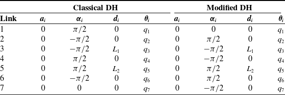

 x

 xi
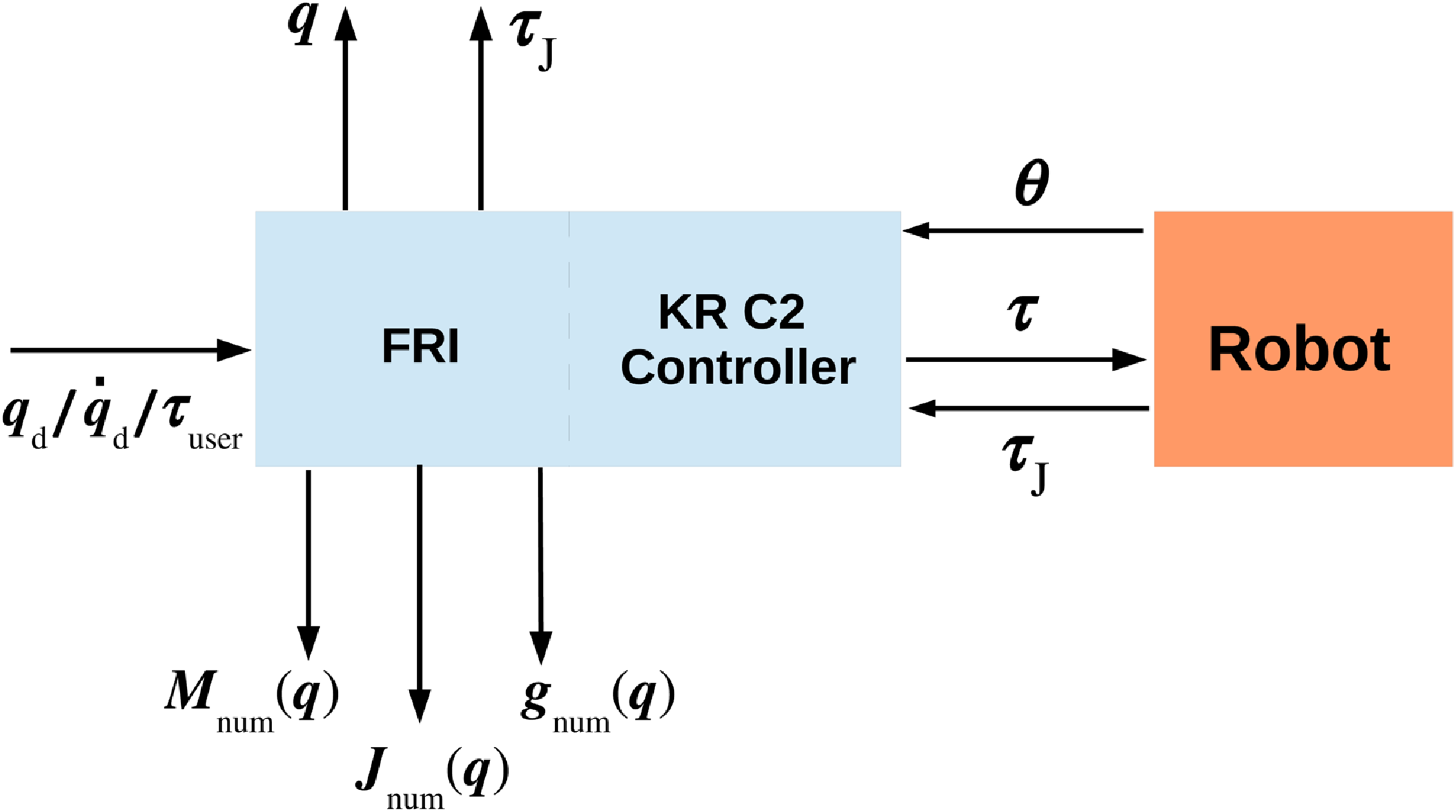

 m=1000
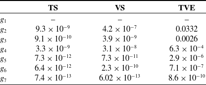
 g(q)
 g1
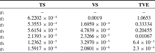
 g(q)
 g1
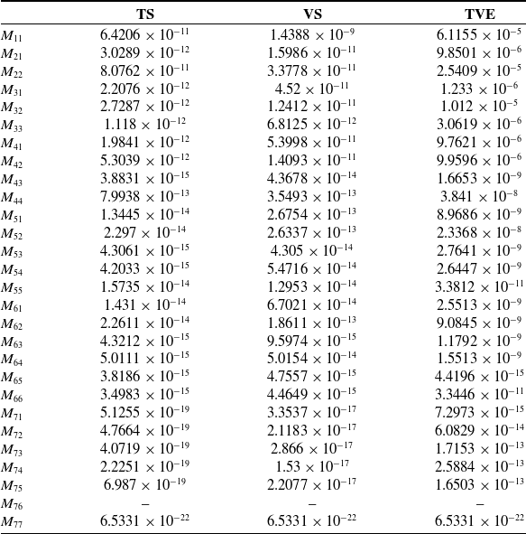
 M(q)
 M76
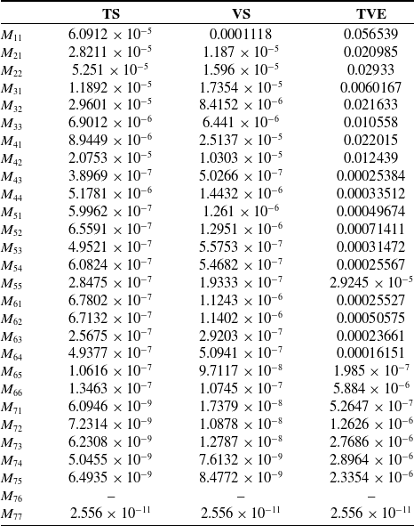
 M(q)
 M76

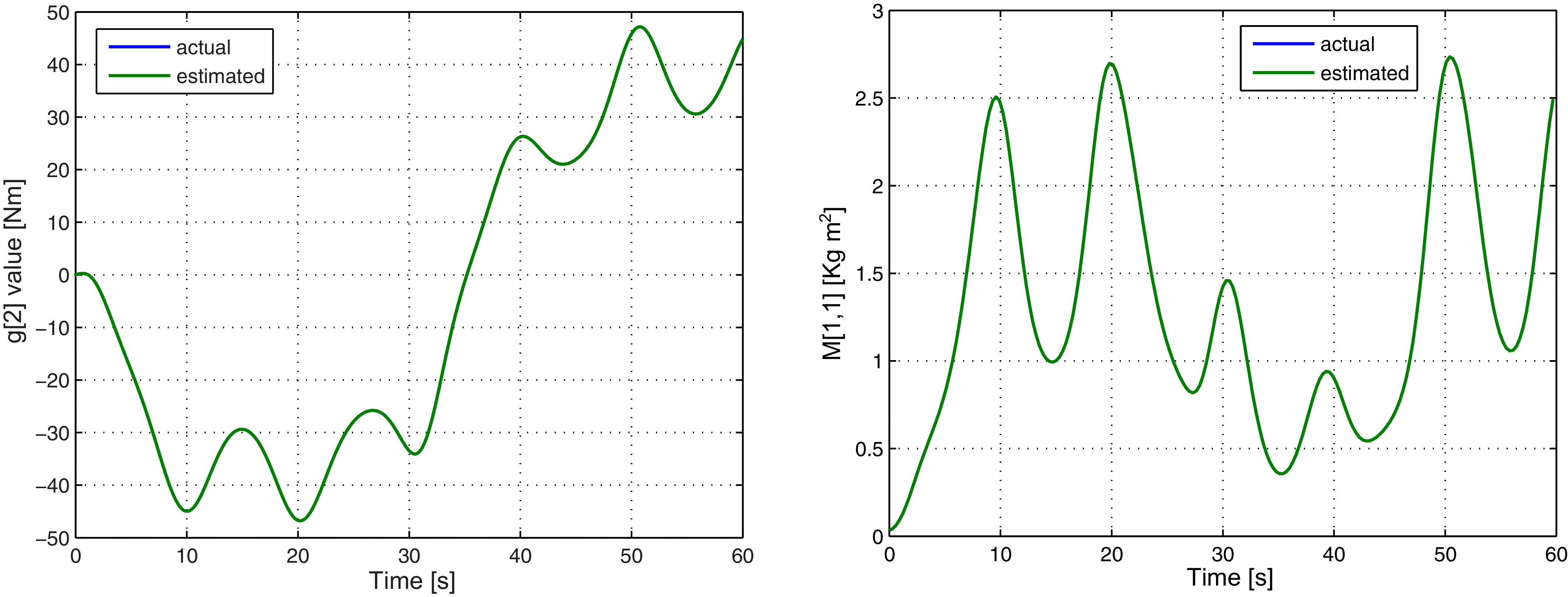
 g2(q)
 M11(q)

 t∈[0,30]
 t=22

 τJ
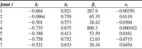
 τfl,i

 τfl
 τJ
 τ^J

 τJ
 τ^J
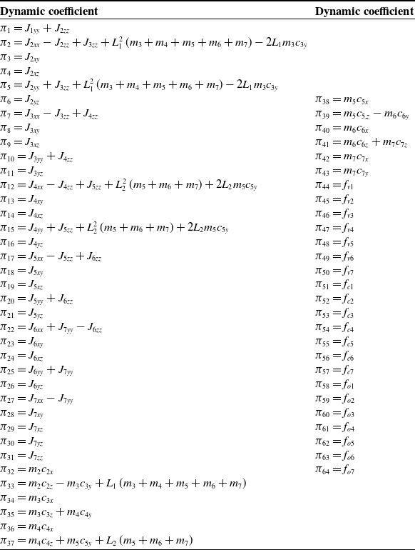
 64
 πc(pc)
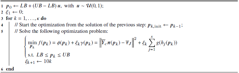
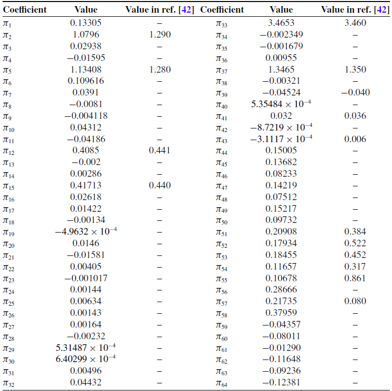
 64
 πc
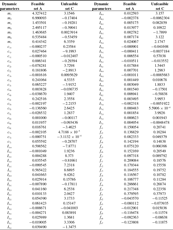
 91
 pc
 i=1,…,7
 mi
 cij
 j=x,y,z
 Iijk
 j=x,y,z
 k=x,y,z
 ⋅
 2
 fv,i
 ⋅
 fc,i
 fo,i

 p^c=p^A
 τJ
 τ^J

 fi


 ei=qdi−qi
 i=1,…,7
 ‖e‖

 τFB,i
 i=1,…,7
 ‖τFB‖

 ei=qdi−qi
 i=1,…,7
 ‖e‖

 τFB,i
 i=1,…,7
 ‖τFB‖

 τcommI
 τJ
 g^(qd)

 δi
 i=1,…,7
 τcommIII
 +
 −
 q˙i

 ei=qdi−qi
 i=1,…,7
 ‖e‖

 τFB,i
 i=1,…,7
 ‖τFB‖


 t=1.5
 8
 17
 3
 6

 r^(t)
 t=29

 q(t)
 t=29


 Open access

