1 Introduction
In short, dynamical system theory is the study of motion and we want to understand the behaviour of most orbits. Typically, the structure of the orbits is very complicated, for example, in some cases, there are orbits that almost fill the whole space, making it indecomposable from the dynamical point of view. That is what is called transitivity: a dynamical system is said to be transitive if it has a dense forward orbit. Even more interesting are the systems that present a dynamical feature that is stable or robust (meaning that it persists under perturbation). We say that a dynamical system is robustly transitive if there is a neighbourhood of the system (in some particular topology) such that every system in this neighbourhood is transitive.
The first example of a
 $C^1$
robustly transitive diffeomorphism was given by Anosov in [Reference Anosov1], where he proved that uniformly hyperbolic diffeomorphisms (today called Anosov diffeomorphisms) are stable under
 $C^1$
perturbations. As a corollary, every transitive Anosov diffeomorphism is in fact
 $C^1$
robustly transitive. Years later, Shub [Reference Shub17] constructed the first non-Anosov
 $C^1$
robustly transitive diffeomorphism on the torus
 ${\mathbb T}^4$
and later, R. Mañé improved this result and introduced an example on
 ${\mathbb T}^3$
[Reference Mañé14]. Both Shub’s and Mañé’s examples are isotopic to linear Anosov diffeomorphisms and for that reason, they are called derived from Anosov examples (from now on, DA diffeomorphisms). Another way to construct
 $C^1$
robustly transitive diffeomorphisms was introduced by Bonatti and Díaz in [Reference Bonatti and Díaz3]. Their technique is based on the existence of some particular hyperbolic subsets called blenders. With this geometric approach, the authors were able to build examples
 $C^1$
-close to time-t maps of Anosov flows (hence, isotopic to the identity) as well as examples
 $C^1$
-close to the product of Anosov times the identity (therefore, with trivial action on the centre). All these non-hyperbolic examples are partially hyperbolic (although there are also
 $C^1$
robustly transitive examples that are not partially hyperbolic [Reference Bonatti and Viana4]).
In [Reference Pujals and Sambarino16], Pujals and Sambarino introduced the SH property (some hyperbolicity) for partially hyperbolic diffeomorphisms. This property, which is
 $C^1$
robust, in addition to minimality of the strong stable foliation, implies
 $C^1$
robust minimality of the strong stable foliation; therefore,
 $C^1$
robust transitivity. As an application of this approach, they re-obtained the examples of Shub and Mañé.
Our contribution in this article is the introduction of a more general concept of SH property that we called the SH-saddle property. This new definition is a natural generalization of the previous SH definition and, as a consequence, it can be applied to a larger number of cases. In particular, it has the advantage of being applicable in the symplectic context (something that the previous definition could not be).
Let us be more precise. We say that a diffeomorphism
 $f:M \to M$
is partially hyperbolic if there exists a non-trivial
 $Df$
-invariant splitting
 $TM=E_f^{ss} \oplus E_f^c \oplus E_f^{uu}$
of the tangent bundle and numbers
 $\unicode{x3bb} _s,\unicode{x3bb} _c^-, \unicode{x3bb} _c^+, \unicode{x3bb} _u$
with
 $\unicode{x3bb} _s <1< \unicode{x3bb} _u$
and
 $\unicode{x3bb} _s < \unicode{x3bb} _c^- < \unicode{x3bb} _c^+\,{<}\, \unicode{x3bb} _u$
such that

We will denote by
 ${\mathcal {PH}}(M)$
the set of all partially hyperbolic diffeomorphisms of M. It is well known that the strong bundles
 $E_f^{uu}$
and
 $E_f^{ss}$
integrate into unique invariant foliations
 ${\mathcal W}^{uu}_f$
and
 ${\mathcal W}^{ss}_f$
, respectively, called the strong unstable and strong stable foliations [Reference Hirsch, Pugh and Shub11]. For
 $* = uu,ss$
, and for any
 $x \in M$
, we denote by
 ${\mathcal W}_f^*(x)$
the leaf of
 ${\mathcal W}_f^*$
through x. In the following, for any
 $*\in \{ss,uu\}$
, we denote by
 $d_{\mathcal {W}_f^*}$
the leafwise distance, and for any
 $x \in M$
and for any
 $\epsilon>0$
, we denote by
 ${\mathcal W}_f^*(x,\varepsilon ):=\{y \in {\mathcal W}_f^*(x): d_{{\mathcal W}_f^*}(x,y)< \varepsilon \}$
the
 $\varepsilon $
-ball in
 ${\mathcal W}_f^*$
of centre x and radius
 $\varepsilon $
.
Now, given a
 $\mathbb {R}$
-vector space V with an inner product, we say that a cone in V is a subset
 ${\mathcal C}$
such that there is a non-degenerate quadratic form
 $B:V \to \mathbb {R}$
such that
 ${{\mathcal C}=\{v\in V: B(v)\leq 0\}}$
. Analogously, we can express the cone
 ${\mathcal C}$
according to a decomposition
 $V=E\oplus F$
:
 $$ \begin{align*} {\mathcal C}=\{v=(v_E,v_F): \lVert v_E\rVert\leq \theta \lVert v_{F}\rVert\} \end{align*} $$
for some
 $\theta>0$
. In this case, we observe that
 $B(v)=-\theta ^2\lVert v_{F}\rVert ^2+\lVert v_{E}\rVert ^2$
. We are going to say that the number
 $\theta $
in the equation above is the size of the cone. In some cases, we will note by
 ${\mathcal C}_{\theta }$
instead of
 ${\mathcal C}$
to emphasise the size of
 ${\mathcal C}$
. The dimension of a cone is the maximal dimension of any subspace contained in the cone.
Finally, given
 $f\in {\mathcal {PH}}(M)$
, we are going to say that a d-centre cone in
 $x\in M$
is simply a cone
 ${\mathcal C}(x)$
in
 $E^{c}_f(x)$
of dimension
 $d\leq \dim E^c_f$
.
We now introduce the main definition of the article.
Definition 1.1. (SH-saddle property for unstable foliations)
Given
 $f\in {\mathcal {PH}}(M)$
, we say that the strong unstable foliation
 ${\mathcal W}^{uu}_f$
has the
 $SH$
-saddle property of index
 $d\leq \dim E^c_f$
if there are constants
 $L>0$
,
 $\theta>0$
,
 $\unicode{x3bb} _0>1$
and
 $C>0$
such that the following hold. For every point
 $x\in M$
, there is a point
 $y\in {\mathcal W}^{uu}_f(x,L)$
such that the following hold.
-
(1) There is a d-centre cone field of size
 $\theta $
along the forward orbit of y which is
$Df$
-invariant, that is, there exist
${\mathcal C}^u_{\theta }(f^l(y))\kern1.3pt{\subset}\kern1.3pt E^c_f(f^l(y))$
such that
$Df({\mathcal C}^u_{\theta } (f^l(y)))\kern1.3pt{\subset} {\mathcal C}^u_{\theta }(f^{l+1}(y))$
for every
$l\geq 0$
.
-
(2)
$\lVert Df^n_{f^l(y)}(v)\rVert \geq C\unicode{x3bb} _0^n\lVert v\rVert $
for every
$v\in {\mathcal C}^u_{\theta }(f^{l}(y))$
and every
$l,n\geq 0$
.





Notice that if the strong unstable foliation has SH-saddle property of index
 $d=\dim E^c_f$
, we get the original definition of SH property introduced in [Reference Pujals and Sambarino16]. The only difference is that we express the uniform expanding behaviour in the centre bundle in terms of a cone criterion. This allows us to treat the case where there is expansion in a subbundle of the centre subspace instead of the whole centre bundle. Moreover, since properties that are presented in terms of cones are, in general, robust in the
 $C^1$
topology, we are able to prove that this new SH-saddle property is
 $C^1$
open among partially hyperbolic diffeomorphisms (Theorem 2.8).
We can make an analogous definition of SH-saddle property for the strong stable foliation. In this case, we ask for the invariance of the cones for the past.
Definition 1.2. (SH-saddle property for stable foliations)
Given
 $f\in {\mathcal {PH}}(M)$
, we say that the strong stable foliation
 ${\mathcal W}^{ss}_f$
has the
 $SH$
-saddle property of index
 $d\leq \dim E^c_f$
if there are constants
 $L>0$
,
 $\theta>0$
,
 $\unicode{x3bb} _{0}>1$
and
 $C>0$
such that the following hold. For every point
 $x\in M$
, there is a point
 $y\in {\mathcal W}^{ss}_f(x,L)$
such that the following hold.
-
(1) There is a d-centre cone field of size
$\theta $
along the backward orbit of y which is
$Df^{-1}$
-invariant, that is, there exist
${\mathcal C}^s_{\theta }(f^l(y))$
such that
$Df^{-1}({\mathcal C}^s_{\theta }(f^l(y)))\subset {\mathcal C}^s_{\theta }(f^{l-1}(y))$
for every
$l \leq 0$
. -
(2)
$\lVert Df^n_{f^l(y)}(v)\rVert \geq C\unicode{x3bb} _0^{-n}\lVert v\rVert $
for every
$v\in {\mathcal C}^s_{\theta }(f^l(y)))$
and every
$l,n\leq 0$
.


With this new approach, we first give a sufficient condition for a DA diffeomorphism to be
 $C^1$
robustly transitive (Theorem 3.8). As an application of this result, we are able to build new
 $C^1$
robustly transitive DA diffeomorphisms, in particular, with any centre dimension and with as many different behaviours on centre leaves as desired. Moreover, these examples can be made in a way such that they have mixed behaviour on centre leaves. In particular, they present a dominant splitting that is not coherent with the hyperbolic splitting of their linear Anosov part, a difference with its predecessor DA examples ([Reference Bonatti and Díaz3, Reference Bonatti and Viana4, Reference Mañé14, Reference Shub17]).
Theorem A. Let
 $n\geq 4$
and let
 $A\in \mathrm {SL}(n,{\mathbb Z})$
be a hyperbolic symmetric matrix with a splitting of the form
 ${\mathbb R}^n=E^{ss}_A\oplus E^{ws}_A\oplus E^{wu}_A \oplus E^{uu}_A$
. Denote by
 $E^c_A=E^{ws}_A\oplus E^{wu}_A$
and let
 $k=\dim E^c_A\geq 2$
. Then, there exist a
 $C^1$
robustly transitive partially hyperbolic diffeomorphism
 $f:{\mathbb T}^n\to {\mathbb T}^n$
, isotopic to A with a splitting of the form
 $T{\mathbb T}^n=E^{ss}_f\oplus E^c_f\oplus E^{uu}_f$
such that
 $\dim E^*_f=\dim E^*_A$
for
 $*=ss,c,uu$
, and with
 $k+1$
fixed points
 $p_0,p_1,\ldots ,p_k$
such that
 $\text {index}(p_j)=j+\dim E^{ss}_A$
for every
 $j=0,\ldots ,k$
.
Moreover, the centre bundle
 $E^c_f$
does not admit a dominant splitting. In particular, the splitting of f is not coherent with the hyperbolic splitting of A.
We remark that in the theorem above,
 $E^c_A$
is strictly hyperbolic, but the proof for the case where
 $E^c_A$
is entirely contracting or expanding works as well. In these last cases, the result is basically contained in [Reference Pujals and Sambarino16] with the difference of dealing with the minimality of the strong unstable foliation instead of transitivity.
Let us mention that in his PhD thesis, Potrie [Reference Potrie15, p. 152] constructed a
 $C^1$
robustly transitive example on
 ${\mathbb T}^3$
, but in this case, the example’s dominant splitting is not coherent with its Anosov part, although the definition of partial hyperbolicity here is a bit different. Recently, Carrasco and Obata showed in [Reference Carrasco and Obata6] that the example introduced in [Reference Berger and Carrasco2] is
 $C^1$
robustly transitive. This example, although it is a skew product on
 ${\mathbb T}^4$
, has the particularity of having mixed behaviour on the centre (which is two-dimensional) and therefore makes it a new example. The authors mention in the paper that their example cannot have the SH property (the original version). However, it follows directly from the calculations in their article that the example has the SH-saddle property. Therefore, at the moment, every known example of
 $C^1$
robustly transitive partially hyperbolic diffeomorphism verifies the SH-saddle property of some index.
In addition to the examples in Theorem A, we also present two additional examples of
 $C^1$
robustly transitive partially hyperbolic diffeomorphisms. These examples are, in a sense, similar to those in Theorem A, but with a different flavour. The first one has the particularity of being symplectic and it has the SH-saddle property. Recall that the original SH property is incompatible with being symplectic, so this example shows that the SH-saddle property is useful in the symplectic context. The second example is different to the last ones since the set of points of the manifolds where hyperbolicity fails is not localized in small neighbourhoods of fixed points.
Finally, let us mention that the robust minimality of the strong foliations, which is the main purpose of the original SH definition in [Reference Pujals and Sambarino16], is out of reach, since the same strategy Pujals and Sambarino made is not adaptable to the saddle case, and some new approach is needed. In fact, just the minimality of the strong foliations for a DA diffeomorphism, like those in Theorem A, is not easy to get, since even for true Anosov diffeomorphisms, this is a very difficult problem. Recently, it was announced by Avila, Crovisier, Eskin, Potrie, Wilkinson and Zhang that
 $\mathcal {W}^{uu}$
is minimal for every
 $C^{1+\alpha }$
Anosov diffeomorphism of
 ${\mathbb T}^3$
.
We end this introduction by presenting a few questions to which at the moment, we do not know the answers.
Question 1.3. Is it possible to obtain a criterion for the
 $C^1$
robust minimality of the strong foliations in the SH-saddle case, as that obtained by Pujals and Sambarino in [Reference Pujals and Sambarino16]?
Question 1.4. Does every
 $C^1$
robustly transitive partially hyperbolic diffeomorphism verify the SH-saddle property of some index?
Question 1.5. Does transitivity in addition to the SH-saddle property imply
 $C^1$
robust transitivity?
1.1 Organization of the paper
In §2, we prove that the SH-saddle property is a
 $C^1$
open condition among partially hyperbolic diffeomorphisms. In §3, we present a criterion for DA diffeomorphisms that guarantees
 $C^1$
robust transitivity. Finally, in §4, we apply the previous results to build new DA examples and prove Theorem A.
2 SH-saddle property is
$C^1$
open

The Definitions 1.1 and 1.2 of the SH-saddle property are given for the strong unstable and strong stable foliations, respectively. In many parts of the article, we will need the presence of the two simultaneously, thus for simplicity, we give the following definition of the SH-saddle property for diffeomorphisms by grouping together these two.
Definition 2.1. (SH-saddle property for diffeomorphisms)
We say that
 $f\in {\mathcal {PH}}(M)$
has
 $(d_1,d_2)$
SH-saddle property if the following conditions hold:
-
(1)
${\mathcal W}^{ss}_f$
has the
$SH$
-saddle property of index
$d_1$
; -
(2)
${\mathcal W}^{uu}_f$
has the
$SH$
-saddle property of index
$d_2$
.


Remark 2.2. Notice that, not necessarily, we have
 $d_1+d_2=\dim E^c_f$
, in fact, in many cases, we are going to have
 $d_1+d_2<\dim E^c_f$
. For simplicity, in some parts of the article, we are going to omit the indices
 $(d_1,d_2)$
and we are just going to say that a partially hyperbolic diffeomorphism has the SH-saddle property.
Remark 2.3. The SH-saddle property does not depend on the choice of the Riemannian metric.
As a consequence of the previous remark, we get the following fact.
Proposition 2.4. A partially hyperbolic diffeomorphism f has the SH-saddle property if and only if
 $f^N$
has the SH-saddle property for some
 $N\in {\mathbb N}$
.
Let us introduce some notation that will be useful in the article and will help us to get a better understanding of what the SH-saddle property means. Let
 $f\in {\mathcal {PH}}(M)$
be such that its unstable foliation has the SH-saddle property of index
 $d\leq \dim E^c_f$
and let
 $L>0$
,
 $\theta>0$
,
 $\unicode{x3bb} _0>1$
and
 $C>0$
be the constants given by Definition 1.1. We can define the following subset:

Then, the unstable foliation has the SH-saddle property of index d if and only if

In the same way, let
 $f \in {\mathcal {PH}}(M)$
be such that its stable foliation has the SH-saddle property of index d and let
 $L>0$
,
 $\theta>0$
,
 $\unicode{x3bb} _0>1$
and
 $C>0$
be the constants given by Definition 1.2, then we can define the following subset:

and the stable foliation has the SH-saddle property of index d if and only if

Remark 2.5. The sets
 $H^{*}_{\unicode{x3bb} _0,d}(f)$
are closed subsets of M for
 $*=+,-$
.
In the reminder of this section, we are going to prove that the SH-saddle property is
 $C^1$
open among
 ${\mathcal {PH}}(M)$
. According to Definition 2.1, we only have to prove that having an unstable manifold with the SH-saddle property, Definition 1.1, and having a stable manifold with the SH-saddle property, Definition 1.2, are
 $C^1$
open properties. We are going to focus on the unstable case, since the stable case is completely symmetric. We begin with a few simple lemmas that only use the properties of the
 $C^1$
topology.
Lemma 2.6. Suppose that the unstable foliation of
 $f\in {\mathcal {PH}}(M)$
has SH-saddle property of index d. Then, there is
 $\delta _0>0$
such that if
 $d(y,H^+_{\unicode{x3bb} _0,d}(f))<\delta _0$
, then y and
 $f(y)$
have d-centre cones
 ${\mathcal C}^u(y)$
and
 ${\mathcal C}^u(f(y))$
such that
 $Df({\mathcal C}^u(y))\subseteq {\mathcal C}^u(f(y))$
.
Proof. We know that for every
 $x\in H^+_{\unicode{x3bb} _0,d}(f)$
, there is a cone
 ${\mathcal C}^u(x)$
which is
 $Df$
-invariant. Now, for the first part of the lemma, just notice that since the family of centre cones comes from a non-degenerate quadratic form, we can extend this quadratic form to neighbours by continuity. For the invariance, just observe that
 $Df$
is uniformly continuous.
Since the family of cones varies continuously, the same family of cones in the lemma above is still invariant for every g sufficiently
 $C^1$
close to f. Then, we obtain the following lemma.
Lemma 2.7. Suppose that the unstable foliation of
 $f\in {\mathcal {PH}}(M)$
has the SH-saddle property of index d, and let
 $\delta _0>0$
be as in Lemma 2.6. Then, there is a
 $C^1$
-neighbourhood
 ${\mathcal U}_0(f)$
of f such that if
 $g\in {\mathcal U}_0(f)$
and
 $d(y,H^+_{\unicode{x3bb} _0,d}(f))<\delta _0$
, then
 $Dg({\mathcal C}^u(y))\subseteq {\mathcal C}^u(g(y))$
.
Now, we are ready to prove the main theorem of this section.
Theorem 2.8. Suppose that the unstable foliation of
 $f\in {\mathcal {PH}}(M)$
has the SH-saddle property of index d. Then, there are constants
 $\unicode{x3bb}>1$
,
 $L>0$
and a
 $C^1$
-neighbourhood
 $\mathcal {V}$
of f such that, if
 $g\in \mathcal {V}$
, then
 $H^+_{\unicode{x3bb} ,d}(g)\cap {\mathcal W}^{uu}_g(x,L)\neq \emptyset $
for every
 $x\in M$
(that is, the unstable foliation
 ${\mathcal W}^{uu}_g$
has the SH-saddle property of index d with constants
 $\unicode{x3bb}>1$
and
 $L>0$
).
Proof. Take
 $f\in {\mathcal {PH}}(M)$
such that its strong unstable foliation has the SH-saddle property of index d. That means there are constants
 $\unicode{x3bb} _0>1$
,
 $L_0>0$
and
 $C>0$
such that Definition 1.1 holds. Then, we have

Let
 $\delta _0>0$
and
 ${\mathcal U}_0(f)$
be as in Lemmas 2.6 and 2.7. Take
 $c>0$
such that
 ${\unicode{x3bb} _{0}}/({1+c}) = \unicode{x3bb} _{1}>1$
. Take
 ${\varepsilon }>0$
,
 $\delta _1\in (0,\delta _0)$
and
 $\mathcal {U}_{1}(f)\subseteq \mathcal {U}_{0}(f)$
such that if
 $g\in \mathcal {U}_{1}(f)$
,
 $d(x,y)<\delta _1$
and
 $v\in T_xM$
has
 $\lVert v\rVert =1$
, then
 $$ \begin{align*} \lVert Df_x(v)-Dg_y(w)\rVert<{\varepsilon}, \end{align*} $$
where
 $w=P_{x,y}(v) \in T_yM$
is the parallel transport of v from x to y. We can take
 ${\varepsilon }>0$
small enough such that if
 $d(x,y)<\delta _1$
and
 $g\in \mathcal {U}_{1}(f)$
, then
 $$ \begin{align} \frac{1}{1+c}\leq \frac{\lVert Df_x\rVert}{\lVert Dg_y\rVert} \leq 1+c \quad\text{and}\quad \frac{1}{1+c}\leq \frac{m\{Df_x\}}{m\{Dg_y\}} \leq 1+c. \end{align} $$
Finally, let
 $K^+=\sup \{\lVert Df|_{E^c(x)}\rVert : x\in M\}$
and
 $K^-=\inf \{ m\{Df|_{E^c(x)}\}: x\in M\}$
. We can assume that
 $K^+$
and
 $K^-$
are
 $C^1$
-uniform on a neighbourhood
 ${\mathcal U}_2(f)\subseteq {\mathcal U}_1(f)$
.
Let
 $m_1\in {\mathbb Z}^+$
be large enough such that

and moreover, for any
 $g\in {\mathcal U}_2(f)$
and any
 $x\in M$
, we have
 $$ \begin{align} {\mathcal W}^{uu}_g(g^{m_1}(x),L_0) \subset g^{m_1}({\mathcal W}^{uu}_g(x,\delta_1/4)). \end{align} $$
Now, take
 $m_2\in {\mathbb Z}^+$
sufficiently large and take
 $\unicode{x3bb} _2$
such that

Let
 ${\mathcal U}_3(f)$
and
 $\delta _2\in (0,\delta _1/2)$
be such that if
 $d(x,y)<\delta _2$
and
 $g\in {\mathcal U}_3(f)$
, then
 $d(f^j(x),g^j(y))<\delta _1$
for
 $0\leq j \leq m_2$
.
Finally, take
 ${\mathcal U}_4(f) \subset {\mathcal U}_3(f)$
such that for every
 $g \in {\mathcal U}_4(f)$
, we have

We claim that every
 $g\in \mathcal {V}={\mathcal U}_4(f)$
has unstable manifold with the SH-saddle property of index d. In fact, we are going to see that
 $g^{k_0}$
has this property for
 $k_0=m_1+m_2$
, with constants
 $L=2L_0$
and
 $\unicode{x3bb} _2>1$
(where
 $\unicode{x3bb} _2$
comes from equation (2.4)). Then, we conclude by Proposition 2.4.
To see this, take
 $g\in \mathcal {V}$
and
 $x\in M$
. We know there are points
 $x^u_0 \in H^+_{\unicode{x3bb} _0,d}(f)$
and
 ${z^u_0 \in {\mathcal W}^{uu}_g(x,L_0)}$
such that
 $d(x^u_0,z^u_0)<\delta _2$
. Notice that since
 $\delta _2<\delta _0$
, we know there is a centre cone
 ${\mathcal C}^u(z^u_0)$
.
Now, let
 $v \in {\mathcal C}^u(z^u_0)$
. Since
 $d(x^u_0,z^u_0)<\delta _2$
, we have that
 $d(f^j(x^u_0),g^j(z^u_0))<\delta _1$
for
 $0\leq j \leq m_2$
. Then, we have

where
 $w=P_{z^u_0,x^u_0}(v)$
is the parallel transport of v from
 $z^u_0$
to
 $x^u_0$
. Now,

Now, by (2.3), we can apply the same argument to
 ${\mathcal W}^{uu}_g(g^{k_0}(z^u_0),L_0)$
, and we can find points
 $x^u_1\in H^+_{\unicode{x3bb} _0,d}(f)$
and
 $z^u_1 \in {\mathcal W}^{uu}_g(g^{k_0}(z^u_0),L_0)$
such that
 $d(x^u_1,z^u_1)<\delta _2$
. Then, there is a centre cone
 ${\mathcal C}^u(z^u_1)$
and for every vector
 $v\in {\mathcal C}^u(z^u_1)$
, we have
 $\lVert Dg^{k_0}_{z^u_1}(v)\rVert \geq \unicode{x3bb} _2\lVert v\rVert $
. Call
 $y^u_1=g^{-k_0}(z^u_0)$
. Now, by equation (2.3), we have that
 $g^{-m_1}(z^u_1)\in {\mathcal W}^{uu}_g(g^{m_2}(y^u_1),\delta _1/4)$
and this implies that
 $$ \begin{align*}d(x^u_0,y^u_1)\leq d(x^u_0,y^u_0)+d(y^u_0,y^u_1)<\delta_2 +\frac{\delta_1}{4}\leq \frac{\delta_1}{2}+\frac{\delta_1}{4}<\delta_1 < \delta_0\end{align*} $$
and there is a d-centre cone
 ${\mathcal C}^u(y^u_1)$
. Moreover, we have that
 $$ \begin{align*} d(g^j(y^u_1),g^j(z^u_0))<\delta_1 \quad\text{for every } 0\leq j \leq m_2 \end{align*} $$
and by applying the same calculations as in equations (2.5) and (2.6), we have

Inductively, we can find sequences
 $\{z^u_n\}_{n\in {\mathbb N}}$
,
 $\{y^u_n\}_{n\in {\mathbb N}}$
and
 $\{x^u_n\}_{n\in {\mathbb N}}$
, which verify the following:
-
•
$z^u_{n}\in {\mathcal W}^{uu}_g(g^{k_0}(z^u_{n-1}),L_0)$
; -
•
$x^u_n\in H^+_{\unicode{x3bb} _0,d}(f)$
; -
•
$d(z^u_n,x^u_n)<\delta _2$
; -
•
$y^u_n=g^{-k_{0}n}(z^u_n)$
.


Notice that since
 $z^u_{n}\in {\mathcal W}^{uu}_g(g^{k_0}(z^u_{n-1}),L_0)$
, we have
 $d(g^{-k_0}(z^u_n),z^u_{n-1})<\delta _1/4$
by equation (2.3). Then, by equation (2.2), we have
 $$ \begin{align*} d(y^u_{n-1},y^u_n)&=d(g^{-k_0(n-1)}(z^u_{n-1}),g^{-k_0n}(z^u_n)) \\ &=d(g^{-k_0(n-1)}(z^u_{n-1}), g^{-k_0(n-1)}(g^{-k_0}(z^u_n)) \leq \frac{\delta_1}{4} \bigg( \frac{1}{2} \bigg)^{n-1} =\delta_1 \bigg( \frac{1}{2} \bigg)^{n+1}. \end{align*} $$
By the triangular inequality, the distance between
 $x^u_0$
and
 $y^u_n$
is
 $$ \begin{align*} d(x^u_0,y^u_n) \leq d(x^u_0,y^u_0)+\sum_{j=1}^{n} d(y^u_{j-1},y^u_j)\leq \delta_2+\sum_{j=1}^{n} \delta_1 \bigg(\frac{1}{2} \bigg)^{j+1} < \sum_{j=0}^{n} \bigg(\frac{1}{2} \bigg)^{j+1}\delta_1 <\delta_1 \end{align*} $$
since
 $\delta _2 <\delta _1/2$
. Then, there is a d-centre cone
 ${\mathcal C}^u(g^j(y^u_n))$
such that
 $Dg({\mathcal C}^u(g^j(y^u_n))) \subset {\mathcal C}^u(g^{j+1}(y^u_n))$
for every
 $j\in \{0,\ldots ,nk_0\}$
. Moreover,
 $y^u_n\in {\mathcal W}^{uu}_g(x,2L_0)$
.
By the same reasons as above, if
 $v\in {\mathcal C}^u(g^{ik_0}(y^u_n))$
, we have

Finally, if we take
 $y \in {\mathcal W}^{uu}_g(x,2L_0)$
as an accumulation point of
 $\{y^u_n\}_{n\in {\mathbb N}}$
, we obtain that there is a d-centre cone
 ${\mathcal C}^u(g^l(y))\subset E^c_g(g^l(y))$
such that
 $Dg({\mathcal C}^u(g^l(y)))\subset {\mathcal C}^u(g^{l+1}(y))$
for every
 $l\geq 0$
and
 $\lVert Dg^{jk_0}(v)\rVert \geq \unicode{x3bb} _2^j\lVert v\rVert $
, for every
 $v\in {\mathcal C}^u(g^{lk_0}(y))$
and
 $j,l>0$
.
Since the
 $C^1$
-openess of the SH-saddle property for stable manifolds is completely analogous, we get the following corollary.
Corollary 2.9. The SH-saddle property in equation (2.1) is
 $C^1$
open among
 ${\mathcal {PH}}(M)$
.
We end this section with a key corollary from Theorem 2.8 that we are going to use in the next sections. First, let us say that D is a centre disk of dimension
 $d\leq \dim E^c_f$
if it is a d-dimensional embedded disk contained in some centre plaque.
Corollary 2.10. Let
 $f\in {\mathcal {PH}}(M)$
be such that its unstable foliation has the SH-saddle property of index d and let
 $\unicode{x3bb}>1$
,
 $\delta _1>0$
and
 $\mathcal {V}$
as in Theorem 2.8. Take
 $g\in \mathcal {V}$
,
 $x^u \in H^+_{\unicode{x3bb} ,d}(g)$
and
 $D^u$
a centre disk of dimension d tangent to
 ${\mathcal C}^u(x^u)$
. Then, there is
 $N>0$
such that
 $g^n(D^u)$
contains a centre disk of dimension d, centred at
 $g^n(x^u)$
of diameter bigger than
 $2\delta _1$
for every
 $n\geq N$
.
Analogously with the stable foliation.
Proof. First, recall that
 $\mathcal {U}_1(f)$
and
 $\delta _1>0$
come from equation (2.1). Then, just notice that if
 $g\in \mathcal {V}\subseteq \mathcal {U}_1(f)$
and
 $d(x,x^u)<\delta _1$
, then their distance is expanded by
 $\unicode{x3bb}>1$
for the future in the
 $\mathcal {C}^u$
direction. In particular, their distance in the centre leaf is
 $d(g(x),g(x^u))\geq \unicode{x3bb} d(x,x^u)\geq \unicode{x3bb} \delta _1>\delta _1$
. Then, no matter how small is the centre disk
 $D^u$
, eventually by induction, we obtain a centre disk with diameter bigger than
 $2\delta _1$
.
3 Derived from Anosov revisited
In this section, we are going to present a sufficient condition for derived from Anosov diffeomorphisms to be
 $C^1$
robustly transitive. We begin by explaining what we mean by derived from Anosov diffeomorphisms.
Take
 $n\in {\mathbb N}$
with
 $n\geq 4$
and let
 $p:{\mathbb R}^n\to {\mathbb R}^n/{\mathbb Z}^n={\mathbb T}^n$
be the canonical projection. Take
 $A\in \text {SL}(n,{\mathbb Z})$
a hyperbolic matrix with a dominant splitting of the form
 $$ \begin{align} {\mathbb R}^n=E^{ss}_A\oplus E^{ws}_A\oplus E^{wu}_A\oplus E^{uu}_A \end{align} $$
and denote by
 $f_A$
the linear Anosov diffeomorphism induced in the torus
 ${\mathbb T}^n$
, that is,
 $f_A \circ p =p\circ A$
. By a slight abuse of notation, we are going to note
 $f_A=A$
. In addition to this decomposition, we can group together the two middle bundles and call
 $E^c_A=E^{ws}_A\oplus E^{wu}_A$
the centre bundle. This way, we get a dominant splitting of the form
 $$ \begin{align*}{\mathbb R}^n=E^{ss}_A\oplus E^{c}_A\oplus E^{uu}_A.\end{align*} $$
With this splitting, we can think of A as a partially hyperbolic diffeomorphism too. We say that
 $f:{\mathbb T}^n\to {\mathbb T}^n$
is a derived from Anosov diffeomorphism if it is isotopic to A. Now, we let
 ${\mathcal {PH}}_A({\mathbb T}^n)$
be the set
 $$ \begin{align*} {\mathcal{PH}}_{A}(\mathbb{T}^n)= \{ f \in {\mathcal{PH}}(\mathbb{T}^n): f \simeq A, \ \dim E^{*}_{f}=\dim E^{*}_{A} \ \text{for} \ *=ss,c,uu \}, \end{align*} $$
where
 $f\simeq A$
means the maps are isotopic. Then,
 ${\mathcal {PH}}_{A}(\mathbb {T}^n)$
is the set of partially hyperbolic derived from Anosov diffeomorphisms, such that the dimensions of the subbundles coincide with the dimensions of the linear subbundles. By the results of [Reference Fisher, Potrie and Sambarino8], we know that every
 $f\in {\mathcal {PH}}_{A}(\mathbb {T}^n)$
is dynamically coherent, that is, the bundles
 $E^{ss}_f\oplus E^c_f$
,
 $E^c_f\oplus E^{uu}_f$
and
 $E^c_f$
integrate to invariant foliations denoted by
 ${\mathcal W}^{cs}_f$
,
 ${\mathcal W}^{cu}_f$
and
 ${\mathcal W}^{c}_f$
, respectively.
3.1 Derived from Anosov with SH-saddle property
In this subsection, we are going to show that for every linear Anosov
 $A:{\mathbb T}^n\to {\mathbb T}^n$
as above, there is a derived from Anosov diffeomorphism with the SH-saddle property with a given index (actually the same index as its linear part).
Lemma 3.1. Let
 $A\in \mathrm {SL}(n,{\mathbb Z})$
be a hyperbolic matrix with a dominant splitting as in equation (3.1). Take
 ${\varepsilon }>0$
and call
 $U=B(0,{\varepsilon }) \subset {\mathbb T}^n={\mathbb R}^n/{\mathbb Z}^n$
. Take
 $f_t:{\mathbb T}^n\to {\mathbb T}^n$
an isotopy such that:
-
(1)
$f_0=A$
and
$f_1=f$
; -
(2)
$f_t|_{U^c}=A|_{U^c}$
for every
$t\in [0,1]$
; -
(3)
$\dim E^{*}_{f_t}=\dim E^{*}_{A}$
for every
$*=ss,c,uu$
and every
$t\in [0,1]$
.


Then, if
 ${\varepsilon }$
is sufficiently small,
 $f\in {\mathcal {PH}}_A({\mathbb T}^n)$
has the
 $(d_1,d_2)$
SH-saddle property, where
 $d_1=\dim E^{ws}_A$
and
 $d_2=\dim E^{wu}_A$
.
Proof. Take f as in the hypothesis. We can assume that
 ${\varepsilon }$
is small enough to send
 $f_t$
to the quotient
 ${\mathbb T}^n={\mathbb R}^n/{\mathbb Z}^n$
. It is clear that a diffeomorphism f built this way belongs to
 ${\mathcal {PH}}_A({\mathbb T}^n)$
. By taking an iterate, we can suppose that
 $\lVert Df_{x}|_{E^{uu}_f(x)}\rVert>4$
for every
 ${x\in {\mathbb T}^n}$
. Now take
 $0<\epsilon <1/4$
. Then, for every
 $x\in {\mathbb T}^n$
, there is a point
 $z^{x}_0 \in \mathcal {W}^{uu}_{f}(x,1)$
such that
 $\mathcal {W}^{uu}_{f}(z^{x}_0,1/4)\cap U =\emptyset $
. Call
 ${\mathcal D}_{0}=\overline {\mathcal {W}^{uu}_{f}(z^{x}_0,1/4)}$
. In the same way, since
 $f({\mathcal D}_{0})\supseteq \mathcal {W}^{uu}_{f}(f(z^x_0),1)$
, we can find a disk
 ${\mathcal D}_{1}=\overline {\mathcal {W}^{uu}_f(z^{x}_1,1/4)} \subset f({\mathcal D}_0)$
such that
 ${\mathcal D}_1\cap U=\emptyset $
. Inductively, we get a sequence of unstable disks
 $\{{\mathcal D}_j\}_{j\geq 0}$
such that
 ${\mathcal D}_j\cap U=\emptyset $
for every
 $j\geq 0$
and
 $f^{-1}({\mathcal D}_j) \subset {\mathcal D}_{j-1}$
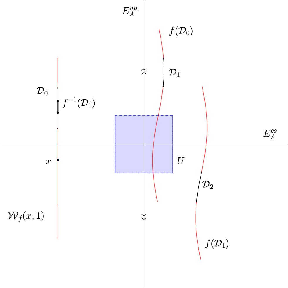
(see Figure 1 above). Finally, the point
 $x^u=\bigcap _{j\geq 0}f^{-j}({\mathcal D}_j)$
never meets U in the future. Since f is equal to A outside U, we get that the point
 $x^u$
is hyperbolic for the future, and so the unstable manifold
 ${\mathcal W}^{uu}_f$
has the SH-saddle property of index
 $d_2$
.
Finding a point whose forward orbit never meets U (colour online).

In the same way, we can find a point
 $x^s$
in every strong stable leaf of large 1, such that the past orbit of
 $x^s$
never meets U. Once again, since
 $f=A$
outside U, the same argument as above shows that
 ${\mathcal W}^{ss}_f$
has the SH-saddle property of index
 $d_1$
.
3.2 A criterion for openess
In this subsection, we present a result that we are going to apply for the proof of the main theorem. Roughly speaking, it says that given a continuous function between topological spaces of the same dimension, and such that the fibres (preimages of points) of the function are small enough, then the image of the function must contain an open set. The version we are going to use comes from [Reference Leguil and Zhang12], which is an improvement from a result of [Reference Bonk and Kleiner5, Proposition 3.2]. We begin with a few definitions.
Definition 3.2. Suppose
 $f:X\to Y$
is a continuous function between metric spaces. We say that
 $y\in Y$
is a stable value if there is
 $\epsilon>0$
such that if
 $d_{C^0}(f,g)<\epsilon $
, then
 ${y\in Im(g)}$
.
Remark 3.3. Let
 $Y=\mathbb {R}^n$
and suppose that
 $f:X \to \mathbb {R}^n$
has a stable value y, then
 $Im(f)$
contains an open set. To see this, take
 $\epsilon>0$
from the definition of stable value, and take a vector
 $v\in \mathbb {R}^d$
with
 $\lVert v\rVert <\epsilon $
. Then, the map
 $g:X\to \mathbb {R}^d$
defined by
 $g(x)=f(x)-v$
satisfies
 $d_{C^0}(f,g)= \lVert v\rVert <\epsilon $
. Since y is a stable value, there is a point
 $x\in X$
such that
 $g(x)=y$
and this is equivalent to
 $f(x)=y+v$
. Since v was arbitrary, we get
 $B_{\mathbb {R}^n}(y,\epsilon )\subset Im(f)$
.
Definition 3.4. Given a continuous function
 $f:X\to Y$
and
 $\rho>0$
, we say that f is
 $\rho $
-light if for every
 $y \in Y$
, the connected components of
 $f^{-1}(y)$
have diameter smaller than
 $\rho $
.
Proposition 3.5. [Reference Leguil and Zhang12, Theorem F]
Given
 $d\in \mathbb {N}$
and
 $r>0$
, there is
 $\rho =\rho (d,r)>0$
such that every
 $\rho $
-light map
 $f:[-r,r]^d\to \mathbb {R}^d$
has a stable value.
The version stated in [Reference Leguil and Zhang12] is for maps
 $f:[0,1]^d \to \mathbb {R}^d$
, but the proof can be adapted to maps
 $f:[-r,r]^d\to \mathbb {R}^d$
for a fixed
 $r>0$
. Now, combining this proposition and Remark 3.3, we have the following corollary.
Corollary 3.6. Fix
 $d\in \mathbb {N}$
and
 $r>0$
, and take the corresponding
 $\rho =\rho (d,r)>0$
from Proposition 3.5. Then, the image of every
 $\rho $
-light map
 $f:[-r,r]^d\to \mathbb {R}^d$
contains an open set.
3.3 Robust transitivity for DA diffeomorphisms
In this subsection, we are going to present a robust transitivity criterion for DA diffeomorphisms. This result will be used in the next section for the proof of Theorem A.
Let
 $A\in \text {SL}(n,{\mathbb Z})$
be a hyperbolic matrix with a dominant splitting as in equation (3.1). Take
 $f\in {\mathcal {PH}}_A({\mathbb T}^n)$
and let
 $\widetilde {f}$
be a lift to
 ${\mathbb R}^n$
. By [Reference Franks9], we know there exist a continuous and surjective map
 $H_f:{\mathbb R}^n \to {\mathbb R}^n$
such that
 $A \circ H_f=H_f\circ \widetilde {f}$
. The map
 $H_f$
is
 ${\mathbb Z}^n$
-invariant and, therefore, it induces a continuous and surjective map
 $h_f:{\mathbb T}^n\to {\mathbb T}^n$
such that
 $h_f \circ f=A \circ h_f$
. Moreover, the map
 $H_f$
varies continuously with the diffeomorphism f in the
 $C^0$
-topology and the distance
 $d_{C^0}(H_f ,\mathrm {Id}_{\widetilde {M}})=d_{C^0}(h_f,\mathrm {Id}_M)<\infty $
. In particular, we have that
 $d_{C^0}(H_f,\mathrm {Id}_{\widetilde {M}})\to 0$
when
 $f\to A$
in the
 $C^0$
topology.
Notice that we are making an abuse of notation since the map
 $H_f$
is determined by
 $\widetilde {f}$
instead of f. However, this is not a problem since given two lifts
 $\widetilde {f}_1$
and
 $\widetilde {f}_2$
, there is an integer vector
 $v\in {\mathbb Z}^n$
such that
 $\widetilde {f}_1-\widetilde {f}_2=v$
and this implies that
 $H_{f_2}=H_{f_1}+w$
, where
 $w=-(A-\mathrm {Id})^{-1}(v)$
:
 $$ \begin{align*} H_{f_2} \circ \widetilde{f_2}(\widetilde{x}) &= H_{f_1}(\widetilde{f_2}(\widetilde{x}))+w=H_{f_1}(\widetilde{f_1}(\widetilde{x})-v)+w \\ &= H_{f_1}\circ \widetilde{f_1}(\widetilde{x})-v+w= A \circ H_{f_1}(\widetilde{x})-v+w \\ &= A(H_{f_1}(\widetilde{x})+w)-Aw +w-v = A \circ H_{f_2}(\widetilde{x}) -(A-\mathrm{Id})^{-1}(w)-v \\ &= A \circ H_{f_2}(\widetilde{x}). \end{align*} $$
Observe that the matrix
 $A-\mathrm {Id}$
is invertible since A is hyperbolic.
Now, given
 $f\in {\mathcal {PH}}_A({\mathbb T}^n)$
and
 $\widetilde {x}\in {\mathbb R}^n$
, we are going to call the fibre of
 $\widetilde {x}\in {\mathbb R}^n$
to the set
 $H_f^{-1}(H_f(\widetilde {x}))$
. By the previous observation, given two lifts
 $\widetilde {f}_1$
and
 $\widetilde {f}_2$
, there is a vector
 $w\in {\mathbb R}^n$
such that
 $H_{f_2}=H_{f_1}+w$
and this implies that
 $$ \begin{align*} H_{f_2}^{-1}(H_{f_2}(\widetilde{x})) = H_{f_1}^{-1}(H_{f_1}(\widetilde{x})) \end{align*} $$
and the fibre does not depend on the choice of the lift. As a result, we can define the function size of the fibre
 $$ \begin{align*}\Lambda: {\mathcal{PH}}_A({\mathbb T}^n)\times {\mathbb R}^n \to {\mathbb R}_{\geq 0}\quad\text{by}\quad \Lambda(f,\widetilde{x})=\text{diam}(H_f^{-1}(H_f(\widetilde{x}))). \end{align*} $$
We also denote by
 $$ \begin{align*} \Lambda(f)=\sup\{\Lambda(f,\widetilde{x}):\widetilde{x}\in {\mathbb R}^n\} \end{align*} $$
the supremum of sizes within all fibres. Since
 $d_{C^0}(H_f,\mathrm {Id}_{{\mathbb R}^n})<\infty $
, this supremum is always finite and we get a well-defined function
 $\Lambda : {\mathcal {PH}}_A({\mathbb T}^n) \to {\mathbb R}_{\geq 0}$
. Notice that f is conjugated to A if and only if
 $\Lambda (f)=0$
, since
 $H_f$
is always surjective and
 $\Lambda (f)=0$
is equivalent to injectivity.
It is easy to see that the function
 $\Lambda $
does not depend continuously on f; however, we have an upper semicontinuity property as the following lemma shows.
Lemma 3.7. Let
 $f\in {\mathcal {PH}}_A(\mathbb {T}^n)$
. Then, for every
 ${\varepsilon }>0$
, there exist
 $\delta>0$
such that if
 $d_{C^0}(f,g)<\delta $
, then
 $\Lambda (g)< \Lambda (f)+{\varepsilon }$
.
Proof. Take
 $f\in {\mathcal {PH}}_A({\mathbb T}^n)$
and
 ${\varepsilon }>0$
. Suppose by contradiction that the lemma is false. Then, for every
 $k>0$
, there is
 $g_k\in {\mathcal {PH}}_A({\mathbb T}^n)$
with
 $d_{C^0}(g_k,f)\leq 1/k$
, and points
 $\widetilde {x_k}, \widetilde {y_k} \in {\mathbb R}^n$
such that
 $d(\widetilde {x_k},\widetilde {y_k})\geq \Lambda (f)+{\varepsilon }$
and
 $H_{g_k}(\widetilde {x_k})=H_{g_k}(\widetilde {y_k})$
. We can assume that
 $\widetilde {x_k}\to \widetilde {x}$
and
 $\widetilde {y_k}\to \widetilde {y}$
, and as a consequence,
 $d(\widetilde {x},\widetilde {y})\geq \Lambda (f)+{\varepsilon }$
. Since the map
 $g\mapsto H_g$
is continuous, for every
 $\delta>0$
, there is
 $k_0>0$
such that for every
 $k\geq k_0$
, we have
 $d_{C^0}(H_{g_k},H_f)<\delta $
. Then, by the triangular inequality, we have
 $$ \begin{align*} d(H_f(\widetilde{x}),H_f(\widetilde{y})) & \leq d(H_f(\widetilde{x}),H_f(\widetilde{x_k}))+d(H_f(\widetilde{x_k}),H_{g_k}(\widetilde{x_k})) +d(H_{g_k}(\widetilde{x_k}),H_{g_k}(\widetilde{y_k})) \\ &\quad + d(H_{g_k}(\widetilde{y_k}),H_f(\widetilde{y_k}))+d(H_f(\widetilde{y_k}),H_f(\widetilde{y})) \\ & \leq d(H_f(\widetilde{x}),H_f(\widetilde{x_k}))+2\delta + d(H_f(\widetilde{y}),H_f(\widetilde{y_k})) \to 2\delta \end{align*} $$
and this implies
 $H_f(\widetilde {x})=H_f(\widetilde {y})$
, since
 $\delta $
was arbitrary. As a result, the points
 $\widetilde {x}$
and
 $\widetilde {y}$
belong to the same fibre which implies
 $d(\widetilde {x},\widetilde {y})\leq \Lambda (f)$
. However, then we have
 $\Lambda (f)+\epsilon \leq d(\widetilde {x},\widetilde {y}) \leq \Lambda (f)$
, which is a contradiction.
Recall that a diffeomorphism
 $f:M \to M$
is said to be transitive if there is
 $x\in M$
such that
 $\overline {{\mathcal O}^+ (f,x)}=M$
. Equivalently, f is transitive if for every pair of open sets U and V, there is
 $N\in \mathbb {Z}^+$
such that
 $f^N(U)\cap V \neq \emptyset $
.
Now, we are ready to prove the main theorem of this section.
Theorem 3.8. (Robust transitivity criterion)
Let
 $A\in \mathrm {SL}(n,{\mathbb Z})$
be a hyperbolic matrix with a dominant splitting as in equation (3.1). Take
 $f \in {\mathcal {PH}}_A({\mathbb T}^n)$
with
 $(d_1,d_2)$
SH-saddle property where
 $d_1=\dim E^{ws}_A$
and
 $d_2=\dim E^{wu}_A$
. Then, there is
 $\rho =\rho (f)>0$
such that if
 $\Lambda (f)<\rho $
, then f is
 $C^1$
robustly transitive. In fact,
 $C^1$
robustly topologically mixing.
Proof. Take
 $f \in {\mathcal {PH}}_A({\mathbb T}^n)$
with
 $(d_1,d_2)$
SH-saddle property, where
 $d_1=\dim E^{ws}_A$
and
 $d_2=\dim E^{wu}_A$
. Let
 $\mathcal {V}$
,
 $\unicode{x3bb}>1$
and
 $\delta _1>0$
be as in Theorem 2.8.
Let us define the following constants:
 $$ \begin{align*} \rho_s &= \rho(\dim(E^{ss}_A\oplus E^{ws}_A),\delta_1); \\ \rho_u &= \rho(\dim(E^{wu}_A\oplus E^{uu}_A),\delta_1); \\ \rho &= \min \{\rho_s,\rho_u\}, \end{align*} $$
where
 $\rho (*,\delta _1)$
are given by Proposition 3.5 for
 $*=\dim (E^{ss}_A\oplus E^{ws}_A), \dim(E^{wu}_A\oplus E^{uu}_A)$
. We claim that the theorem holds for this
 $\rho>0$
and for proving this, we are going to find a
 $C^1$
-neighbourhood
 ${\mathcal U}(f)$
of f such that every
 $g\in {\mathcal U}(f)$
is transitive.
First, notice that since
 $\Lambda (f)<\rho (f)$
, by Lemma 3.7 applied to
 ${\varepsilon }= \rho (f) - \Lambda (f)>0$
, we know there is
 $\delta _0>0$
such that if
 $d_{C^0}(f,g)<\delta _0$
, then
 $\Lambda (g)<\Lambda (f)+{\varepsilon }=\rho (f)$
.
Now, take
 ${\mathcal U}(f)=\mathcal {V}\cap \{g\in {\mathcal {PH}}_A({\mathbb T}^n): d_{C^0}(f,g)<\delta _0\}$
. We claim that every
 ${g\in {\mathcal U}(f)}$
is transitive (in fact, topologically mixing). To get transitivity, we have to prove that for any two open sets
 $U_1, U_2 \subset {\mathbb T}^n$
, there is
 $k \in {\mathbb Z}^+$
such that
 $g^k(U_1)\cap U_2 \neq \emptyset $
.
Take two points
 $x_1\in U_1$
and
 $x_2\in U_2$
, and let
 $k_1 \in {\mathbb N}$
be such that
 $g^{-k_1}(U_1)\supset {\mathcal W}^{ss}_g(g^{-k_1}(x_1),L)$
and
 $g^{k_1}(U_2)\supset {\mathcal W}^{uu}_g(g^{k_1}(x_2),L)$
. Take
 $x^s \in H^-_{\unicode{x3bb} ,d_1}(g) \cap {\mathcal W}^{ss}_g (g^{-k_1}(x_1),L)$
and
 $x^u \in H^+_{\unicode{x3bb} ,d_2}(g) \cap {\mathcal W}^{uu}_g(g^{k_1}(x_2),L)$
given by
 $(d_1,d_2)$
SH-saddle property. Now, take
 $D^s \subset {\mathcal W}^c_g(x^s)$
a centre disk of dimension
 $d_1$
tangent to
 ${\mathcal C}^s(x^s)$
and
 $D^u \subset {\mathcal W}^c_g(x^u)$
a centre disk of dimension
 $d_2$
tangent to
 ${\mathcal C}^u(x^u)$
. We can take
 $D^s, D^u$
small enough such that
 $D^s \subset g^{-k_1}(U_1)$
and
 $D^u \subset g^{k_1}(U_2)$
. Recall that
 ${\mathcal C}^s$
and
 ${\mathcal C}^u$
are the cones invariant for the past and the future, respectively, given by the SH-saddle property. Moreover,
 ${\mathcal C}^s$
and
 ${\mathcal C}^u$
uniformly expand vectors for the past and the future, respectively.
Now, take
 $D_1=\bigcup _{x\in D^s} {\mathcal W}^{ss}_g(x,l)$
and
 $D_2=\bigcup _{x\in D^u}{\mathcal W}^{uu}_g(x,l)$
. We can choose
 $l>0$
small enough such that
 $D_1 \subset g^{-k_1}(U_1)$
and
 $D_2 \subset g^{k_1}(U_2)$
. Notice that
 $D_1$
is a disk of dimension equal to
 $\dim(E^{ss}_A\oplus E^{ws}_A)$
and
 $D_2$
is a disk of dimension equal to
 $\dim(E^{wu}_A\oplus E^{uu}_A)$
. Now, by Corollary 2.10, there is
 $k_2\in {\mathbb N}$
such that
 $g^{-k}(D^s)$
contains a disk of diameter bigger than
 $2\delta _1$
and
 $g^k(D^u)$
contains a disk of diameter bigger than
 $2\delta _1$
for every
 $k\geq k_2$
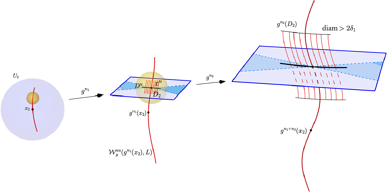
(see Figure 2).
Obtaining a disk of diameter bigger than
 $2\delta _1$
(colour online).

Now, let
 $\Pi ^{s}:{\mathbb R}^n\to E^{ss}_A\oplus E^{ws}_A$
and
 $\Pi ^{u}:{\mathbb R}^n\to E^{wu}_A\oplus E^{uu}_A$
be the orthogonal projections. Then, the idea is to use Corollary 3.6 applied to the functions
 $\Pi ^s \circ H_g$
and
 $\Pi ^u \circ H_g$
to conclude that for every
 $k\geq k_2$
, the images of the sets
 $g^{-k}(D_1)$
and
 $g^{k}(D_2)$
by
 $H_g$
contain topological disks of complementary dimensions and with the appropriate inclination. Then, the hyperbolicity of the matrix A will do the mixing, and we can translate this mixing of A to the diffeomorphism g.
Observe that
 $g \in {\mathcal U}(f)$
, which implies that
 $\Lambda (g)<\rho $
and, in particular, we have that
 $H_g$
is
 $\rho $
-light (see Definition 3.4). Moreover, we claim the following.
Claim 3.9. The function
 $\Pi ^{s}\circ H_g$
is
 $\rho $
-light when restricted to
 $\widetilde {g}^{-k}(\widetilde {D_1})$
and the function
 $\Pi ^u\circ H_g$
is
 $\rho $
-light when restricted to
 $\widetilde {g}^{k}(\widetilde {D_2})$
for every
 $k\geq k_2$
.
Proof. We are going to see the case
 $\Pi ^{s}\circ H_g$
since the other one is symmetric. Now, notice that
 $\widetilde {g}^{-k}(\widetilde {D_1})$
contains a disk of size bigger than
 $2\delta _1$
for every
 $k \geq k_2$
and the disk
 $\widetilde {g}^{-k}(\widetilde {D_1})$
is tangent to a cone
 ${\mathcal C}^s$
which is uniformly expanding for the past. Thus, by the semiconjugacy relation
 $H_g \circ \widetilde {g} =A \circ H_g$
, we know that
 $H_g(\widetilde {D_1})$
cannot intersect
 $E^{wu}_A\oplus E^{uu}_A$
more than once; otherwise, there would be different points in
 $\widetilde {D_1}$
such that their distance by past iterates of
 $\widetilde {g}$
goes to zero, and this is impossible since the cones
 ${\mathcal C}^s$
are expanding for the past. As a consequence, the fibres of
 $\Pi ^s \circ H_g $
have the same size of the fibres of
 $H_g$
, and so
 $\Pi ^s \circ H_g$
is
 $\rho $
-light restricted to
 $\widetilde {g}^{-k}(\widetilde {D_1})$
for every
 $k\geq k_2$
.
To sum up, we have a continuous map
 $\Pi ^s \circ H_g: \widetilde {g}^{-k}(\widetilde {D_1}) \to E^{ss}_A \oplus E^{ws}_A \simeq {\mathbb R}^{\dim(E^{ss}_A\oplus E^{ws}_A)}$
such that its domain
 $\widetilde {g}^{-k}(\widetilde {D_1})$
contains a disk
 $[-\delta _1,\delta _1]^{\dim(E^{ss}_A\oplus E^{ws}_A)}$
and, by our choice of
 $\rho $
, we have that
 $\rho \leq \rho (\dim(E^{ss}_A\oplus E^{ws}_A),\delta _1)$
. Then, just notice that we are in the hypothesis of Corollary 3.6 and therefore
 $\Pi ^s\circ H_g(\widetilde {g}^{-k}(\widetilde {D_1})) \subset E^{ss}_A\oplus E^{ws}_A$
contains an open set for every
 $k\geq k_2$
. The same argument shows that
 $\Pi ^u \circ H_g(\widetilde {g}^{k}(\widetilde {D_2})) \subset E^{wu}_A\oplus E^{uu}_A$
contains an open set.
Since A is a hyperbolic matrix and the topological disks have complementary dimensions and with the right inclination, we know there is
 $k_3 \in {\mathbb N}$
such that for every
 $k \geq k_3$
, we have that
 $A^{k}(H_g(\widetilde {g}^{k_2}(\widetilde {D_2})))\cap (H_g(\widetilde {g}^{-k_2}(\widetilde {D_1}))+V_k) \neq \emptyset $
for some
 $V_k \in {\mathbb Z}^n$
. This implies that
 $H_g\circ \widetilde {g}^k(\widetilde {g}^{k_2}(\widetilde {D_2}))\cap (H_g(\widetilde {g}^{-k_2}(\widetilde {D_1}))+V_k) \neq \emptyset $
. Since
 $H_g$
is at bounded distance to the identity, we know that there is
 $k_4 \in {\mathbb N}$
such that for every
 $k \geq k_4$
, we have
 $\widetilde {g}^k(\widetilde {g}^{k_2}(\widetilde {D_2}))\cap (\widetilde {g}^{-k_2}(\widetilde {D_1})+V_k) \neq \emptyset $
. Then, since
 $p:{\mathbb R}^n \to {\mathbb T}^n$
satisfies
 $p \circ \widetilde {g}=g \circ p$
, we have that
 $$ \begin{align*} \emptyset \neq g^k(g^{k_2}(D_2))\cap g^{-k_2}(D_1) \subset g^{k+k_1+k_2}(U_2)\cap g^{-k_1-k_2}(U_1) \end{align*} $$
for every
 $k \geq k_4$
and this is equivalent to
 $$ \begin{align*} \emptyset \neq g^{k+2k_1+2k_2}(U_2)\cap U_1\quad \text{for every } k \geq k_4. \end{align*} $$
Finally, if we take
 $N=k_4+2(k_1+k_2)$
, we have that
 $g^k(U_2)\cap U_1\neq \emptyset $
for every
 $k \geq N$
proving that g is topologically mixing. This ends the proof.
Corollary 3.10. Let
 $A\in \mathrm {SL}(n,{\mathbb Z})$
be a hyperbolic matrix with a dominant splitting as in equation (3.1) and let
 $f \in {\mathcal {PH}}_A({\mathbb T}^n)$
with
 $(d_1,d_2)$
SH-saddle property where
 ${d_1=\dim E^{ws}_A}$
and
 $d_2=\dim E^{wu}_A$
. If
 $\Lambda (f)=0$
, then f is
 $C^1$
robustly transitive.
Proof. Since f has the SH-saddle property, we know that
 $\rho (f)>0$
. Then, we trivially have
 $\Lambda (f)=0<\rho (f)$
and we conclude by Theorem 3.8.
4 Proof of Theorem A
In this section, we prove Theorem A, that is, we construct
 $C^1$
robustly transitive diffeomorphisms with any centre dimension and with as many different behaviours on centre leaves. Along the proof, we are going to perform different isotopies depending on the type of local behaviour for which we are looking, that is, increase or decrease the index of a fixed point, mix two subbundles, etc. For the construction of the local isotopies, we are going to use an auxiliary function that will be used many times.
Lemma 4.1. Let
 $b>0$
. Then, for every
 $\epsilon>0$
, there is a function
 $\beta : {\mathbb R}^+ \cup \{0\}\to {\mathbb R}$
such that:
-
(1)
$\beta $
is
$C^{\infty }$
and decreasing; -
(2)
$\beta $
is supported in
$[0,\epsilon ]$
; -
(3)
$\beta (0)=b$
.


Proof. First, take a
 $C^{\infty }$
function
 $\psi $
supported in
 $[0,\epsilon ]$
such that
 $\int _0^{\epsilon }\psi (t)\,dt=b$
. Now, just take
 $\beta $
as
 $\beta (t)=b-\int _0^t \psi (s)\,ds$
. This function satisfies the lemma.
4.1 Expansive DA diffeomorphisms
In this subsection, we are going to build expansive DA diffeomorphisms which are partially hyperbolic, but not Anosov.
Definition 4.2. (Expansive homeomorphisms)
Let
 $f:M\to M$
be a homeomorphism on a metric space
 $(M,d)$
. We say that f is expansive if there is
 $\gamma>0$
such that the following holds: if
 $x,y\in M$
are such that
 $d(f^n(x),f^n(y)) \leq \gamma $
for every
 $n \in {\mathbb Z}$
, then
 $x=y$
. We call
 $\gamma $
the expansivity constant.
In short, expansivity means that two different points in M are
 $\gamma $
separated eventually in time. Hyperbolic diffeomorphisms are clearly expansive. Then, the idea to construct a non-Anosov expansive diffeomorphism is to start with a linear Anosov and introduce an isotopy in a small neighbourhood of a fixed point p, to make the derivative of p restricted to some centre subbundle equal to the identity, and keep the dynamics hyperbolic in the rest of the manifold. We remark that dealing with expansivity is quite delicate, so the construction has to be made with some care. To prove expansivity, we are going to use the following criterium due to J. Lewowicz.
Proposition 4.3. [Reference Lewowicz13]
Let
 $f:M\to M$
be a homeomorphism on a compact metric space
 $(M,d)$
. Suppose there is
 $\beta>0$
and a continuous function
 $V:\{ (x,y)\in M\times M: d(x,y)\leq \beta \} \to {\mathbb R}$
such that
 $V(x,x)=0$
for every
 $x\in M$
. Let
 $\Delta V(x,y)=V(f(x),f(y))-V(x,y)$
. If there is
 $\gamma>0$
such that
 $\Delta V(x,y)>0$
, if
 $0<d(x,y)\leq \gamma $
, then f is
 $\gamma $
-expansive.
The function V is called a Lyapunov function.
4.1.1 Two-dimensional centre bundle
We begin with the case of a partially hyperbolic diffeomorphism with two-dimensional centre bundle. We are going to focus on the case where the centre bundle
 $E^c_A$
behaves hyperbolic, since the case where it is completely contractive or expanding will be included later as a special case of the higher dimensional centre case. In Lemma 4.4, we construct the example in
 ${\mathbb R}^2$
and then in Lemma 4.7, we insert the example as the restriction of a partially hyperbolic diffeomorphism to one of its centre leaves.
Lemma 4.4. Let
 $A\in \mathrm {M}_{2\times 2}({\mathbb R})$
be a hyperbolic matrix, such that
 $A(x,y)=(\unicode{x3bb} x, \mu y)$
with
 $0<\unicode{x3bb} <1<\mu $
, and take
 ${\varepsilon }>0$
. Then, there exists a diffeomorphism
 $g:{\mathbb R}^2\to {\mathbb R}^2$
such that:
-
•
$g(x,y)=A(x,y)$
for every
$(x,y)\in B(0,{\varepsilon })^c$
; -
•
$Dg_{(0,0)}=\mathrm {Id}$
; -
• there exists a Lyapunov function
$V: {\mathbb R}^2 \times {\mathbb R}^2 \to {\mathbb R}$
such that
$\Delta V((x_1,y_1), (x_2,y_2))>0$
for every pair of points
$(x_1,y_1),(x_2,y_2) \in {\mathbb R}^2 \times {\mathbb R}^2$
.


Proof. Take a hyperbolic matrix
 $A \in \mathrm {M}_{2 \times 2}({\mathbb R})$
as in the hypothesis and let
 ${\varepsilon }>0$
. Let
 $\beta _{\unicode{x3bb} }$
be the function given by Lemma 4.1 for
 $b=1-\unicode{x3bb} $
and its corresponding function
 $\psi _{\unicode{x3bb} }$
, and let
 $\beta _{\mu }$
be the function given by Lemma 4.1 for
 $b=\mu -1$
and its corresponding function
 $\psi _{\mu }$
. Now, we define the function
 $g:{\mathbb R}^2\to {\mathbb R}^2$
by the equation:
 $$ \begin{align} g(x,y)=(\unicode{x3bb} x,\mu y) + (\beta_{\unicode{x3bb}}(r)x,-\beta_{\mu}(r)y), \end{align} $$
where
 $r=x^2+y^2$
. Notice that if
 $r\geq \epsilon $
, then
 $g=A$
. In particular,
 $Dg_{(x,y)}=A$
for every
 $(x,y)$
such that
 $x^2+y^2\geq \epsilon $
. In case
 $r<\epsilon $
, the differential is
 $$ \begin{align*} Dg_{(x,y)}= \begin{bmatrix} \unicode{x3bb} +\beta_{\unicode{x3bb}}(r) +2x^2 \beta_{\unicode{x3bb}}'(r) & 2xy\beta_{\unicode{x3bb}}'(r) \\ -2xy\beta_{\mu}'(r) & \mu - \beta_{\mu}(r)-2y^2 \beta_{\mu}'(r) \end{bmatrix}. \end{align*} $$
In particular, we have that
 $Dg_{(0,0)}=\mathrm {Id}$
and, therefore, g is not hyperbolic. In case
 $r>0$
, we have that
 $$ \begin{align*} \unicode{x3bb}+ \beta_{\unicode{x3bb}}(r)+2x^2\beta_{\unicode{x3bb}}'(r)< \unicode{x3bb} + \beta_{\unicode{x3bb}}(0)=1 \end{align*} $$
and
 $$ \begin{align*} \mu -\beta_{\mu}(r)-2y^2\beta_{\mu}'(r)> \mu -\beta_{\mu}(0)=1. \end{align*} $$
Now, take the family of cones in
 ${\mathbb R}^2$
,
 $$ \begin{align*} {\mathcal C}^u(x,y)=\{ (a,b)\in {\mathbb R}^2: |a|\leq |b| \}. \end{align*} $$
We claim that this family of cones is
 $Dg$
-invariant. Therefore, we have to prove that if
 $(a,b)\in {\mathcal C}^u$
, then
 $Dg(a,b)=(a_1,b_1)\in {\mathcal C}^u$
, and this occurs if and only if
 $|a_1|\leq |b_1|$
. By the equations above, we have that
 $$ \begin{align*} a_1 &= a ( \unicode{x3bb}+ \beta_{\unicode{x3bb}}(r)+2x^2\beta_{\unicode{x3bb}}'(r)) + b (2xy\beta_{\unicode{x3bb}}'(r)), \\ b_1 &= a (-2xy\beta_{\mu}'(r)) + b ( \mu - \beta_{\mu}(r)-2y^2 \beta_{\mu}'(r)). \end{align*} $$
Notice that if
 $r>\epsilon $
, the cones are
 $Dg$
-invariant since
 $g=A$
. However, for points close to zero (r small), this is not so clear. Therefore, we have to take a little more care with the choice of the functions
 $\beta _{\unicode{x3bb} }$
and
 $\beta _{\mu }$
, in particular, with the functions
 $\psi _{\unicode{x3bb} }$
and
 $\psi _{\mu }$
.
To find a suitable
 $C^{\infty }$
function
 $\psi _{\unicode{x3bb} }$
, we are going to approximate it by two
 $C^0$
functions
 $\psi _{\unicode{x3bb} }^1$
and
 $\psi _{\unicode{x3bb} }^0$
by above and below, which implies that
 $\beta _{\unicode{x3bb} }$
will be approximated by below and above by their corresponding
 $C^1$
functions
 $\beta _{\unicode{x3bb} }^1$
and
 $\beta _{\unicode{x3bb} }^0$
given by Lemma 4.1. Then, we use the density of
 $C^{\infty }$
functions to conclude.
Let
 $\rho>0$
be sufficiently small such that
 $3\rho <\epsilon $
and
 $2\rho ^2<\min \{1-\unicode{x3bb} , \mu -1\}$
, and let
 $m\in {\mathbb R}^+$
be such that
 $2m\rho ^2 <1-\unicode{x3bb} <2(m+1)\rho ^2$
. Now, for
 $i=0,1$
, we define the function
 $\psi _{\unicode{x3bb} }^i$
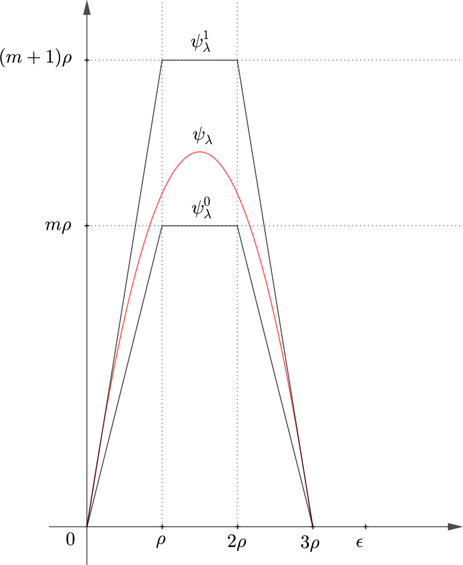
in the following way (see Figure 3):
 $$ \begin{align*} \psi_{\unicode{x3bb}}^i(r)= \left\{\!\!\begin{array}{lll} (m+i)r & \text{if }\ r \in [0,\rho] , \\ (m+i)\rho & \text{if }\ r \in (\rho, 2\rho ) ,\\ (m+i)(-r+3\rho) & \text{if }\ r \in [2\rho,3\rho]. \end{array} \right.\end{align*} $$
Bump functions
 $\psi _{\unicode{x3bb} }^0, \psi _{\unicode{x3bb} }^1$
and
 $\psi _{\unicode{x3bb} }$
(colour online).

Notice that
 $$ \begin{align*} \int_0^{\epsilon}\psi_{\unicode{x3bb}}^0(s)\,ds=2m\rho^2 < 1-\unicode{x3bb}<2(m+1)\rho^2=\int_0^{\epsilon}\psi_{\unicode{x3bb}}^1(s)\,ds. \end{align*} $$
Since
 $C^{\infty }$
functions are
 $C^0$
-dense, we can find a
 $C^{\infty }$
function
 $\psi _{\unicode{x3bb} }$
such that:
-
(1) supp
$(\psi _{\unicode{x3bb} })\subseteq [0,\epsilon ]$
; -
(2)
$\psi _{\unicode{x3bb} }^0(s) \leq \psi _{\unicode{x3bb} }(s) \leq \psi _{\unicode{x3bb} }^1(s)$
for every
$s\in [0,\epsilon ]$
; -
(3)
$\int _0^{\epsilon }\psi _{\unicode{x3bb} }(s)\,ds=1-\unicode{x3bb} $
.


Notice that point (2) implies that
 $\beta _{\unicode{x3bb} }^1(r)\leq \beta _{\unicode{x3bb} }(r)\leq \beta _{\unicode{x3bb} }^0(r)$
for every
 $r\in [0,\epsilon ]$
.
Remark 4.5. The function
 $\psi _{\unicode{x3bb} }$
(Figure 3) is not
 $C^{\infty }$
at the points
 $0$
and
 $3\rho $
. However, this can be fixed as follows. First, we can define
 $\psi _{\unicode{x3bb} }$
in the interval
 $(-\epsilon ,0)$
by symmetry using the equation
 $\psi _{\unicode{x3bb} }(t)=-\psi _{\unicode{x3bb} }(-t)$
. Then,
 $\psi _{\unicode{x3bb} }$
is
 $C^{\infty }$
at
 $0$
, and
 $\beta _{\unicode{x3bb} }$
becomes
 $C^{\infty }$
at
 $0$
(notice that
 $\beta _{\unicode{x3bb} }$
is obtained by integrating
 $\psi _{\unicode{x3bb} }$
only at the non-negative real line, so this extension to negative numbers is not a problem). To deal with the point
 $3\rho $
, we only have to take a local perturbation of
 $\psi _{\unicode{x3bb} }$
at this point to have the desired properties. Since
 $3\rho $
is far enough from 0, this can be done easily.
In the same way, we can find a suitable
 $C^{\infty }$
function
 $\psi _{\mu }$
by approximating it by two
 $C^0$
functions
 $\psi _{\mu }^1$
and
 $\psi _{\mu }^0$
by above and below, which implies that
 $\beta _{\mu }$
will be approximated by below and above by their corresponding
 $C^1$
functions
 $\beta _{\mu }^1$
and
 $\beta _{\mu }^0$
according to Lemma 4.1.
Recall that
 $2\rho ^2<\mu -1$
, then let
 $n\in {\mathbb R}^+$
be such that
 $2n\rho ^2<\mu -1<2(n+1)\rho ^2$
. Now, for
 $i=0,1$
, we define the function
 $\psi _{\mu }^i$
in the following way:
 $$ \begin{align*}\psi_{\mu}^i(r)= \left\{\!\!\begin{array}{lll} (n+i)r & \text{if }\ r \in [0,\rho], \\ (n+i)\rho & \text{if }\ r \in (\rho, 2\rho), \\ (n+i)(-r+3\rho) & \text{if }\ r \in [2\rho,3\rho]. \end{array} \right.\end{align*} $$
In the same way as above, we observe that
 $$ \begin{align*} \int_0^{\epsilon}\psi_{\mu}^0(s)\,ds=2n\rho^2<\mu-1<2(n+1)\rho^2=\int_0^{\epsilon}\psi_{\mu}^1(s)\,ds. \end{align*} $$
Since
 $C^{\infty }$
functions are
 $C^0$
-dense, we can find a
 $C^{\infty }$
function
 $\psi _{\mu }$
such that:
-
(1) supp
$(\psi _{\mu })\subseteq [0,\epsilon ]$
; -
(2)
$\psi _{\mu }^0(s) \leq \psi _{\mu }(s) \leq \psi _{\mu }^1(s)$
for every
$s\in [0,\epsilon ]$
; -
(3)
$\int _0^{\epsilon }\psi _{\mu }(s)\,ds=\mu -1$
.


Notice that point (2) implies that
 $\beta _{\mu }^1(r)\leq \beta _{\mu }(r)\leq \beta _{\mu }^0(r)$
for every
 $r\in [0,\epsilon ]$
.
Recall that we want to prove that the cones
 $\mathcal {C}^u$
are
 $Dg$
-invariant. We are going to obtained the invariance of the cones for
 $C^1$
close diffeomorphisms
 $g^0$
and
 $g^1$
defined (in the same way as g) by equation (4.1), but using the functions
 $\beta _{\unicode{x3bb} }^0$
,
 $\beta _{\mu }^0$
and
 $\beta _{\unicode{x3bb} }^1$
,
 $\beta _{\mu }^1$
, respectively, instead of
 $\beta _{\unicode{x3bb} }$
and
 $\beta _{\mu }$
. Notice that for
 $i=0,1$
, the
 $C^1$
distance between g and
 $g^i$
can be taken as small as we want.
Now, for
 $i=0,1$
, to see the cones
 $\mathcal {C}^u$
are
 $Dg^i$
-invariant, we have to prove that if
 ${(a,b)\in {\mathcal C}^u}$
, then
 $Dg^i(a,b)=(a_1,b_1)\in {\mathcal C}^u$
, and this happens if and only if
 $|a_1|\leq |b_1|$
. We will obtain this inequality by studying different cases depending on r, which is the square of the distance of the point
 $(x,y)$
to the origin.
Case 1:
 $r\in [0,\rho ]$
. By our definitions above, we have
 $$ \begin{align*}\beta_{\unicode{x3bb}}^i(r)=1-\unicode{x3bb} -(m+i)\frac{r^2}{2} \quad\text{and}\quad (\beta_{\unicode{x3bb}}^i)'(r)=-(m+i)r. \end{align*} $$
Then, we have that
 $$ \begin{align*}\unicode{x3bb}+ \beta_{\unicode{x3bb}}^i(r)+2x^2(\beta_{\unicode{x3bb}}^i) '(r)=1-(m+i)\frac{r^2}{2}-2x^2 (m+i)r \end{align*} $$
and as a consequence, we obtain that
 $a_1$
is equal to
 $$ \begin{align*}a_1 = a \bigg( 1-(m+i)\frac{r^2}{2}-2x^2 (m+i)r \bigg) + b (-2xy(m+i)r ). \end{align*} $$
Since
 $|a|\leq |b|$
, by taking the absolute value and applying the triangular inequality, we get
 $$ \begin{align*} |a_1|&\leq |b|\bigg( 1-(m+i)\frac{r^2}{2}-2x^2 (m+i)r \bigg) + |b| ( 2|xy|(m+i)r) \\ &= |b|\bigg(1 -(m+i)\frac{r}{2}( r+4x^2 -4|xy| ) \bigg) \leq |b|, \end{align*} $$
where the last inequality holds as long as
 $r+4x^2-4|xy|=5x^2+y^2-4|xy|>0$
. We claim that this is always the case: if
 $|xy|=xy$
, we have to show that
 $5x^2+y^2-4xy>0$
. By solving the second degree equation in y, we obtain that
 $$ \begin{align*}y=\frac{4x\pm \sqrt{16x^2-20x^2}}{2} \end{align*} $$
and this has no real roots. Since for
 $y=0$
we have
 $5x^2\geq 0$
, we obtain the desired inequality. The case where
 $|xy|=-xy$
is completely the same, since the discriminant in the equation above is the same. We conclude that
 $r+4x^2-4|xy|\geq 0$
and, moreover,
 $|a_1|<|b|$
if
 $r>0$
.
In the same way, we have that
 $$ \begin{align*}\beta_{\mu}^i(r)=\mu-1 - ( n+i)\frac{r^2}{2}\quad\text{and}\quad (\beta_{\mu}^i)'(r)=-(n+i)r, \end{align*} $$
and then
 $$ \begin{align*}\mu -\beta_{\mu}^i(r)-2y^2(\beta_{\mu}^i)'(r)=1+ (n+i)\frac{r^2}{2}+2y^2 (n+i )r. \end{align*} $$
We then have that
 $b_1$
is equal to
 $$ \begin{align*} b_1=a (2xy( n+i)r)+ b \bigg( 1+ (n+i)\frac{r^2}{2}+2y^2 ( n+i)r\bigg). \end{align*} $$
Since
 $|a|\leq |b|$
, taking the absolute value and by the triangular inequality, we have
 $$ \begin{align*} |b_1|&\geq |b| \bigg( 1+ (n+i)\frac{r^2}{2}+2y^2 ( n+i)r \bigg)-|b| (2|xy|( n+i )r) \\ &= |b|\bigg( 1+\frac{r}{2} (n+i) ( r+4y^2-4|xy|)\bigg) \geq |b|, \end{align*} $$
where the last inequality holds as long as
 $r+4y^2-4|xy|=x^2+5y^2-4|xy|\geq 0$
. This is exactly the same equation we solve above, and thus we conclude that
 $|b_1|\geq |b|$
and, moreover,
 $|b_1|>|b|$
if
 $r>0$
. Then, we conclude that
 $|a_1|\leq |b|\leq |b_1|$
.
Case 2:
 $r\in [\rho ,2\rho ]$
. In this case, we obtain that
 $\beta _{\unicode{x3bb} }^i$
verifies
 $$ \begin{align*}\beta_{\unicode{x3bb}}^i(r)=1-\unicode{x3bb}-(m+i)\frac{\rho^2}{2} -(m+i)\rho(r-\rho) \quad \text{and}\quad (\beta_{\unicode{x3bb}}^i)'(r)=-(m+i)\rho. \end{align*} $$
Then, we have that
 $$ \begin{align*}\unicode{x3bb}+ \beta_{\unicode{x3bb}}^i(r)+2x^2(\beta_{\unicode{x3bb}}^i)'(r)=1-(m+i)\frac{\rho^2}{2} -(m+i)\rho(r-\rho) -2x^2(m+i)\rho; \end{align*} $$
therefore,
 $a_1$
is equal to
 $$ \begin{align*}a_1 = a \bigg( 1-(m+i)\frac{\rho^2}{2} -(m+i)\rho(r-\rho) -2x^2(m+i)\rho \bigg) + b ( -2xy(m+i)\rho ). \end{align*} $$
Since
 $|a|\leq |b|$
, taking the absolute value and applying the triangular inequality, we get
 $$ \begin{align*} |a_1|&\leq |b| \bigg( 1-(m+i)\frac{\rho^2}{2} -(m+i)\rho(r-\rho) -2x^2(m+i)\rho \bigg)\\ &\quad + |b| ( 2|xy|(m+i)\rho ) \\ &= |b|\bigg( 1-(m+i)\frac{\rho^2}{2} -(m+i)\rho(r-\rho) -2x^2(m+i)\rho + 2|xy|(m+i)\rho \bigg) \\ &= |b|\bigg(1-\bigg(\frac{(m+i)\rho}{2}\bigg)\bigg( 6x^2+2y^2-4|xy|-\rho \bigg) \bigg) \leq |b|, \end{align*} $$
where the last inequality holds as long as
 $6x^2+2y^2-4|xy|-\rho \geq 0$
. Notice that
 $$ \begin{align*} 6x^2+2y^2-4|xy|-\rho=(x^2+y^2-\rho)+(5x^2+y^2-4|xy|). \end{align*} $$
The first term in the right expression is greater or equal to zero since
 $\rho \leq r$
. The second term
 $5x^2+y^2-4|xy|$
is exactly the same equation we solve in case 1.
In the same way, we have that
 $$ \begin{align*} \beta_{\mu}^i(r)=\mu-1-\frac{\rho^2}{2}(n+i)-(r-\rho)\rho (n+i)\quad\text{and}\quad (\beta_{\mu}^i)'(r)= -(n+i)\rho, \end{align*} $$
and then we obtain
 $$ \begin{align*} \mu-\beta_{\mu}^i(r)-2y^2(\beta_{\mu}^i)'(r)=1+ \frac{\rho^2}{2} (n+i) + (r-\rho)\rho(n+i)+2y^2 (n+i)\rho. \end{align*} $$
We then have that
 $b_1$
is equal to
 $$ \begin{align*} b_1=a (2xy ( n+i) \rho) + b \bigg(1+\frac{\rho^2}{2} (n+i) + (r-\rho)\rho ( n+i) + 2y^2 (n+i)\rho \bigg). \end{align*} $$
Since
 $|a|\leq |b|$
, taking the absolute value and by the triangular inequality, we have
 $$ \begin{align*} |b_1|&\geq |b|\bigg(1+\frac{\rho^2}{2} (n+i) + (r-\rho)\rho ( n+i)+2y^2 (n+i)\rho\bigg)\\ &\quad- |b| ( 2|xy|( n+i) \rho ) \\ &= |b|\bigg( 1+ \frac{\rho^2}{2}( n+i)+ (r-\rho)\rho(n+i)+2y^2(n+i)\rho-2|xy|(n+i)\rho \bigg) \\ &= |b|\bigg( 1+ \bigg(\frac{(n+i)\rho}{2}\bigg)(2x^2+6y^2-\rho-4|xy|)\bigg) \geq |b| \end{align*} $$
by the same estimates as above. Moreover, we have that
 $|b_1|>|b|$
if
 $r>0$
. Then, we conclude that
 $|a_1|\leq |b| \leq |b_1|$
.
Case 3:
 $r\in [2\rho ,3\rho ]$
. This is the simplest case, since we are far enough to zero and so we omit the calculations.
To sum up, we have proved that for
 $i=0,1$
, the cones
 $\mathcal {C}^u$
are
 $Dg^i$
-invariant. In fact, we have proved that if
 $(a,b)\in {\mathcal C}^u$
, then
 $Dg^i(a,b)=(a_1,b_1)$
verifies
 $|a_1|\leq |b_1|$
. Now, just notice that the inequality
 $|a_1|\leq |b_1|$
depends on the values of the entries of
 $Dg^i$
. Since the entries of
 $Dg$
are bounded by above and below by the entries of
 $Dg^i$
, by taking suitable triangular inequalities, it is easy to see that the inequality
 $|a_1|\leq |b_1|$
also holds for
 $Dg$
, proving that the cones
 $\mathcal {C}^u$
are also
 $Dg$
-invariant.
Now, if we take the norm
 $\lVert (a,b)\rVert _1:=\max \{|a|,|b|\}$
in
 ${\mathbb R}^2$
, we have that vectors in
 ${\mathcal C}^u$
are expanded for the future: if
 $v=(a,b)\in {\mathcal C}^u$
, then
 $|a|\leq |b|$
and thus
 $\lVert v\rVert _1=|b|$
. Since
 $Dg(v)=(a_1,b_1) \in {\mathcal C}^u$
, this implies that
 $\lVert Dg(v)\rVert _1=|b_1|$
and we have just proved that
 $|b|\leq |b_1|$
. This implies that
 $\lVert Dg(v)\rVert _1 \geq \lVert v\rVert _1$
and, moreover,
 $\lVert Dg_{(x,y)}(v)\rVert _1> \lVert v\rVert _1$
if
 $(x,y)\neq (0,0)$
.
Next, we define the Lyapunov function
 $V:{\mathbb R}^2\times {\mathbb R}^2\to {\mathbb R}$
given by
 $$ \begin{align*} V((x_1,y_1),(x_2,y_2))=(y_1-y_2)^2-(x_1-x_2)^2. \end{align*} $$
Let
 $P=(x_1,y_1)$
and
 $Q=(x_2,y_2)$
be two different points in
 ${\mathbb R}^2$
. Then,
 $V(P,Q)=(y_1-y_2)^2-(x_1-x_2)^2$
. Let us denote
 $g(P)=(x_1',y_1')$
and
 $g(Q)=(x_2',y_2')$
, then
 $V(g(P),g(Q))=(y_1'-y_2')^2-(x_1'-x_2')^2$
.
Now, take the function
 $\varphi :[0,1]\to {\mathbb R}$
given by
 $\varphi (t)=\Pi _2(g(tP+(1-t)Q))$
, where
 $\Pi _2:{\mathbb R}^2\to {\mathbb R}$
is the projection in the second coordinate. Notice that
 $\varphi (0)=y_2'$
,
 $\varphi (1)=y_1'$
and
 $\varphi $
is differentiable. Then, by the mean value theorem, we have
 $$ \begin{align*}|y_2'-y_1'|&=|\varphi(0)-\varphi(1)|=|\varphi'(t_0)|=|\Pi_2 \circ Dg_{z_0}(P-Q)|\\&=|Dg_{z_0}(0,y_1-y_2)|>|y_1-y_2| \end{align*} $$
for some
 $z_0$
. In the same way, we get that
 $|x_1'-x_2'|<|x_1-x_2|$
, and this implies that
 $\Delta V(P,Q)>0$
. This ends the proof of the lemma.
Corollary 4.6. Let
 $A\in \mathrm {SL}(2,{\mathbb Z})$
be a hyperbolic matrix and take
 ${\varepsilon }>0$
sufficiently small. Then, there is a diffeomorphism
 $g:{\mathbb T}^2 \to {\mathbb T}^2$
such that:
-
•
$g(x,y)=A(x,y)$
for every
$(x,y) \in B(0,{\varepsilon })^c$
; -
•
$Dg_{(0,0)}=\mathrm {Id}$
; -
• g belongs to the
$C^1$
boundary of Anosov diffeomorphisms; -
• g is expansive and conjugated to A.


Proof. Let
 $A\in \mathrm {SL}(2,{\mathbb Z})$
be as in the hypothesis and suppose the eigenvalues of A are
 $\unicode{x3bb} $
and
 $\mu $
with
 $0<\unicode{x3bb} <1<\mu $
. Let
 $E^s$
be the eigenspace associated to
 $\unicode{x3bb} $
, and let
 $E^u$
be the eigenspace associated to
 $\mu $
. Then, we have that
 ${\mathbb R}^2=E^s\oplus E^u$
. Now, for
 ${\varepsilon }>0$
and identifying
 ${\mathbb R}^2$
with
 $E^s\oplus E^u$
, we take the map
 $g:{\mathbb R}^2\to {\mathbb R}^2$
given by Lemma 4.4. We can take
 $\epsilon $
small enough so we can send the map g to the quotient
 ${\mathbb T}^2={\mathbb R}^2/{\mathbb Z}^2$
(notice that we are making an abuse of notation between g and its lift to
 ${\mathbb R}^2$
).
We know that the map g has a Lyapunov function
 $V:{\mathbb R}^2\times {\mathbb R}^2\to {\mathbb R}$
given by
 $$ \begin{align*} V((x_1,y_1),(x_2,y_2))=(y_1-y_2)^2-(x_1-x_2)^2, \end{align*} $$
which verifies that
 $\Delta V((x_1,y_1),(x_2,y_2))>0$
for every pair of different (and sufficiently close) points
 $(x_1,y_1),(x_2,y_2) \in {\mathbb R}^2$
. Then, by Proposition 4.3, the map g is expansive. Notice that we are only interested in what happens in a fundamental domain, so the non-compactness of
 ${\mathbb R}^2$
is not a problem.
Finally, since g fails to be hyperbolic only at
 $(0,0)$
, we know that g is in the
 $C^1$
boundary of Anosov diffeomorphisms. Then, by [Reference Lewowicz13, Corollary 6.2], g is conjugated to A. Moreover, this implies g is infinite expansive in
 ${\mathbb R}^2$
and, in particular, the semiconjugacy
 $H_g$
is in fact injective and
 $\Lambda (g)=0$
.
Now that we have the map
 $g:{\mathbb R}^2\to {\mathbb R}^2$
constructed in Lemma 4.4, we can build a partially hyperbolic example in
 ${\mathbb T}^4$
with a centre leaf which behaves exactly like g.
Lemma 4.7. Let
 $A\in \mathrm {SL}(4,{\mathbb Z})$
be a matrix with four eigenvalues
 $\unicode{x3bb} ^{ss},\unicode{x3bb} ,\mu ,\mu ^{uu}$
such that
 $ 0<\unicode{x3bb} ^{ss}<\unicode{x3bb} <1<\mu <\mu ^{uu}$
and take
 ${\varepsilon }>0$
. Then, there is a partially hyperbolic diffeomorphism
 $f:{\mathbb T}^4\to {\mathbb T}^4$
with a splitting of the form
 ${\mathbb R}^4=E^{ss}_f \oplus E^c_f \oplus E^{uu}_f$
, such that
 $\dim E^c_f=2$
, which verifies the following:
-
•
$f(x)=Ax$
for every
$B(0,{\varepsilon })^c$
; -
• f is expansive and conjugated to A;
-
•
$Df_0|_{E^c_f}=\mathrm {Id}$
.


Proof. Let
 $A\in \mathrm {SL}(4,{\mathbb Z})$
be a matrix with four eigenvalues
 $\unicode{x3bb} ^{ss},\unicode{x3bb} ,\mu ,\mu ^{uu}$
such that
 $$ \begin{align*} 0<\unicode{x3bb}^{ss}<\unicode{x3bb}<1<\mu<\mu^{uu}. \end{align*} $$
We can assume that in the basis given by the eigenspaces associated to the eigenvalues, we have that
 $A(x,y,z,t)=(\unicode{x3bb} x, \mu y, \unicode{x3bb} ^{ss}z,\mu ^{uu}t)$
. Take the same functions
 $\beta _{\unicode{x3bb} }$
and
 $\beta _{\mu }$
as in Lemma 4.4 and define the map
 $f:{\mathbb R}^4\to {\mathbb R}^4$
by
 $$ \begin{align*}f(x,y,z,t)=(\unicode{x3bb} x,\mu y, \unicode{x3bb}^{ss} z, \mu^{uu} t) + \rho(w)(\beta_{\unicode{x3bb}}(r)x,-\beta_{\mu}(r)y,0,0), \end{align*} $$
where
 $\rho $
is a bump function supported in
 $[0,{\varepsilon }]$
and
 $w=z^2+t^2$
. We can take
 $\epsilon $
small enough so we can send the map f to the quotient
 ${\mathbb T}^4={\mathbb R}^4/{\mathbb Z}^4$
.
If
 $\lVert (x,y,z,t)\rVert \geq {\varepsilon }$
, we have that
 $f=A$
. For points with
 $\lVert (x,y,z,t)\rVert < {\varepsilon }$
, the differential of f at a point
 $(x,y,z,t)$
is
 $$ \begin{align*} \begin{bmatrix} \unicode{x3bb} +\rho(w) ( \beta_{\unicode{x3bb}}(r) +2x^2 \beta_{\unicode{x3bb}}'(r)) & \rho(w) (2xy\beta_{\unicode{x3bb}}'(r)) &2xz\rho'(w)\beta_{\unicode{x3bb}}(r) & 2tz\rho'(w)\beta_{\unicode{x3bb}}(r) \\ -\rho(w) (2xy\beta_{\mu}'(r)) & \mu -\rho(w)( \beta_{\mu}(r)-2y^2 \beta_{\mu}'(r) ) &-2yz\rho'(w)\beta_{\mu}(r) & 2yt\rho'(w)\beta_{\mu}(r) \\ 0 & 0 & \unicode{x3bb}^{ss} & 0 \\ 0 & 0 & 0 & \mu^{uu} \end{bmatrix}\!. \end{align*} $$
In this case, the subspace
 $E^c_f=\{(x,y,0,0)\}$
is
 $Df$
invariant, and it is quite direct to see that
 $Df|_{E^c_f}$
is basically
 $Dg$
like above (we have to deal with the function
 $\rho $
, but this is not a problem). In particular, we have that
 $$ \begin{align*} Df_0= \begin{bmatrix} 1 & 0 & 0 & 0 \\ 0 & 1 & 0 & 0 \\ 0 & 0 & \unicode{x3bb}^{ss} & 0 \\ 0 & 0 & 0 & \mu^{uu} \end{bmatrix}. \end{align*} $$
The strong bundles are not going to be the canonical ones, but if we ask for the strong eigenvalues
 $\unicode{x3bb} ^{ss}$
and
 $\mu ^{uu}$
to be sufficiently far away from 1 (and we can do this by iterating the matrix), the same strong cones for the matrix A are going to be
 $Df$
-invariant.
Finally, in the same way as in Lemma 4.4 and Corollary 4.6, by taking the Lyapunov function
 $V:{\mathbb R}^4 \times {\mathbb R}^4 \to {\mathbb R}$
given by
 $$ \begin{align*} V((x_1,y_1,z_1,t_1),(x_2,y_2,z_2,t_2))=(y_1-y_2)^2 -(x_1-x_2)^2 + (t_1-t_2)^2-(z_1-z_2)^2, \end{align*} $$
it is easy to see that
 $\Delta V((x_1,y_1,z_1,t_1),(x_2,y_2,z_2,t_2))>0$
for every pair of different (and sufficiently close) points
 $(x_1,y_1,z_1,t_1),(x_2,y_2,z_2,t_2) \in {\mathbb R}^4$
. Then, by Proposition 4.3, we conclude that
 $f:{\mathbb T}^4\to {\mathbb T}^4$
is an expansive diffeomorphism. Moreover, f is in the
 $C^1$
boundary of Anosov diffeomorphisms and by [Reference Lewowicz13, Corollary 6.2], f is conjugated to A (which implies
 $\Lambda (f)=0$
).
Remark 4.8. The construction in Lemma 4.7 can be made with no restriction on the dimensions of the strong subbundles (which were one-dimensional in the example above). Indeed, the construction only uses the local isotopy in dimension 2 we made in Lemma 4.4 and the domination of the external strong subbundles.
4.1.2 Higher dimensional centre bundle
We now deal with the case where the centre bundle has dimension bigger than 2. We are going to treat the case where the centre bundle
 $E^c_A$
is contractive (every centre eigenvalue has modulus smaller than 1) since it is the only case that matters for our purposes. The case where the centre bundle
 $E^c_A$
is expanding (every centre eigenvalue has modulus bigger than 1) is completely analogous. We remark that the proof works as well for the case where the centre is two-dimensional.
In Lemma 4.9, we construct the example in
 ${\mathbb R}^k$
and then in Lemma 4.10, we insert the example as the centre leaf of a partially hyperbolic diffeomorphism like we did before.
Lemma 4.9. Let
 $A\in \mathrm {M}_{k\times k}({\mathbb Z})$
be a diagonal matrix with k eigenvalues such that

Then for every
 ${\varepsilon }>0$
, there is a diffeomorphism
 $g:{\mathbb R}^k\to {\mathbb R}^k$
such that:
-
•
$g(x)=Ax$
for every
$x\in B(0,{\varepsilon })^c$
; -
•
$\lVert Dg_x\rVert <1$
for every
$x\neq 0$
; -
•
$Dg_0=\mathrm {Id}$
.


Proof. Take a matrix
 $A\in M_{k\times k}({\mathbb Z})$
as above. Then the eigenvalues of A verify that

Fix
 ${\varepsilon }>0$
small and take
 $\unicode{x3bb} $
such that
 $\unicode{x3bb} _k < \unicode{x3bb} < 1$
. In particular,
 $\unicode{x3bb}> \unicode{x3bb} _j$
for every
 $j=1,\ldots ,k$
. Now take a number
 $c\in (0,{\varepsilon })$
such that
 $c< ({1-\unicode{x3bb} })/({k(\unicode{x3bb} -\unicode{x3bb} _1)})$
. Now, for this
 $c>0$
, take the function
 $\beta $
given by Lemma 4.1 for
 $b=1$
. In particular, the function
 $\beta $
verifies:
-
•
$\beta $
is
$C^{\infty }$
and decreasing; -
•
$\beta $
is supported in
$[0,{\varepsilon }]$
; -
•
$\beta (0)=1$
.


Moreover, we can ask for
 $\beta $
to be equal to 1 in a small interval
 $[0,\delta ]$
. Now, we can define the map
 $g_1:{\mathbb R}^k \to {\mathbb R}^k$
by

where
 $r=x_1^2+\cdots +x_k^2$
. Since supp
 $(\beta )\subseteq [0,{\varepsilon }]$
, we have that if
 $\lVert x\rVert>{\varepsilon }$
, then
 $g_1=A$
. The differential of
 $g_1$
in a point x is

where
 $M(x)$
is the matrix given by

In particular, since
 $\beta (0)=1$
, we have that
 $D(g_1)_0=A+\beta (0)(\unicode{x3bb} \mathrm {Id} -A)+M(0)=\unicode{x3bb} \mathrm {Id}$
. Now, take a point
 $x\in {\mathbb R}^k$
and a vector
 $v\in {\mathbb R}^k$
, then we have that
 $$ \begin{align*}D(g_1)_x(v)=Av+\beta(r)(\unicode{x3bb} \mathrm{Id}-A)v+M(x)v. \end{align*} $$
Assume the vector v is equal to
 $v=(a,\ldots ,a)\in {\mathbb R}^k$
for a given
 $a\in {\mathbb R}$
and denote
 $D(g_1)_x(v)=(a_1,\ldots ,a_k)$
. If we prove that
 $|a_j|<|a|$
for every
 $j=1,\ldots ,k$
, we obtain that
 $D(g_1)_x$
is a contraction (by taking the norm of the maximum). Let us take a look at the first coordinate
 $a_1$
:

By taking the absolute value and applying the triangular inequality, we obtain

Notice that
 $0\leq (x_i+x_j)^2=x_i^2+x_j^2+2x_ix_j$
and this implies
 $2|x_ix_j|\leq x_i^2+x_j^2\leq r$
. Now, recall that
 $|\beta '(r)|\leq ({c}/{r}) < ({1-\unicode{x3bb} })/({k(\unicode{x3bb} -\unicode{x3bb} _1)r}) $
and, in particular, we have that

This implies that

Since
 $\beta $
is a decreasing function, we have that
 $1=\beta (0)\geq \beta (r)$
and then

The exact same calculation shows that
 $|a_j|<|a|$
for every
 $j=1,\ldots ,k$
. This shows that
 $D(g_1)_x$
is a contraction (for the norm of the maximum) for every
 $x\in {\mathbb R}^k$
and, in particular,
 $g_1$
is expansive. Notice that since
 $\beta (r)=1$
for every
 $r\in [0,\delta ]$
, we have that
 $g_1(x)=\unicode{x3bb} x$
for every
 $x\in B(0,\delta )$
. Now, take the function
 $h:{\mathbb R}^k\to {\mathbb R}^k$
given by
 $h(x)=(1-r)x$
, where
 $r=\lVert x\rVert ^2$
and consider a bump function
 $\rho :[0,+\infty ) \to {\mathbb R}$
such that:
-
•
$\rho (t)=1$
for every
$t\in [0,\delta /2]$
; -
•
$\rho (t)=0$
for every
$t\geq \delta $
.


Now, we define
 $g:{\mathbb R}^k\to {\mathbb R}^k$
given by the equation:
 $$ \begin{align*} g(x)=\rho(r)h(x)+(1-\rho(r))g_1(x), \end{align*} $$
where
 $r=\lVert x\rVert ^2$
. The first observation is that if
 $\lVert x\rVert \geq \delta $
, then
 $g(x)=g_1(x)=Ax$
. However, if
 $r=\lVert x\rVert ^2\leq \delta $
, then we have that
 $g_1(x)=\unicode{x3bb} x$
and, therefore,
 $$ \begin{align*}g(x)=\rho(r)h(x)+(1-\rho(r))\unicode{x3bb} x=[\rho(r)(1-r)+(1-\rho(r))\unicode{x3bb}]x\end{align*} $$
and the function g is radial. Denote
 $\alpha (r):=\rho (r)(1-r)+(1-\rho (r))\unicode{x3bb} $
, then it is direct to see that
 $$ \begin{align*} \alpha(r)=\rho(r)(1-r)+(1-\rho(r))\unicode{x3bb}=\rho(r)(1-r-\unicode{x3bb})+\unicode{x3bb} \leq 1-r.\end{align*} $$
As a result, g sends every sphere of radius R to a sphere of radius
 $\alpha (R)R$
which is strictly smaller than R. This implies that
 $Dg_x$
is a contraction for every
 $x\in B(0,\delta )$
. To see this, just notice that given
 $x\in {\mathbb R}^k$
, we have that
 $T_x{\mathbb R}^k=T_x S_{\lVert x\rVert }+ \langle x \rangle $
, where
 $S_{\lVert x\rVert }$
is the sphere centred at 0 of radius
 $\lVert x\rVert $
. The same happens with
 $g(x)$
, that is,
 $T_{g(x)}{\mathbb R}^k=T_{g(x)} S_{\alpha (\lVert x\rVert )\lVert x\rVert }+ \langle x \rangle $
and the differential of g at x restricted to this subspace is exactly
 $$ \begin{align*}Dg_x|_{T_xS_{\lVert x\rVert}}=\alpha(\lVert x\rVert)\mathrm{Id},\end{align*} $$
which is a contraction. The other direction
 $\langle x \rangle $
is exactly the same, and, therefore,
 $Dg_x$
is a contraction. To finish the proof, just observe that if
 $r=\lVert x\rVert ^2<\delta /2$
, we have that
 $g(x)=(1-r)x$
and, in particular,
 $Dg_0=\mathrm {Id}$
.
Now, by applying the same trick as in Lemma 4.7 (with a suitable bump function), we can embed the example above as the centre leaf of a higher dimensional manifold. We thus obtain the following result whose proof we omit since it is exactly the same as that of the lemma we just mentioned.
Lemma 4.10. Let
 $A\in \mathrm {SL}(n,{\mathbb Z})$
be a symmetric matrix with a splitting of the form
 ${\mathbb R}^n=E^{ss}_A\oplus E^c_A \oplus E^{uu}_A$
such that
 $\dim E^c_A=k$
and
 $E^c_A$
is the eigenspace associated to the eigenvalues
 $0<\unicode{x3bb} _1\leq \cdots \leq \unicode{x3bb} _k<1$
. Then, for every
 ${\varepsilon }>0$
small, there is
 $f\in {\mathcal {PH}}_A({\mathbb T}^n)$
such that:
-
•
$f(x)=Ax$
for every
$x\in B(0,{\varepsilon })^c$
; -
• f is expansive and conjugated to A;
-
•
$Df_0|_{E^c_f}=\mathrm {Id}.$


We now proceed to finish the proof of Theorem A. We begin with the case where
 $n=4$
, since it is quite direct for our previous results and illustrates the general ideas. We then prove the general case.
4.2 Proof for case
$n=4$

Take a matrix
 $A\in \mathrm {SL}(4,{\mathbb Z})$
with four eigenvalues
 $\unicode{x3bb} ^{ss},\unicode{x3bb} ,\mu ,\mu ^{uu}$
such that
 $$ \begin{align*} 0<\unicode{x3bb}^{ss}<\unicode{x3bb}<1<\mu<\mu^{uu}.\end{align*} $$
This induces a splitting of the form
 ${\mathbb R}^4=E^{ss}\oplus E^{ws}\oplus E^{wu}\oplus E^{uu}$
and we take the centre bundle as
 $E^c=E^{ws}\oplus E^{wu}$
. We can assume that in the basis given by the eigenspaces associated to the eigenvalues, we have that
 $$ \begin{align*}A(x,y,z,t)=(\unicode{x3bb} x, \mu y, \unicode{x3bb}^{ss}z,\mu^{uu}t).\end{align*} $$
Moreover, we can assume that the linear Anosov A has four different fixed points: Fix
 $(A)=\{p_0,p_1,p_2,p_3\}$
(we are making an abuse of notation here, by calling A, instead of
 $f_A$
, the induced map in the torus). We just have to iterate the matrix a few times to have four different fixed points.
Now, notice that the procedure made in §4.1 works as well. First, for every fixed point
 $p_j$
(with
 $j=0,1,2$
), take a small neighbourhood
 $U_j$
(notice that we are not going to perturb
 $p_3$
since it already has index 2). We can take them small enough to be disjoint. Second, just notice that the isotopy procedure we made in Lemma 4.4 is only local and, therefore, it can be applied in different disjoint neighbourhoods. Hence, the same proof as in Lemma 4.7 shows that we can make an isotopy whose support is contained in
 $U_0 \cup U_1 \cup U_2$
to get a partially hyperbolic diffeomorphism
 $f_1: {\mathbb T}^4\to {\mathbb T}^4$
such that:
-
•
$f_1(x)=Ax$
for every
$x\in (U_0 \cup U_1 \cup U_2)^c$
; -
•
$f_1$
is hyperbolic outside
$Fix(f_1)=\{p_0,p_1,p_2\}$
; -
•
$D(f_1)_{p_j}|_{E^c_{f_1}(p_j)}=\mathrm {Id}$
for
$j=0,1,2$
.


Since
 $f_1$
is hyperbolic outside Fix
 $(f_1)=\{p_0,p_1,p_2\}$
, once again, we can find an appropriate Lyapunov function to apply Proposition 4.3 and get that
 $f_1$
is expansive. Since
 $f_1$
is in the
 $C^1$
boundary of Anosov diffeomorphisms, by [Reference Lewowicz13, Corollary 6.2], we have that
 $f_1$
is conjugated to A, which implies
 $\Lambda (f_1)=0$
.
The first point shows that
 $f_1$
is an SH-saddle of index (1,1). To see this, we just have to observe that the same proof of Lemma 3.1 shows that
 $f_1$
has the SH-saddle property as well. In that proof, the only property we use is the fact that, for a point p outside U and given a small
 $\delta>0$
, there is always a point
 $p_1$
such that
 $$ \begin{align*}{\mathcal W}^{uu}_{f_1}(p_1,\delta)\subset f_1({\mathcal W}^{uu}_{f_1}(p,\delta))\cap (U^c)\end{align*} $$
and by an induction argument, we find a point whose forward orbit never meets U, and the same happens for the past. Hence,
 $f_1$
is the SH-saddle of index (1,1). By the same arguments, by taking the strong bundles
 $E^{ss}$
and
 $E^{uu}$
sufficiently contractive and expanding, and taking the neighbourhoods
 $U_j$
sufficiently small, we also have this property, that is, for every point p outside
 $U_0\cup U_1\cup U_2$
, and given a small
 $\delta>0$
, there is always a point
 $p_1$
such that
 $$ \begin{align*}{\mathcal W}^{uu}_{f_1}(p_1,\delta)\subset f_1({\mathcal W}^{uu}_{f_1}(p,\delta))\cap (U_0\cup U_1\cup U_2)^c.\end{align*} $$
Then, we can find a point that never meets
 $U_0\cup U_1\cup U_2$
for the future, and the same for the past. In short,
 $f_1$
has the (1,1) SH-saddle property.
Now, since
 $f_1$
is the SH-saddle, we have that
 $\rho (f_1)>0$
and, by expansiveness, we also have
 $\Lambda (f_1)=0$
. Then, a direct application of Theorem 3.8 shows that
 $f_1$
is
 $C^1$
robustly transitive. Let us call
 ${\mathcal U}_1$
to the
 $C^1$
neighbourhood of
 $f_1$
such that every
 $h\in {\mathcal U}_1$
is transitive.
To end the proof of the theorem, we are going to change the indexes of the fixed points
 $p_0$
and
 $p_1$
, and put a complex eigenvalue in
 $p_2$
. First, take the two matrices
 $B_0$
and
 $B_1$
given by
 $$ \begin{align*} B_0= \begin{bmatrix} 1-\eta & 0 & 0 & 0 \\ 0 & 1-\eta & 0 & 0 \\ 0 & 0 & \unicode{x3bb}^{ss} & 0 \\ 0 & 0 & 0 & \mu^{uu} \end{bmatrix}, \quad B_1= \begin{bmatrix} 1+\eta & 0 & 0 & 0 \\ 0 & 1+\eta & 0 & 0 \\ 0 & 0 & \unicode{x3bb}^{ss} & 0 \\ 0 & 0 & 0 & \mu^{uu} \end{bmatrix}. \end{align*} $$
Then, for
 $\eta $
sufficiently small, we have that the matrices
 $B_0$
and
 $B_1$
are
 ${\varepsilon }$
close to
 $D(f_1)_{p_0}$
and
 $D(f_1)_{p_1}$
, respectively. Now, to mix the two centre subbundles, take the matrix
 $B_2$
with the form:
 $$ \begin{align*} B_2= \begin{bmatrix} a & b & 0 & 0 \\ -b & a & 0 & 0 \\ 0 & 0 & \unicode{x3bb}^{ss} & 0 \\ 0 & 0 & 0 & \mu^{uu} \end{bmatrix}, \end{align*} $$
where
 $a\pm ib$
are the complex eigenvalues of
 $B_2$
. It is possible to take a and b such that a is close to 1, b is close to 0 (the modulus of
 $a\pm ib$
can be smaller, bigger or equal to 1 for our purposes). For suitable values of a and b, we can assure that
 $B_2$
is
 ${\varepsilon }$
close to
 $D(f_1)_{p_2}$
. Then, by Franks lemma [Reference Franks10], there is a diffeomorphism
 $f\in {\mathcal U}_1$
such that:
-
•
$f(x)=f_1(x)$
for every
$x\in (U_0 \cup U_1 \cup U_2)^c$
; -
•
$f(p_j)=f_1(p_j)=p_j$
for
$j=0,1,2$
; -
•
$Df_{p_j}=B_j$
for
$j=0,1,2$
.


In particular, index
 $(p_0)=3$
and index
 $(p_1)=1$
(recall that index
 $(p_3)=2$
). Since
 $Df_{p_2}$
has a centre complex eigenvalue, the centre bundle of f cannot be decomposed into two one-dimensional subbundles. To sum up, the map
 $f:{\mathbb T}^4 \to {\mathbb T}^4$
is a
 $C^1$
robustly transitive derived from Anosov diffeomorphism, and verifies all the properties of Theorem A.

4.3 Proof of the general case
For the proof of the general case, we proceed like we did above. Let
 $A\in \mathrm {SL}(n,{\mathbb Z})$
be a hyperbolic symmetric matrix with a splitting of the form:
 $$ \begin{align*} {\mathbb R}^n=E^{ss}_A\oplus E^{ws}_A \oplus E^{wu}_A \oplus E^{uu}_A, \end{align*} $$
where we take
 $E^c_A:=E^{ws}_A \oplus E^{wu}_A$
as the centre bundle. Since the matrix A is symmetric, we know the subbundles
 $E^{ws}_A$
and
 $E^{wu}_A$
can be decomposed into one-dimensional subbundles, that is,
 $$ \begin{align*} {\mathbb R}^n=E^{ss}_A\oplus E^{ws}_1\oplus \cdots \oplus E^{ws}_m \oplus E^{wu}_1 \oplus \cdots \oplus E^{wu}_l \oplus E^{uu}_A, \end{align*} $$
where
 $E^{w*}_j$
is the eigenspace associated to the eigenvalue
 $\unicode{x3bb} ^{*}_j$
for
 $*=s,u$
. In particular, the eigenvalues verify
 $$ \begin{align*}\unicode{x3bb}^s_1\leq \cdots \leq \unicode{x3bb}^s_m<1<\unicode{x3bb}^u_1 \leq \cdots \leq \unicode{x3bb}^u_l.\end{align*} $$
In short,
 $m=\dim E^{ws}_A$
,
 $l=\dim E^{wu}_A$
and
 $k=\dim E^c_A=m+l$
.
Notice that 0 is a fixed point of A and index
 $(0)=\dim E^{ss}_A+m$
. Now, by iterating the matrix if necessary, we can take
 $k=m+l$
different fixed points of A (here we are making an abuse of notation once again), Fix
 $(A)=\{p_1,\ldots , p_m,q_1,\ldots ,q_l\}$
. For every
 $j=1,\ldots ,m$
, take a neighbourhood
 $U_j$
of
 $p_j$
, and for every
 $j=1,\ldots ,l$
, take a neighbourhood
 $V_j$
of
 $q_j$
. We can assume that they are small enough to be disjoint.
Like before, we proceed like in §4.1. Notice that the isotopies we made in that subsection were only local. Therefore, a direct application of Lemma 4.10 implies that there is a partially hyperbolic diffeomorphism
 $g:{\mathbb T}^n\to {\mathbb T}^n$
with a splitting of the form
 $$ \begin{align*}T{\mathbb T}^n=E^{ss}_g\oplus E^{ws}_g\oplus E^{wu}_g \oplus E^{uu}_g,\end{align*} $$
where
 $\dim E^{*}_A=\dim E^{*}_g$
for
 $*=ss,ws,wu,uu$
, and moreover:
-
•
$g(x)=Ax$
for every
$x\in ( U_1 \cup \cdots \cup U_m \cup V_1 \cup \cdots \cup V_l)^c$
; -
• g is hyperbolic outside Fix
$\{g\}$
; -
•
$Dg_{p_j}|_{E^{ws}_g}=\mathrm {Id}$
for every
$j=1,\ldots ,m$
; -
•
$Dg_{q_j}|_{E^{wu}_g}=\mathrm {Id}$
for every
$j=1,\ldots ,l$
.


Once again, by taking the neighbourhoods
 $U_i$
and
 $V_j$
sufficiently small, the same argument in Lemma 3.1 implies g has the SH-saddle property of index
 $(m,l)$
. The second point above says that g is expansive and in the
 $C^1$
boundary of Anosov diffeomorphisms. Then, by [Reference Lewowicz13, Corollary 6.2], g is conjugated to A, which implies
 $\Lambda (g)=0$
. Then, by Theorem 3.8 (or Corollary 3.10), we have that g is
 $C^1$
robustly transitive. Let
 ${\mathcal U}$
be the
 $C^1$
neighbourhood of g such that every
 $h\in {\mathcal U}$
is transitive, and let
 ${\varepsilon }>0$
be such that
 $B_{C^1}(g,{\varepsilon })\subset {\mathcal U}$
.
Now, for this
 ${\varepsilon }$
, take m hyperbolic matrices
 $B_1,\ldots ,B_m$
which are
 ${\varepsilon }$
close to
 $Dg_{p_1},\ldots , Dg_{p_m}$
, and such that index
 $(B_j)=\dim E^{ss}_A+j$
. Notice that we can always have these matrices since
 $Dg_{p_j}|_{E^{ws}_g}=\mathrm {Id}$
for every
 $j=1,\ldots ,m$
. In the same way, we can take l hyperbolic matrices
 $C_1,\ldots ,C_l$
which are
 ${\varepsilon }$
close to
 $Dg_{q_1},\ldots , Dg_{q_l}$
, and such that index
 $(C_j)=\dim E^{ss}_A+m+j$
.
By applying Franks lemma [Reference Franks10] once again, we know there is a partially hyperbolic diffeomorphism
 $f \in {\mathcal U} \cap {\mathcal {PH}}_A({\mathbb T}^n)$
such that:
-
•
$f(x)=g(x)=Ax$
for every
$x\in ( U_1 \cup \cdots \cup U_m \cup V_1 \cup \cdots \cup V_l)^c$
; -
•
$f(p_j)=p_j$
for every
$j=1,\ldots ,m$
; -
•
$f(q_j)=q_j$
for every
$j=1,\ldots ,l$
; -
•
$Df_{p_j}=B_j$
for every
$j=1,\ldots ,m$
; -
•
$Df_{q_j}=C_j$
for every
$j=1,\ldots ,l$
.


In particular, we have
 $k+1$
fixed points (we are including 0 here) with indexes going from
 $\dim E^{ss}_A$
to
 $\dim E^{ss}_A+k$
.
To end the proof, we have to mix the centre subbundles
 $E^{ws}_m$
and
 $E^{wu}_1$
. To do this, we just have to take another different fixed point p and apply the same isotopy as in Lemma 4.4. This way, the splitting of f is not coherent with the hyperbolic splitting of A. If we want to make the entire centre undecomposable, we can take extra fixed points and make suitable local perturbations by adding complex eigenvalues. We thus obtain our example and we finish the proof of Theorem A.
4.4 Other kinds of examples
In this subsection, we are going to present two additional examples of
 $C^1$
robustly transitive partially hyperbolic diffeomorphisms. These examples are in a sense similar to those we saw in Theorem A but with a different flavour.
We begin by introducing an example which originally appeared in [Reference Lewowicz13] (see also [Reference Cerminara and Lewowicz7]) that will be used in the construction of both
 $C^1$
robustly transitive partially hyperbolic diffeomorphisms.
4.4.1 Example 0
Let A be the hyperbolic matrix
 $A=\begin {bmatrix} 2 & 1 \\ 1 & 1 \end {bmatrix}.$
Take
 $c\in [0,1]$
and consider the family of diffeomorphisms
 $f_c:{\mathbb T}^2\to {\mathbb T}^2$
given by
 $$ \begin{align*} f_c(x,y) =\bigg(2x+y-\frac{c}{2\pi}\sin(2\pi x),\,x+y-\frac{c}{2\pi}\sin(2\pi x)\bigg). \end{align*} $$
The differential of
 $f_c$
at a point
 $(x,y)$
is equal to
 $$ \begin{align*}Df_c=\begin{bmatrix} 2-c\cos(2\pi x) & 1 \\ 1-c\cos(2\pi x) & 1 \end{bmatrix}. \end{align*} $$
Notice that
 $det(Df_c)=1$
for every
 $c\in [0,1]$
and every
 $(x,y)\in {\mathbb T}^2$
; therefore,
 $f_c$
is a conservative diffeomorphism for every
 $c\in [0,1]$
. We also observe that the trace
 $tr(Df_c)=3-c\cos (2\pi x)>2$
if
 $c<1$
, which implies
 $f_c$
is Anosov (notice in particular that
 $f_0=A$
) and by the structural stability of Anosov diffeomorphisms,
 $f_c$
is conjugated to A.
When
 $c=1$
, the map
 $f_1$
is not uniformly hyperbolic since for
 $x=0$
, we have
 $$ \begin{align} Df_1=\begin{bmatrix} 1 & 1 \\ 0 & 1 \end{bmatrix} \end{align} $$
and therefore every point of the form
 $(0,y)$
has a non-hyperbolic differential and, moreover, does not admit any invariant subbundle. For points
 $(x,y)$
with
 $x\neq 0$
,
 $Df_1$
is a hyperbolic matrix since the trace is bigger than 2.
To sum up,
 $f_1$
is a conservative non-Anosov diffeomorphism on
 ${\mathbb T}^2$
. Moreover, by taking the Lyapunov function
 $V:{\mathbb R}^2\times {\mathbb R}^2 \to {\mathbb R}$
given by
 $$ \begin{align*} V((x_1,y_1),(x_2,y_2))=-(y_2-y_1)((y_2-x_2)-(y_1-x_1)), \end{align*} $$
it is easy to see that
 $$ \begin{align*}\Delta V((x_1,y_1),(x_2,y_2))=(x_2-x_1)^2+(y_2-y_1)^2-(x_2-x_1) \bigg( \frac{\sin (2\pi x_2)-\sin (2\pi x_1)}{2\pi} \bigg), \end{align*} $$
which is positive by the mean value theorem, except perhaps at finite points. By taking
 ${\gamma>0}$
sufficiently small (to remove these finite points), we have that
 $\Delta V((x_1,y_1),(x_2,y_2))>0$
if
 $0<d((x_1,y_1),(x_2,y_2))\leq \gamma $
and by Proposition 4.3, we know
 $f_1$
is
 $\gamma $
-expansive.
Finally, notice that if
 $c\to 1$
, then
 $f_c \to f_1$
in the
 $C^1$
topology, and then by [Reference Lewowicz13, Corollary 6.2], we have that
 $f_1$
is conjugated to
 $f_c$
for any c sufficiently close to 1. Since
 $f_c$
is conjugated to A for any
 $c<1$
, we conclude
 $f_1$
is conjugated to A.
4.4.2 Example 1
Take an Anosov diffeomorphism with two fixed points, for example,
 $A^2:{\mathbb T}^2\to {\mathbb T}^2$
, where A is the matrix in Example 0. Denote by
 $p_1$
and
 $q_1$
the two fixed points of
 $A^2$
. Now, for
 $i=1,2$
, take continuous functions
 $c_i:{\mathbb T}^2 \to {\mathbb R}$
such that:
-
•
$0\leq c_i(z) \leq 1$
for every
$z\in {\mathbb T}^2$
; -
•
$c_1(z)=1$
if and only if
$z=p_1$
; -
•
$c_2(z)=1$
if and only if
$z=q_1$
.


Then, we define the map
 $F:{\mathbb T}^2 \times {\mathbb T}^2 \times {\mathbb T}^2 \to {\mathbb T}^2 \times {\mathbb T}^2 \times {\mathbb T}^2$
by
 $$ \begin{align*}F(z_1,z_2,z_3)=(A^2z_1,f_{c_1(z_1)}(z_2),f_{c_2(z_1)}(z_3)), \end{align*} $$
where the maps
 $f_c$
come from Example 0 in §4.4.1. Then, the differential of F at a point
 $(z_1,z_2,z_3)$
is equal to
 $$ \begin{align*} DF=\begin{bmatrix} A^2 & 0 & 0 \\ \dfrac{\partial}{\partial z_1} f_{c_1^{}(z_1)} & Df_{c_1^{}(z_1)} & 0 \\[6pt] \dfrac{\partial}{\partial z_1} f_{c_2^{}(z_1)} & 0 & Df_{c_2^{}(z_1)}\\ \end{bmatrix}. \end{align*} $$
If we take
 $({\partial }/{\partial z_1}) f_{c_1^{}(z_1)}$
and
 $({\partial }/{\partial z_1}) f_{c_2^{}(z_1)}$
sufficiently small (by taking
 $c_1$
and
 $c_2$
sufficiently small), then F is a conservative partially hyperbolic diffeomorphism with centre leaves
 ${\mathcal W}^c_F(z_1,z_2,z_3)=\{z_1\}\times {\mathbb T}^2\times {\mathbb T}^2$
. The points
 $P=(p_1,0,0)$
and
 $Q=(q_1,0,0)$
are fixed by F and they are not hyperbolic since
 $$ \begin{align*}DF_P^{}=\begin{bmatrix} A^2 & 0 & 0 \\ \dfrac{\partial}{\partial z_1} f_{c_1^{}(p_1)} & Df_1^{} & 0 \\[6pt] \dfrac{\partial}{\partial z_1} f_{c_2^{}(p_1)} & 0 & Df_{c_2^{}(p_1)}\\ \end{bmatrix}\!\quad\text{and}\!\quad DF_Q^{}=\begin{bmatrix} A^2 & 0 & 0 \\ \dfrac{\partial}{\partial z_1} f_{c_1^{}(q_1)} & Df_{c_1^{}(q_1)} & 0 \\[6pt] \dfrac{\partial}{\partial z_1} f_{c_2^{}(q_1)} & 0 & Df_1^{} \\ \end{bmatrix}\!, \end{align*} $$
where
 $Df_1^{}$
is like in equation (4.2). Moreover, the region of the manifold where hyperbolicity fails is contained in
 $\{p_1,q_1 \} \times {\mathbb T}^2\times {\mathbb T}^2$
. Now, notice that the strong stable/unstable bundles are almost horizontal. Then, every strong stable/unstable leaf of sufficiently large (and uniform) length will be transversal to the set
 $\{p_1,q_1 \} \times {\mathbb T}^2\times {\mathbb T}^2$
, and then as in the proof of Lemma 3.1, for small neighbourhoods
 $U_P^{}$
and
 $U_Q^{}$
of P and Q, respectively, we get points in unstable leaves that never enter
 $U_{P}^{}\cup U_Q^{}$
for the future, and points in stable leaves that never enter
 $U_{P}^{}\cup U_Q^{}$
for the past. This implies that F has the SH-saddle property of index
 $(2,2)$
.
Then, as we did in the previous examples, we can find a suitable Lyapunov function to see that F is expansive and conjugated to
 $(A^2,A,A)$
, which implies
 $\Lambda (F)=0$
(see [Reference Lewowicz13] where a similar example is constructed). Then, by Theorem 3.8 (or Corollary 3.10), we know F is
 $C^1$
robustly transitive. If we want to change the indices of P and Q, we can just apply Franks lemma [Reference Franks10] as we already showed.
4.4.3 Example 2
For
 $v\in {\mathbb R}^2$
, let
 $T_v:{\mathbb R}^2\to {\mathbb R}^2$
be the translation
 $T_v(w)=w+v$
. Then, for every
 $v\in {\mathbb R}^2$
, we define
 $G_v:{\mathbb R}^2\to {\mathbb R}^2$
by
 $G_v=T_v \circ f_1 \circ T_v^{-1}$
, where
 $f_1$
is like Example 0 we built in §4.4.1. It is easy to see that
 $G_v$
is
 ${\mathbb Z}^2$
-invariant, and then induces a diffeomorphism
 $g_v:{\mathbb T}^2\to {\mathbb T}^2$
. By the chain rule, we have
 $D(g_v)_w=D(f_1)_{w-v}$
and therefore
 $g_v$
is conjugated to A.
Now, we define
 $f:{\mathbb T}^2\times {\mathbb T}^2 \to {\mathbb T}^2\times {\mathbb T}^2$
by
 $f(v,w)=(A^2v,g_v(w))$
. Then, it is easy to see that f is a partially hyperbolic diffeomorphism where the centre leaves are the fibres
 ${\mathcal W}^{c}_f(v,w)=\{v\}\times {\mathbb T}^2$
. Observe that we define f by
 $A^2$
in the base to get domination. It is not difficult to see that f is conjugated to
 $A^2\times A$
. Now, we want to see that f has the SH-saddle property of index
 $(1,1)$
. To see this, observe that since
 $D(g_v)_w=D(f_1)_{w-v}$
, the points with non-hyperbolic behaviour lay on the set
 $$ \begin{align*}\Delta=\{(x,y,x,t)\in {\mathbb T}^2\times {\mathbb T}^2\}.\end{align*} $$
Then, as in Example 1, we observe that strong stable/unstable bundles are almost horizontal and, therefore, every strong stable/unstable leaf of sufficiently large (and uniform) length will be transversal to the set
 $\Delta $
. Then, by applying the same techniques of Lemma 3.1, we get points that never enter a small neighbourhood of
 $\Delta $
for the past and the future, respectively, and this implies the SH-saddle property of index
 $(1,1)$
.
To sum up,
 $f:{\mathbb T}^2\times {\mathbb T}^2 \to {\mathbb T}^2\times {\mathbb T}^2$
is a partially hyperbolic diffeomorphism, not Anosov, expansive, conjugated to
 $A^2\times A$
(which implies
 $\Lambda (f)=0$
) and with the SH-saddle property of index
 $(1,1)$
. Then, by Theorem 3.8 (Corollary 3.10), f is
 $C^1$
robustly transitive. From here, we can take any number of fixed points, and perform the same perturbations and apply Franks lemma [Reference Franks10] to change the indexes of fixed points. We remark that this example is different to those we built in Theorem A and Example 1, since the points of the manifolds where hyperbolicity fails is not localized in small neighbourhoods of fixed points.
Acknowledgements
This work is part of the author’s PhD thesis, and he would like to thank his advisors Rafael Potrie and Martín Sambarino for various discussions and suggestions about this work. The author also wishes to thank Enrique Pujals for many conversations as well as the hospitality of the Graduate Center of the CUNY, where this work begun. Finally, the author wishes to thank the anonymous referees for their careful reading and suggestions that helped us to improve the article.