




No CrossRef data available.
INSTRUMENTAL VARIABLE ESTIMATION OF A THRESHOLD MODEL
Published online by Cambridge University Press: 01 October 2004
Abstract
Threshold models (sample splitting models) have wide application in economics. Existing estimation methods are confined to regression models, which require that all right-hand-side variables are exogenous. This paper considers a model with endogenous variables but an exogenous threshold variable. We develop a two-stage least squares estimator of the threshold parameter and a generalized method of moments estimator of the slope parameters. We show that these estimators are consistent, and we derive the asymptotic distribution of the estimators. The threshold estimate has the same distribution as for the regression case (Hansen, 2000, Econometrica 68, 575–603), with a different scale. The slope parameter estimates are asymptotically normal with conventional covariance matrices. We investigate our distribution theory with a Monte Carlo simulation that indicates the applicability of the methods.We thank the two referees and co-editor for constructive comments. Hansen thanks the National Science Foundation for financial support. Caner thanks University of Pittsburgh Central Research Development Fund for financial support.
Information
- Type
- Research Article
- Information
- Copyright
- © 2004 Cambridge University Press
1. INTRODUCTION
Threshold models have some popularity in current applied econometric practice. The model splits the sample into classes based on the value of an observed variable—whether or not it exceeds some threshold. When the threshold is unknown (as is typical in practice) it needs to be estimated, and this increases the complexity of the econometric problem. A theory of estimation and inference is fairly well developed for linear models with exogenous regressors, including Chan (1993), Hansen (1996), Hansen (1999), Hansen (2000), and Caner (2002). These papers explicitly exclude the presence of endogenous variables, and this has been an impediment to empirical application, including dynamic panel models.
This paper develops an estimator and a theory of inference for linear models with endogenous variables and an exogenous threshold variable. We derive a large sample distribution theory for the parameter estimates and test statistics. The estimator is based on estimation of a reduced form regression for the endogenous variables as a function of exogenous instruments. This requires the development of a model of the conditional mean of the endogenous variables as a function of the exogenous variables. Based on the reduced form, predicted values for the endogenous variables are formed and substituted into the structural equation of interest. Least-squares (LS) minimization yields the estimate of the threshold. Estimation of the slope parameters of this equation occurs in the third step, where the sample is split based on the estimated threshold, and then conventional two-stage least squares (2SLS) or generalized method of moments (GMM) estimation is performed on the subsamples.
Although we demonstrate that our estimator is consistent, we do not know if it is efficient, as other estimators are possible and efficiency is difficult to establish in nonregular models.
We make the important assumption that the threshold variable is exogenous. This is an important feature of the model and limits potential applications. In some cases, it may be desired to treat the threshold variable as endogenous. This would be a substantially different model and would require a distinct estimator. Hence we do not treat this case in this paper, and we leave it to future research.
Our asymptotic theory allows either for a random sample or for weakly dependent time-series data (thereby excluding trends and unit roots).
Our statistical analysis of our threshold estimator follows Hansen (2000) by using a “small threshold” asymptotic framework. Specifically, the difference in the regression slopes between regions is modeled as decreasing as the sample size grows. This device reduces the convergence rate of the threshold estimate and allows the development of a simpler distributional approximation. The analysis is therefore probably most relevant to empirical applications where the threshold effect is “small.” The small threshold assumption was first developed in the change-point literature by Picard (1985) and Bai (1997).
An example of a potential application is q theory, which specifies that marginal q (the ratio of a firm's market value to replacement value) should be a sufficient predictor for firm investment. Empirical evidence has suggested that this relation is violated by financially constrained firms, whose investment is also affected by the level of cash flow. This literature, including Fazzari, Hubbard, and Petersen (1988), Barnett and Sakellaris (1998), Hu and Schiantarelli (1998), and Hansen (1999), uses threshold models for the investment equation where the threshold variables are measures of financial constraints. Erickson and Whited (2000) challenge this literature by arguing that these findings are artifacts of measurement error in marginal q. They use GMM estimates with sample splits based on firm size and bond ratings but do not estimate the threshold levels. Our methods would allow these split points (threshold parameters) to be estimated rather than fixed at arbitrary values.
The plan of the paper is as follows. In Section 2, we lay out the model. In Section 3, we describe our proposed estimators for the model parameters. Section 4 presents the asymptotic distribution theory. Section 5 discusses testing for a threshold. A Monte Carlo simulation is reported in Section 6. The conclusion is Section 7. The Appendix contains the proofs of the asymptotic distribution results.
A Gauss program that computes the statistics discussed in the paper is available at http://www.ssc.wisc.edu/∼bhansen/.
2. MODEL
The observed sample is {yi,zi,xi}i=1n, where yi is real valued, zi is an m-vector, and xi is a k-vector with k ≥ m. The threshold variable qi = q(xi) is an element (or function) of the vector xi and must have a continuous distribution. The data are either a random sample or a weakly dependent time series (so that unit roots and stochastic trends are excluded).
The structural equation of interest is

which also may be written in the form

The threshold parameter is γ ∈ Γ where Γ is a strict subset of the support of qi. This parameter is assumed unknown and needs to be estimated.
The model allows the slope parameters θ1 and θ2 to differ depending on the value of qi. The magnitude of the threshold effect is the difference between these parameters. Our statistical analysis of our threshold estimator will utilize a “small threshold” asymptotic framework, where δn = θ2 − θ1 will tend to zero slowly as n diverges. We do not interpret this as a behavioral assumption but rather as a device for the construction of a useful asymptotic approximation.
The equation error is a martingale difference sequence

where (xi,zi) are measurable with respect to

, the sigma field generated by {xi−j,zi−j,ei−1−j : j ≥ 0}. It is important that the error ei satisfy this strong assumption, as simple orthogonality assumptions are insufficient to identify nonlinear models (including threshold models).
In the special case where xi = zi, (2) implies that (1) is a regression, but in general ei may be correlated with zi, so zi is endogenous. It is important for our analysis and methods that the threshold variable qi is treated as exogenous. Our methods do not generalize to the case of endogenous threshold variable, and different methods will need to be developed for that case.
The reduced form is a model of the conditional expectation of zi given xi:


where π is a p × 1 parameter vector, g(·,·) maps Rk × Rp to Rm, and ui is m × 1. The function g is presumed known, whereas the parameter π is unknown. For simplicity, when performing the evaluation at the true value we will write

It will turn out to be useful to substitute (3) into (1), yielding

where

This will be important, as it turns out that the first-order asymptotic theory for our estimate of γ will behave as if it has been estimated directly from equation (5), i.e., as if the conditional mean gi were observable. The error vi (equation (6)) thus plays an important role in this distribution theory.
Our analysis will apply to several reduced form models. We explicitly provide regularity conditions for two examples. One is linear regression:

where Π is k × m. The second is threshold regression:

In the latter specification, the reduced form threshold parameter ρ may equal the threshold γ in the structural equation, but this is not necessary, and this restriction will not be used in estimation. For this model, our asymptotic analysis will assume that Π1 ≠ Π2 are fixed parameters (in contrast to θ1 and θ2). Under these conditions Chan (1993) shows that the LS estimator

for ρ is O(n−1) consistent. This fast rate of convergence is critical and is exploited in our theory. A reasonable interpretation is that if a threshold regression (8) is used for the reduced form, our theory is most appropriate if the latter is well identified with a large threshold effect.
3. ESTIMATION
We estimate the parameters sequentially. First, we estimate the reduced form parameter π by LS. Second, we estimate the threshold γ using predicted values of the endogenous variables zi. Third, we estimate the slope parameters θ1 and θ2 by 2SLS or GMM on the split samples implied by the estimate of γ.
3.1. Reduced Form
It is helpful to partition zi = (z1i,z2i) where z2i ∈ xi are “exogenous” (a function of xi) and z1i are endogenous. Similarly, partition g = (g1,g2), so that the reduced form parameters π enter only g1.
Because (3) is a regression, the reduced form parameter π is estimated by LS. If there are no cross-equation restrictions (common parameters) in the m equations, this is equation-by-equation LS (for each variable in z1i). If there are cross-equation restrictions, then the multivariate LS estimator solves

Given

, the predicted values for zi are

For example, in the threshold regression model (8) the threshold parameter ρ is common across equations—a cross-equation restriction—so the multivariate estimator (9) is appropriate. The solution is found as follows. For each ρ ∈ Γ define

Then we obtain the LS estimates (9) by minimization of the concentrated LS criterion:

For this model of the reduced form, the predicted values are

3.2. Threshold Estimation
We now turn to estimation of the threshold γ in the structural equation. For any γ, let

denote the matrices of stacked vectors

, respectively. Let Sn(γ) denote the LS residual sum of squared errors from a regression of Y on

. Our 2SLS estimator for γ is the minimizer of the sum of squared errors:

As a by-product of estimation, we obtain natural test statistics for hypotheses on γ, which take the form H0 : γ = γ0. Following Hansen (2000), we consider the LR-like statistic

3.3. Slope Estimation
Given the estimate

of the threshold γ, the sample can be split into two subsamples, based on the indicators

. The slope parameters θ1 and θ2 can then be estimated by 2SLS or GMM separately on each subsample. We focus our discussion on the case where the reduced form is linear in xi in each subsample.
Let

denote the matrices of stacked vectors

, respectively. The 2SLS estimators for θ1 and θ2 are

The residual from this equation is

Construct the weight matrices

The GMM estimators for θ1 and θ2 are


The estimated covariance matrices for the GMM estimators are


We now briefly discuss the asymptotic efficiency of these estimators. As we show in Section 4.3, they are asymptotically equivalent to their ideal counterparts constructed with the unknown true value of γ rather than the estimated value

, and so for the purposes of asymptotic efficiency, we can examine the case of known γ. The GMM estimators

are easily seen to be efficient estimators of (θ1,θ2) (in the sense of Chamberlain, 1987) under the moment conditions

These equations are implied by the assumed multidimensional scaling (MDS) assumption (2) but do not in general exhaust its implications, suggesting that our GMM estimator is not fully efficient. However, under the leading assumption of conditional homoskedasticity

, both the 2SLS and GMM estimators achieve the semiparametric efficiency bound.
4. DISTRIBUTION THEORY
4.1. Assumptions
Define the moment functionals

Let f (q) denote the density function of qi, γ0 denote the true value of γ, D1 = D1(γ0), D2 = D2(γ0), f = f (γ0), and M = E(gi gi′).
Assumption 1.

Assumption 1.1 is relevant for time series applications and is trivially satisfied for independent observations. The assumption of stationarity excludes time trends and integrated processes. Assumptions 1.2 and 1.3 impose the correct specification of the conditional mean in the structural equation and reduced form. Assumptions 1.4 and 1.5 are unconditional and conditional moment bounds. Assumptions 1.6 and 1.7 require the threshold variable to have a continuous distribution and essentially require the conditional variance E(vi2|qi = γ) to be continuous at γ0, which excludes regime-dependent heteroskedasticity. Assumption 1.8 is the small threshold effect assumption. Assumptions 1.9 and 1.10 are full rank conditions needed to have nondegenerate asymptotic distributions.
We require that the reduced form predicted values be consistent for the true reduced form conditional mean. Let

denote the estimation error from the reduced form estimation. The following high-level conditions are sufficient for our theory. Let an = n1−2α.
Assumption 2. Let

. First,

Second, there exists a 0 < B < ∞ such that for all ε > 0 and δ > 0, there is a v < ∞ and n < ∞ such that for all n ≥ n,

Third,

We can show that Assumption 2 holds for important cases of both linear and threshold reduced form models.
Lemma 1. If g(xi,π) takes the linear form (7), or if g(xi,π) takes the threshold form (8) with Π2 ≠ Π1, and Assumption 1 holds, then Assumption 2 holds.
4.2. Threshold Estimate
Let

In the leading case of conditional homoskedasticity E(vi2|xi) = σv2, then these constants simplify as follows:

Let W(r) denote a two-sided Brownian motion on the real line. Define the random variables

THEOREM 1. Under Assumptions 1 and 2,


The rate of convergence n1−2α and asymptotic distribution T for the threshold estimate shown in (18) are the same as in LS estimation of threshold regression models (see Hansen, 2000, Theorem 1). The main difference is that in the 2SLS case the scale ω (which inversely determines precision) is proportional to the variance of vi (the variance of the error (6) from equation (5)) rather than that of the equation error ei and is inversely proportional to the conditional design matrix E(gi gi′|qi = γ0) of gi, the conditional expectation of regressors zi given the instruments xi, rather than the conditional design of the regressors. The distribution function of T is derived by Bhattacharya and Brockwell (1976).
Theorem 1 makes the crucial assumption that δn = θ1 − θ2 = cn−α → 0 as n → ∞. This is the small threshold effect assumption. In contrast, if we assume δn ≠ 0 fixed, then the convergence rate for

is O(n−1) as shown for LS estimation by Chan (1993). However, the asymptotic distribution for

is quite complicated and not useful for inference on γ. By adopting the small threshold effect assumption, we effectively slow down the rate of convergence from n to n1−2α, which allows asymptotic averaging to simplify the sampling distribution.
The asymptotic distribution of the LR-like test LR(γ0) in (19) takes the same form as for the LS case. If the error vi is homoskedastic, then η2 = 1 and the asymptotic distribution is free of nuisance parameters, facilitating testing and confidence interval construction. Otherwise, η2 can be estimated as in Section 3.4 of Hansen (2000). The distribution function of ξ is derived in Theorem 2 of Hansen (2000) and is P(ξ ≤ x) = (1 − e−x/2)2. Some critical values are provided in Table 1 of Hansen (2000).
To form an asymptotic confidence interval for γ we use the test-inversion method advocated by Hansen (2000). Let C be the 95% percentile of the distribution of ξ. The most straightforward method assumes that the errors vi are homoskedastic and then sets

the set of values of γ such that the LR-like statistic is below the 5% asymptotic critical value. For a confidence region robust to heteroskedasticity, set

where

is an estimate of η2. Theorem 1 shows that

is an asymptotically valid 95% confidence region for γ0.
A useful method to visually assess the estimator

and its precision is to plot LRn(γ) against γ. The point where LRn(γ) strikes zero is the estimator

. The points where LRn(γ) ≤ C are the points in the confidence region. The parameter γ0 is more precisely estimated the more “peaked” is the graph of LRn(γ). In samples with strong information about γ, LRn(γ) will tend to have a sharp

shape with clearly delineated minimum. In samples with low information about γ, LRn(γ) will tend to have a more irregular shape with less clearly defined minimum.
4.3. Slope Parameters
We first state the asymptotic distribution of the 2SLS slope estimators.
THEOREM 2. Under Assumptions 1 and 2,

where

Second, we give the asymptotic distribution of the GMM slope estimators.
THEOREM 3. Under Assumptions 1 and 2

where

Furthermore,

Theorems 2 and 3 give the asymptotic distributions of the 2SLS and GMM estimators of the slope coefficients under the small threshold effect assumption. It is not hard to see that if instead we make the assumption that θ1 − θ2 = δ is fixed with sample size, then the results are unaltered.
5. TESTING FOR A THRESHOLD
In model (1), the threshold effect disappears under the hypothesis

To test H0 we recommend an extension of the Davies (1977) Sup test to the GMM framework.
The statistic is formed as follows. First, fix γ ∈ Γ at any value. Given this fixed threshold, estimate the model (1) by GMM under the moment conditions (14). These estimators take the form (10) and (11) except that they are evaluated at this fixed value of γ rather than

. Corresponding to these estimates are their estimated covariance matrices

, which take the form (12) and (13) except that again they are evaluated at γ rather than

. Then, still for this fixed value of γ, the Wald statistic for H0 is

This calculation is repeated for all γ ∈ Γ. The Davies Sup statistic for H0 is then the largest value of these statistics:

We now present the asymptotic null distribution of this statistic. Define

Let S1(γ) be a mean-zero Gaussian process with covariance kernel E(S1(γ1)S1(γ2)′) = Ω1(γ1 ∧ γ2), let S = plimγ→∞ S1(γ), and let S2(γ) = S − S1(γ). Following the analysis of Davies (1977), Andrews and Ploberger (1994), and Hansen (1996), we have the following theorem. The proof is in the Appendix.
THEOREM 4. Under Assumption 1 plus the null hypothesis θ1 = θ2,

Because the parameter γ is not identified under the null hypothesis, this asymptotic distribution is not chi-square but can be written as the supremum of a chi-square process. This asymptotic distribution is nonpivotal but easily can be calculated by simulation. The argument presented in Hansen (1996) extends to the present case. Define the pseudodependent variable

, where

is the estimated residual under the unrestricted model for each γ, and ηi is independent and identically distributed (i.i.d.) N(0,1). Then when we repeat the calculation presented previously using this pseudodependent variable in place of yi, the resulting statistic SupW* has the same asymptotic distribution
1 as SupW. Thus by repeated simulation draws, the asymptotic p-value of the statistic SupW can be calculated with arbitrary accuracy.6. MONTE CARLO SIMULATION
6.1. Model
The structural and reduced form equations are

The structural equation has a single endogenous variable z1i and a single excluded exogenous variable xi.
We generate the exogenous variables as xi ∼ N(0,1) and qi ∼ N(2,1), and we generate the errors as ui ∼ N(0,1) and ei = 0.5ui. Making ei perfectly correlated with ui is an extreme specification for endogeneity and is done to illustrate the robustness of the results to extreme settings.
We set the reduced form parameters as ρ = 2, π11 = 1, π12 = 2, π21 = 1, and π22 = 1. In the structural equation, we set γ = 2. The statistics we report depend on θ1 and θ2 only through the difference δ = θ1 − θ2 = (δ1,δ2)′. We set δ1 = 1 and vary δ2 and the sample size n. All results are based on 1,000 simulation replications.
For each simulated sample, we estimate the threshold reduced form by LS, substitute the predicted values of the endogenous variable z1i into the structural equation, and then estimate the structural equation threshold by LS and finally estimate the slopes by GMM, as described in Sections 3.1–3.3.
6.2. Threshold Estimation
We first assess the performance of the threshold estimator

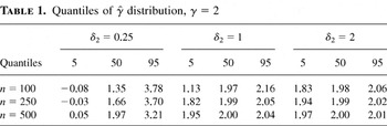
. Table 1 reports the 5%, 50%, and 95% quantiles of the simulation distribution of

, varying δ2 among 0.25, 1, and 2 and n among 100, 250, and 500. Performance improves, as expected, as δ2 and/or n increases. In particular, we observe that for a small threshold effect (δ2 = 0.25), the distribution of

is quite dispersed, whereas a large threshold effect (δ2 = 2) yields a tight sampling distribution, even for a sample size as small as n = 100.
Quantiles of distribution, γ = 2

Second, we assess the performance of our proposed confidence interval

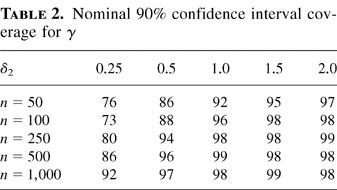
for γ. Table 2 reports simulated coverage probabilities of a nominal 90% interval

, constructed without a correction for heteroskedasticity, varying δ2 among 0.25, 0.5, 1.0, 1.5, and 2.0 and n among 50, 100, 250, 500, and 1,000. We see that for any value of δ2, the coverage probability increases as n increases, becoming fairly conservative for the large sample sizes. Similarly, for fixed n, the coverage probability increases as δ2 increases. These findings do not contradict the distribution theory of Theorem 1, as that result requires that the threshold effect δ2 decreases as n increases, which implies taking a diagonal path in Table 2 roughly from the upper right toward the lower left, where the coverage probabilities indeed fall close to the nominal 90% level. Interestingly, the results in Table 2 are consistent with Theorem 3 of Hansen (2000), which suggests that at least in the leading case of i.i.d. Gaussian errors, the confidence interval

is asymptotically conservative for fixed parameter values as n goes to infinity.
Nominal 90% confidence interval coverage for γ

6.3. Slope Parameters
Theorem 3 shows that the GMM slope estimates

are asymptotically normal and standard errors can be consistently computed from the covariance estimators

. This implies that conventional asymptotic confidence intervals can be constructed based on the normal approximation. We denote this interval as

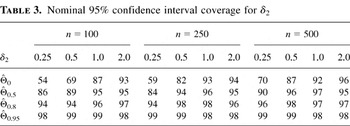
, for reasons given later. In the first row of Table 3 we present the finite sample coverage of nominal 95% confidence intervals for δ2 constructed using this method. We see that if δ2 is large, the interval

has about the correct coverage, but coverage rates are quite poor for small values of δ2. Coverage improves as the sample size n increases, but even for n = 500 coverage is quite poor for small values of δ2.
Nominal 95% confidence interval coverage for δ2

To improve the coverage rates, we can use the Bonferroni-type approach advocated in Hansen (2000). The premise is that the poor coverage rates for

are because it does not take into account uncertainty concerning γ. The solution is to incorporate the confidence interval

for γ developed in Section 4.2.
First, for any fixed value of γ we can calculate the GMM estimators of Section 3.3. Specifically, the sample is split by the indicators 1(qi ≤ γ) and 1(qi > γ), the slope coefficients estimated by GMM on each subsample, and standard errors calculated using the conventional GMM formula. Given these estimates and standard errors, let

denote the constructed C-level confidence region for θ (for this fixed value of γ).
Second, for any 0 ≤ κ < 1, let

denote the confidence interval of Section 4.2 for γ with asymptotic coverage κ.
Third, construct the union of the intervals

, where the union is taken over the values of γ in

,

Theorem 3 shows that

has asymptotic coverage C. Because

it follows that

as n → ∞. Thus the intervals

should be asymptotically conservative.
We report in the four rows of Table 3 the coverage rates of the interval

using κ = 0, 0.5, 0.8, and 0.95. As expected, the coverage rates increase substantially over the

interval. We see that in this example κ = 0.8 provides good coverage in each case, which is the same recommendation as for the regression model investigated in Hansen (2000).
7. CONCLUSION
We have developed consistent estimators for the threshold in a model with endogenous variables and an exogenous threshold variable. The estimator for the threshold is a 2SLS estimator, and the estimator of the slope parameters is a GMM estimator. It may be possible to construct alternative estimators of the parameters based on the GMM principle, and we make no claim to asymptotic efficiency. We specifically focus on the case of an exogenous threshold variable. The case of an endogenous threshold variable would require an alternative estimation approach, and this would be a worthwhile subject for future research.
APPENDIX
Proof of Lemma 1. We need to show that Assumptions 1 and 2 imply equations (15)–(17) for both the reduced form linear model (7) and the reduced form threshold model (8). First, we note the form of

and the rates of convergence of the parameter estimates in these two models. In the linear model (7),

In the threshold model (8), we let ρ0 denote the true value of ρ and write

Then


Equation (A.2) is simple algebra, and equations (A.3)–(A.6) are shown by Chan (1993).
We now sequentially establish (15)–(17).
Proof of (15). First, take the linear model (7).

establishing (15).
Second, take the threshold model (8). Chan (1993) establishes that

Combining this with (A.5), we conclude that

which is (15). █
Proof of (16). By Lemma A.7 of Hansen (2000), there exist constants B and k such that for all η > 0 and ε > 0 there exists a v < ∞ such that for all n

First, take the linear model (7). Using (A.8),

because n1/2|Π −

. Similarly

which is (16).
Second, take the threshold model (8). By (A.8), (A.3)–(A.6), and (A.7), we can pick v, v2, K1, K2, and n so that for all n ≥ n, with probability exceeding 1 − ε,


Using (A.2)

Observe that if v/an ≤ |γ − γ0| ≤ B, then

Hence

Thus with probability exceeding 1 − ε,

We conclude by showing |A1n|K1 ≤ δ/2, which completes the proof of (16). This is simplest when ρ0 ≠ γ0, for then we pick B and n so that

By (A.9) and the triangle inequality,

Expressions (A.13) and (A.14) imply

. Thus for all i

and thus A1n = 0.
For the case ρ0 = γ0, we pick n so that n2α ≥ v/v2. (A.9) implies

and thus for all i

Hence using (A.10), A1n K1 ≤ δ/2 for sufficiently large n. █
Proof of (17). Define

By Lemma A.10 of Hansen (2000),

First, take the linear model (7). Using (A.15) and (A.1),

as desired.
Second, take the threshold model (8). Using (A.2) and (A.15),

where

The proof is completed by showing that A2n = op(1). If γ0 ≠ ρ0, then for large enough n, (|Δi*(v)| + |Δi*(−v)|)|Δ2i(ρ)| = 0 and A2n = 0 with probability arbitrarily close to 1. If γ0 = ρ0, then for large enough n,

and

by (A.7). █ █
Let

. Let G0 be the matrix obtained by stacking the vectors gi′1(qi ≤ γ0).
LEMMA 2. Uniformly in γ ∈ Γ,


Proof of Lemma 2. To show (A.16), because

, using (15) and Lemma 1 of Hansen (1996),

uniformly in γ ∈ Γ. Equation (A.17) follows similarly. To show (A.18), using Lemma A.4 of Hansen (2000) and (15),

LEMMA 3.

.
Proof of Lemma 3. It will be convenient to write (5) in the format

Define the matrices

by stacking

. This equation can be written in matrix format as

where we use δn = cn−α.
Let

where

. Because

, it can be shown that Pγ* = Pγ + P⊥.
Because

is in the span of

, then

Thus using (A.19),

Hence

Because the first term in the last expression does not depend on γ, and

minimizes Sn(γ), we see that

maximizes

From Lemma 2, we see that uniformly in γ ∈ [γ0,γ],

When γ > γ0 then P⊥ G0 = 0, so Pγ*G0 = Pγ G0 and

uniformly on γ ∈ [γ0,γ], which is uniquely maximized at γ0 as shown in the proof of Lemma A.5 of Hansen (2000). Symmetrically, on γ ∈ [γ,γ0], Sn*(γ) converges uniformly to a limit function uniquely maximized at γ0. Because

maximizes Sn*(γ), it follows that

. █
LEMMA 4.

.
Proof of Lemma 4. Let the constants B, d, k be defined as B > 0, 0 < d < ∞, 0 < k < ∞. Let M = sup|γ−γ0|≤B|M(γ)−1| and D = sup|γ−γ0|≤B|D1(γ) f (γ)|. Fix ε > 0. Pick κ and reduce B if necessary so that


where M* = M + M2κ and M0 = M(γ0). To simplify some inequalities, assume without loss of generality that κ ≤ k.
Define

Define the joint event


By Lemma A.7 of Hansen (2000) and (16), there exist sufficiently large v = v(ε) < ∞ and n = n(ε) < ∞ so that for all n ≥ n, equations (A.24)–(A.27) hold jointly with probability exceeding 1 − ε/2. By Lemmas 2 and 3, equations (A.28)–(A.32) hold jointly with probability exceeding 1 − ε/2 (increasing n if necessary). Thus (A.24)–(A.32) hold jointly with probability exceeding 1 − ε.
We show subsequently that (A.24)–(A.32) imply


Using (A.20) and applying (A.33)–(A.35) we can calculate that for v/an ≤ |γ − γ0| ≤ B, (A.24)–(A.32) imply

Because

, this establishes that (A.24)–(A.32) imply

. As discussed previously, (A.24)–(A.32) hold jointly with probability exceeding 1 − ε for all n ≥ n. Thus

for n ≥ n as required.
The proof is completed by showing that (A.24)–(A.32) imply (A.33)–(A.35).
For simplicity, we restrict attention to the region [γ0 + v/an ≤ γ ≤ γ0 + B], as the analysis for the case [γ0 − v/an ≥ γ ≥ γ0 − B] is similar. This restriction implies

so (P0* − Pγ*)G0 = (P0 − Pγ)G0.
We start with some useful bounds. Equation (A.30) implies

Equations (A.29), (A.31), (A.36), and a Taylor's expansion imply

Expressions (A.31), (A.32), and (A.36) imply

and

Next, observe that

Equations (A.24)–(A.27) imply


and

We can now show (A.33). We calculate that

Hence, using (A.37), (A.38), (A.41), and (A.42),

the last inequality being (A.21). This is (A.33).
Next, we show (A.34). We calculate that

Hence, using (A.38), (A.39), (A.41) and (A.43),

the last inequality being (A.22). This is (A.34).
Finally, we show (A.35). Observe that

We examine the first term of (A.46). We calculate that

Hence using (A.39), (A.41), and (A.43),

the last inequality being (A.23). A similar argument applies to the second term of (A.46). Together, we find

This is (A.35) and completes the proof. █
LEMMA 5. On [−v,v],

where μ = c′D1 cf and λ = c′D2 cf.
Proof of Lemma 5. Reparameterize all functions of γ instead as functions of ν. For example, Zν = Zγ0+ν/an, Pν = Pγ0+ν/an, Δi(ν) = Δi(γ0 + ν/an). We show subsequently that uniformly on ν ∈ [−v,v],


Using (A.20) and (A.48)–(A.50), we find

as stated. The proof is completed by demonstrating (A.48)–(A.50).
First, observe that using the decomposition (A.40), Lemma A.10 of Hansen (2000), and (17), we have

so

Second, by Lemma 2

Then, by (A.44), (A.51), (A.52), Lemma 2, (A.40), (17), and Lemma A.10 of Hansen (2000),

This is (A.48).
By Lemma 2 and (A.52), uniformly in ν ∈ [−v,v],

By (17)

a vector Brownian motion with covariance matrix D2 f, where the final convergence uses Lemma A.11 of Hansen (2000). Thus by (A.45), (A.51), (A.52), (A.53), and (A.54),

This yields (A.49).
Finally, by (A.47), (A.51), (A.53), and (A.54)

uniformly in ν ∈ [−v,v]. A similar argument applies to

. Combined with (A.46) this establishes (A.50) and completes the proof. █
Proof of Theorem 1. By Lemma 4,

and by Lemma 5, Qn(ν) ⇒ −μ|ν| + 2λ1/2W(ν), where the limit functional is continuous with a unique maximum almost surely. Appealing to Theorem 2.7 of Kim and Pollard (1990), (18) and (19) follow by the argument in the proofs of Theorem 1 and 2 of Hansen (2000). █
The 2SLS and GMM estimators of θ1 and θ2 introduced in Section 3 are special cases of the class of estimators


where

are sequences of weight matrices.
LEMMA 6. If

then

where


Proof of Lemma 6. We provide the details of the proof for θ1. Let Zv, Z⊥, ΔZv, Xv denote the matrices obtained by stacking, respectively,

By Lemma 1 of Hansen (1996), Lemma A.4 of Hansen (2000), and Lemma A.10 of Hansen (2000), uniformly on ν ∈ [−v,v],


Let

A little rewriting of the model shows that

Uniformly on ν ∈ [−v,v] , by (A.59)–(A.61),

Because

, it follows that

as stated. █
Proof of Theorem 2. The 2SLS estimators

fall in the class (A.55) and (A.56) with

By Lemma 1 of Hansen (1996) and the consistency of

. Thus

are asymptotically normal, with covariance matrices given by the formula (A.57) and (A.58) with Q1 and Q2 replacing W1 and W2, yielding the stated result. █
Proof of Theorem 3. Let

It will be enough to show that

uniformly in γ ∈ Γ, for then by the consistency of

, and the theorem follows by Lemma 6. Hence we show (A.62).
Set

. Algebraic manipulation shows that

Hence

It is straightforward to show that the terms on the right-hand side converge in probability to zero, uniformly in γ. For example, the first term is bounded by

because the data have bounded fourth moments and

. Hence,

uniformly in γ, by Lemma 1 of Hansen (1996), which is (A.62). This completes the proof. █
Proof of Theorem 4. Under the null of θ1 = θ2,

Then by Lemma 1 of Hansen (1996) and Assumption 1.3, uniformly in γ

Via Lemma A.4 of Hansen (2000)

Use (A.63) and (A.64) with (A.62) to have

In the same manner we derive

A similar argument applies to the covariance matrices. Combining these results completes the proof. █
References
REFERENCES
Andrews, D.W.K. &
V. Ploberger
(1994)
Optimal tests when a nuisance parameter is present only under the
alternative.
Econometrica
62,
1383–1414.Google Scholar
Bai, J.
(1997)
Estimation of a changepoint in multiple regression models.
Review of Economics and Statistics
79,
551–563.Google Scholar
Barnett, S.A. &
P. Sakellaris
(1998)
Nonlinear response of firm investment to q: Testing a
model of convex and non-convex adjustment costs.
Journal of Monetary Economics
42,
261–288.Google Scholar
Bhattacharya, P.K. &
P.J. Brockwell
(1976)
The minimum of an additive process with applications to signal
estimation and storage theory.
Zeitschrift für Wahrscheinlichskeitstheorie und Verwandte
Gebiete
37,
51–75.Google Scholar
Caner, M.
(2002)
A note on LAD estimation of a threshold model.
Econometric Theory
18,
800–814.Google Scholar
Chamberlain, G.
(1987)
Asymptotic efficiency in estimation with conditional Monet
restrictions.
Journal of Econometrics
34,
305–334.Google Scholar
Chan, K.S.
(1993)
Consistency and limiting distribution of the least squares
estimator of a threshold autoregressive model.
Annals of Statistics
21,
520–533.Google Scholar
Davies, R.B.
(1977)
Hypothesis testing when a nuisance parameter is present only under
the alternative.
Biometrika
64,
247–254.Google Scholar
Erickson, T. &
T.M. Whited
(2000)
Measurement error and the relationship between investment and
q.
Journal of Political Economy
108,
1027–1057.Google Scholar
Fazzari, S.M.,
R.G. Hubbard, &
B.C. Petersen
(1988)
Financing constraints and corporate investment.
Brookings Papers on Economic Activity
1,
141–195.Google Scholar
Hansen, B.E.
(1996)
Inference when a nuisance parameter is not identified under the
null hypothesis.
Econometrica
64,
413–430.Google Scholar
Hansen, B.E.
(1999)
Threshold effects in non-dynamic panels: Estimation, testing, and
inference.
Journal of Econometrics
93,
345–368.Google Scholar
Hansen, B.E.
(2000)
Sample splitting and threshold estimation.
Econometrica
68,
575–603.Google Scholar
Hu, X. &
F. Schiantarelli
(1998)
Investment and capital market imperfections: A switching regression
approach using U.S. firm panel data.
Review of Economics and Statistics
80,
466–479.Google Scholar
Picard, D.
(1985)
Testing and estimating change-points in time series.
Advances in Applied Probability
17,
841–867.Google Scholar
Quantiles of distribution, γ = 2
Nominal 90% confidence interval coverage for γ
Nominal 95% confidence interval coverage for δ2
 You have
Access
- 595
- Cited by