2. THE HSR POLICY IS OPTIMAL

Recall the setup presented in (1) and (2). To begin with, assume that the arrival process is deterministic, with arrivals at time points s_j,j ≥ 1, such that

Set s₀ = 0. We will prove that the HSR policy implies (1) by induction, using the following idea: Suppose we have been able to construct

on [0,s_j] in such a way that (1) holds for t ∈ [0,s_j] and the states of

at t = s_j are feasible, in a sense to be made precise later, then we will be able to extend that to the interval [0,s_j+1] , for j = 1,2,…

It is due time for the details. Because the service times are exponentially distributed, the states of

are completely described by the number of customers and the configurations of busy stations. Let

and for b = (b₁,…,b_k) ∈ B,

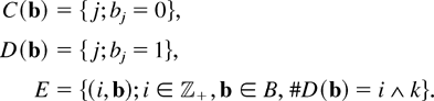
That a system is in state (i,b) ∈ E will mean that there are i customers in it, with the configuration of busy stations given by b; b_j = 1 indicates that station j is busy.

For the partial ordering on E that will be defined now, let D(b) ≠ [empty ] to start. We define [prcue ] on E as follows: For i ≥ 1,

exactly when the following hold:

To complete the definition, let (0,(0,…,0)) [prcue ] (i′,b′) for all (i′,b′) ∈ E.

The meaning of (6(ii)) is that we can match each busy station in

with one busy station in

with a smaller or equal service rate.

We will use X_t = (Y_t,B_t), t ≥ 0, to denote queuing process when the HSR policy is used and use X_t′ = (Y_t′,B_t′), t ≥ 0, to denote the competing process with some other routing policy; the meanings of B_t and B_t′, t ≥ 0, are the obvious ones. We will produce a coupling such that X_t [prcue ] X_t′ for all t ≥ 0, under the assumption that the initial distributions are the same.

We follow the convention about right-continuity of paths of the type of processes we are dealing with here. That means that we will produce (X_t,X_t′), t ≥ 0, as a time-homogeneous jump Markov process on each of the intervals [s_j,s_j+1), j = 0,1,…, and then pay special attention to the jump at s_j+1. We are now able to be precise about what the proof idea requires:

We used the word “feasible” in the presentation of the proof idea; now (7(ii)) makes that precise. We will apply (7) to the intervals [s_j,s_j+1], j = 0,1,…, successively, with X₀ = X₀′ for the application to the interval [0,s₁] . That yields

if X₀ = X₀′, which is actually stronger than (1).

For (7(i)), recall the properties of the mappings φ(b,b′,·) in (6(ii)) and that the stations have intensities δ₁,…,δ_k satisfying δ₁ ≥ ··· ≥ δ_k.

Let e_j = (0,…,1,…0) be the jth unit vector. For convenience, we will occasionally abbreviate φ(b,b′,j) to j′.

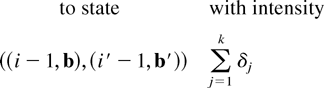
We will produce (X_t,X_t′), t ≥ 0, in terms of transition intensities. Fix two elements in E such that (i,b) [prcue ] (i′,b′), to be thought of as states of X₀ and X₀′, respectively. We sort out the presentation of the intensities into three cases.

Case 1: i > k. From ((i,b),(i′,b′)), we make a jump

Case 2: i ≤ k,i′ ≤ k. From ((i,b),(i′,b′)), we make jumps

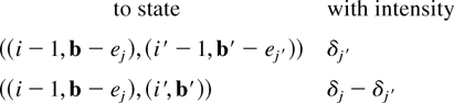
for j ∈ D(b) and

for j ∈ D(b′)[setmn ]φ(D(b)) if that set is not equal to [empty ], which implies i < i′.

Case 3: i ≤ k,i′ > k. From ((i,b),(i′,b′)), we make jumps

for j ∈ D(b) and

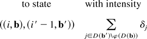
Clearly, all possible jumps go to states ∈ E × E with the inequality [prcue ] preserved.

We turn to (7(ii)). It is obvious how the HSR policy works. However, we have not defined what is meant by a routing policy in general: It is a rule that decides about an arrival customer, given the state of the system at the arrival. If there is at most one station idle, the rule is the trivial one; there is no choice. The rule could mean a randomization over idle stations; we omit the formalism involving a Markov kernel on E × E and think of

using a policy deviating from the HSR policy.

Now, let (i,b) and (i′,b′) be the states of X_T− and X_T−′, respectively, and let (i + 1,b*) and (i′ + 1,b*′) denote the states at X_T and X_T′. We have to find a function φ(b*,b*′,·) satisfying (6(ii)).

If i′ ≥ k, the arriving customer to

at time T finds all stations busy. That means that we may let

Therefore, suppose that i′ < k. Clearly, due to the HSR policy,

where

We observe that {1,…,m − 1} ⊆ D(b).

Suppose that the policy for

routes the customer arriving at time T to station [ell ]. To start, suppose that [ell ] < m. Let

Since φ(b,b′,·) is strictly increasing on D(b) and {1,…,m − 1} ⊆ D(b), L is either empty or a set {1,…,r} ⊆ {1,…,m − 1} for some r ≥ 1.

If L = [empty ], let

If L ≠ [empty ], let

A similar proof applies to the case [ell ] ≥ m; let r be the integer ∈ {0,…,k − 1} such that L = {1,…,r} ∩ D(b) (= [empty ] if r = 0) and note that special attention has to be paid to the case r ≥ m.

That completes the proof of (8), for an arrival process satisfying (4). However, the condition in (4) excluding multiple arrivals was made to avoid some trite arguments; with multiple arrivals, we extend (7) to cover the case: T = 0 and (7(i)) dropped. No obstacles appear.

For a random point process ξ of arrivals, let S = (S_i)₁^∞ be its points of occurrence in increasing order. If ξ is independent of the service times involved, then (8) is seen to hold for the random arrival case, after a conditioning on S.

That completes the proof of the optimality of the HSR policy; we refrain from a statement in terms of a theorem.

Remarks:

4. For this remark, suppose that the HSR policy is used for both

and that the arrivals appear according to a time-homogeneous Poisson process (which renders X_t,t ≥ 0, a Markov process). It is clear from the proof of (8) that if

is idle at time 0, then X_t [prcue ] X_t′ for all t ≥ 0, regardless of the initial configuration of

. That is the condition of Lindvall [2, Sect. IV.3, Thm. (9.3)] and we can conclude from that theorem that X_t is stochastically increasing in t if

is idle at time 0; the same monotonicity for Y_t follows.

3. USE FEW BUT QUICK STATIONS

In Lindvall [3, Sect.6], it was proved that if we compare two M/M/· systems, with k and k′ stations and service rates δ and δ′, respectively, where k < k′ and kδ = k′δ′, then (1) holds if Y₀ ≤ Y₀′, for a certain natural and simple coupling. That speaks in favor of the design principle: Use few but quick stations.

We will now generalize that result to the case where the service rates δ₁,…,δ_k and δ₁′,…,δ_k′′ of the stations in

, respectively, satisfy

and the arrival process is arbitrary but independent of the service times, as in Section 2. It is assumed that the HSR policy is used for both

, but it suffices that

uses that policy. We will be as brief as possible, concentrating on the necessary modification of the setup in Section 2 and a new coupling problem that has to be solved.

Some new notation is needed. Let

we let C(b′) and D(b′) have their obvious meanings for b′ ∈ B′. For the matching in (6(ii)), the mapping φ(b,b′,·) now has {1,…,k′} as its range. That means that (6(i)) and (6(ii)) no longer define a partial ordering on E, but rather a relation on E × E′; that is, however, sufficient for our purposes. We use

to denote that relation.

We will produce (X_t,X_t′),t ≥ 0, such that

when

. Clearly, that implies (1).

We will pay no attention to the analog of (7(ii)), since the proof of that is virtually the same as for the routing problem. For the analog of (7(i)), let (i,b) ∈ E and (i′,b′) ∈ E′ be such that

; we will produce couplings such that “inequality” is preserved when services are finished. Note that i ≤ i′.

Case 1°: i ≤ k. Use the obvious variants of Cases 2 and 3 in Section 2.

For the case i > k, we need couplings that are more subtle than those above. To that end, let

Further, let

Here, [ell ](I) denotes the length of an interval I.

Case 2°: i > k,i′ = k′. Let φ(b,b′,j) = j for j = 1,…,k. From ((i,b),(i′,b′)), we make jumps

for j = 1,…,k,

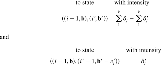
for j = k + 1,…,k′.

To understand the last intensity, consider γ_mn as the intensity for service finished both at station m in

and station n in

. We have

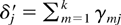
due to the condition

. Because there is a customer waiting in

, it does not become visible which station in

finishes service at the same time as station j in

.

We used e_j′ to denote the jth k′-dimensional unit vector.

Case 3°: i > k,i′ > k′. This case is easy, after understanding Case 2°.

Case 4°: i > k,i′ < k′. Let n₁′,…,n_m′ be the elements of D(b′) enumerated in increasing order and let

Now use an obvious variant of Case 2°.

For Cases 1°–4°, we find that the relation

is preserved after jumps; hence (11) is proved.