
 Gn
 Gn





1. Introduction
A temporal graph (see Figure 1) is an edge-labeled graph
 $\mathcal{G}= (G, \sigma)$
where the underlying graph
 $G = (V(G),E(G))$
is a finite simple graph and
 $\sigma\colon E(G)\rightarrow \{1,\dots, |E(G)|\}$
is an ordering of the edges. In this paper we consider random temporal graphs in which
 $\sigma(E(G))$
is a uniform random permutation. Equivalently, we can generate a random temporal graph using independent, uniform, labels: each edge
 $e\in E(G)$
is assigned a label
 $\tau_e\sim \mathrm{Unif}[0,1]$
. For
 $e\in E(G)$
we say that
 $\tau_e$
is the time-stamp of e, and for
 $f\in E(G)\setminus \{e\}$
, we say that e precedes f if
 $\tau_e \le \tau_f$
. We use this construction in the sequel, and denote the resulting graph as
 $\mathcal{G}= (G, (\tau_e)_{e\in E(G)})$
.
A temporal random geometric graph on
 $[0,1]^2$
where edges that are coloured darker arrive later (left), and its longest monotone increasing path (right).

The study of such graphs is largely motivated by the modeling of dynamic networks [Reference Tang, Leontiadis, Scellato, Nicosia, Mascolo, Musolesi and Latora14]. A temporal graph represents a network where interactions occur at particular times. In temporal networks we can study whether it is possible to transmit information, or an infectious disease, from one individual to another, as a chain of transmissions can only occur along interactions that are increasing in time.
Let
 $\mathcal{G}= (G, (\tau_e)_{e\in E(G)})$
be a temporal graph. For vertices
 $u,v\in V(G)$
we say that there is a temporal path from u to v, denoted
 , if there exists a path from u to v comprised of non-decreasing edge time-stamps. Further, we let
 denote the length of the shortest temporal path from u to v, that is, the minimal number of edges on any monotone increasing path from u to v. It is readily seen that the existence of a temporal path
does not imply the existence of a temporal path
 , and furthermore the existence of temporal paths
and
 does not imply the existence of a temporal path
 . Following the terminology of [Reference Becker, Casteigts, Crescenzi, Kodric, Renken, Raskin and Zamaraev3], we say that a vertex
 $u\in\mathcal{G}$
is a temporal source if there exist temporal paths
 for all
 $v\in\mathcal{G}$
. Moreover, we call
 $\mathcal{G}$
temporally connected if every vertex of
 $\mathcal{G}$
is a temporal source.
The temporal random graph model can be seen as a random version of a well-known combinatorial problem posed in [Reference Chvátal and Komlós8], which asks for the minimal value of the length of the longest monotone path, when considering the edge orderings of the complete graph on n vertices, henceforth denoted by
 $K_n$
. This problem is well studied, with lower and upper bounds remaining far apart until recent years; see, e.g., [Reference Bucić, Kwan, Pokrovskiy, Sudakov, Tran and Wagner5, Reference Calderbank, Chung and Sturtevant6, Reference Graham and Kleitman9]. The average case with base graph
 $G = K_n$
was first considered in [Reference Lavrov and Loh11] and [Reference Martinsson12] later proved that, with high probability, there exists a monotone path of length
 $n-1$
. When G is an Erdős–Rényi random graph, the resulting temporal graph is called the random simple temporal graph, first studied in [Reference Angel, Ferber, Sudakov and Tassion1].
Temporal connectivity of random simple temporal graphs was studied in detail in [Reference Becker, Casteigts, Crescenzi, Kodric, Renken, Raskin and Zamaraev3, Reference Casteigts, Raskin, Renken and Zamaraev7]. In particular, it is shown in [Reference Casteigts, Raskin, Renken and Zamaraev7] that the threshold for temporal connectivity of random simple temporal graphs is
 ${\sim} 3\log n/n$
, which is just a factor of three larger than the connectivity threshold of the underlying Erdős–Rényi random graph. More recent works have studied the shortest and longest increasing paths between typical vertices [Reference Broutin, Kamčev and Lugosi4] and the size of the largest temporal clique [Reference Atamanchuk, Devroye and Lugosi2].
In this paper, we initiate the study of temporal random geometric graphs. In this model the vertices of the underlying graph
 $G_n$
correspond to randomly drawn points in a Euclidean space. Such graphs may be better suited for modeling epidemiological processes than random simple temporal graphs, as the geometry allows for spatial closeness (or closeness encoding similarity) of individuals to affect interaction probabilities. Our main results establish thresholds for temporal connectivity in certain temporal random geometric graphs.
For
 $d\ge 2$
, let
 $\|\cdot \|$
denote the Euclidean distance on the d-dimensional unit torus,
 $[0,1]^d$
. Let
 $K\colon[0,\infty) \rightarrow [0,1]$
be a non-increasing function. Further, let
 $n \in \mathbb{N}$
and
 $r_n > 0$
. A soft random geometric graph
 $G_n = (\mathcal{X}_n, K, r_n)$
in dimension d is a graph on n uniform random points
 $\mathcal{X}_n$
in the unit torus
 $[0,1]^d$
such that, for every pair of vertices
 $u,v\in \mathcal{X}_n$
, an edge exists with probability
 $\mathbb{P}\{ {uv} \in E(G_n)\mid \mathcal{X}_n\} = K({\|u-v\|}/{r_n})$
. The edges are conditionally independent given
 $\mathcal{X}_n$
. When
 $K(x) := \mathbf{1}_{[x \leq 1]}$
,
 $G_n$
is called a hard random geometric graph. A temporal random geometric graph with n vertices is a temporal graph
 $\mathcal{G}_n = (G_n, (\tau_e)_{e\in E(G_n)})$
where
 $G_n = (\mathcal{X}_n, K, r_n)$
is a soft random geometric graph on n vertices. Our main result shows that under regularity conditions on K, with high probability, the graph becomes temporally connected when the radius
 $r_n$
exceeds a constant multiple of
 $n^{-1/(d+1)}$
, while the graph is temporally disconnected if
 $r_n$
is smaller than another constant times
 $n^{-1/(d+1)}$
.
Theorem 1.1. Let
 $\mathcal{G}_n = (G_n, (\tau_e)_{e \in E(G_n)})$
be a temporal random geometric graph with
 $G_n = (\mathcal{X}_n, K,r_n)$
satisfying the following:
-
[A1] There exists
 $\alpha > 0$
such that K(x)
$\geq \alpha$
for all
$x \leq 1$
.
-
[A2] For
$x > 1 \text{, }K(x) \leq \beta x^{-d}{\mathrm{e}}^{-{2}(x+1)\log(x+1)}$
for some
$\beta > 0$
.




Then there exist constants
 $c_d, C_d> 0$
such that
-
(i) if
$r_n \leq c_d n^{-1/(d+1)}$
for all n sufficiently large, then
$\mathcal{G}_n$
is asymptotically almost surely (a.a.s.) temporally disconnected; -
(ii) if
$r_n \geq C_d n^{-1/(d+1)}$
for all n sufficiently large, then
$\mathcal{G}_n$
is a.a.s. temporally connected.



Observe that, by the monotonicity of temporal connectivity, Theorem 1.1 implies that (i) holds under just assumption [A2] and (ii) holds under just assumption [A1].
Note that the choice of
 $K(x) = \mathbf{1}_{[x \leq 1]}$
satisfies the regularity conditions [A1] and [A2], and therefore as a corollary of Theorem 1.1 we obtain a threshold for asymptotically almost sure temporal connectivity of temporal hard random geometric graphs. Assumptions [A1] and [A2] ensure that there are sufficiently many vertices at graph distance
 $O(r_n)$
to any vertex, and that there are not too many long edges in the soft random geometric graph.
Observe that the order of magnitude
 $n^{-1/(d+1)}$
of the critical radius is significantly larger than that of the critical radius for the connectivity of the underlying random geometric graph. Indeed, as is well known from the theory of random geometric graphs, random geometric graphs become connected when the average degree of the graph is of order
 $\log n$
[Reference Penrose13]. On the other hand, our results show that temporal connectivity only occurs when the average degree becomes of order
 $n^{1/(d+1)}$
. This is in stark contrast with Erdős–Rényi random graphs in which temporal connectivity and simple connectivity both occur when the average degree is of the order of
 $\log n$
. The regime
 $r_n\approx n^{-1/(d+1)}$
is somewhat unusual, as we are not aware of any other natural phase transition happening in random geometric graphs in this range.
Theorem 1.1 establishes the order of magnitude of the temporal connectivity threshold. It is natural to conjecture that, similarly to the case of Erdős–Rényi graphs, there is a sharp threshold for temporal connectivity, that is, there exists a constant
 $\kappa_d$
(depending on the kernel K) such that, for all
 $\varepsilon >0$
, if
 $r_n \le (\kappa_d-\varepsilon)n^{-1/(d+1)}$
then
 $\mathcal{G}_n$
is a.a.s. temporally disconnected, while for
 $r_n \ge (\kappa_d+\varepsilon)n^{-1/(d+1)}$
 $\mathcal{G}_n$
is a.a.s. temporally connected. Our techniques are not sufficiently strong to establish such results and we leave the problem of the existence of a sharp threshold and the value of
 $\kappa_d$
for challenging future research.
Various definitions of temporal connectivity were introduced in [Reference Becker, Casteigts, Crescenzi, Kodric, Renken, Raskin and Zamaraev3]. In particular, for the case of random simple temporal graphs, they establish sharp thresholds for the probability of the existence of a temporal path between two typical vertices and for the probability of a typical vertex being a temporal source. It is an interesting question to study these probabilities, along with the probability of temporal connectivity. As is apparent from our proofs, the critical radius for all these quantities is of the same order of magnitude, but we have no further information about their relationship.
The random geometric graph considered in this paper is defined on the unit torus. One can similarly set up the problem by considering the hypercube
 $[0,1]^d$
with the usual Euclidean distance. The setups are quite similar, and our choice makes it possible to avoid some technicalities arising from edge effects. We believe that is is quite straightforward to modify the proofs to extend the result of Theorem 1.1 to the Euclidean setting.
We can also consider the problem when
 $d=1$
. This case is considerably less complex, and a straightforward simplification of the proof of Theorem 1.1 shows that the theorem also holds in the one-dimensional case (i.e. the threshold for temporal connectivity is of the order of
 $n^{-1/2}$
).
In Section 2 we prove the upper bound of Theorem 1.1, i.e. we determine a threshold for when
 $\mathcal{G}_n$
is a.a.s. temporally disconnected. In Section 3 we prove the lower bound of Theorem 1.1 by mapping the construction of a temporal path to a directed percolation model.
2. Upper bound:
$\mathcal{G}_{\boldsymbol{{n}}}$
temporally disconnected

Let
 $\mathcal{G}_n = (G_n, (\tau_e)_{e \in E(G_n)})$
be a temporal random geometric graph with
 $G_n = (\mathcal{X}_n, K, r_n)$
satisfying assumptions [A1] and [A2]. In this section, we prove that there exists
 $c>0$
such that if
 $r_n\leq cn^{-1/(d+1)}$
for all n sufficiently large, then a.a.s.
 $\mathcal{G}_n$
has a vertex that is not a temporal source (and in particular
 $\mathcal{G}_n$
is not temporally connected). In fact, the following proposition shows that not only does there a.a.s. exist a vertex that is not a temporal source, but that in fact a.a.s. no vertex is a temporal source in this regime.
Proposition 2.1. Suppose that
 $\mathcal{G}_n = (G_n, (\tau_e)_{e\in E(G_n)})$
is a temporal random geometric graph with
 $G_n = (\mathcal{X}_n, K, r_n)$
satisfying assumptions [A1] and [A2]. Then there exists
 $c > 0$
such that if
 $r_n \le cn^{-1/(d+1)}$
for all n sufficiently large, then

Proof. Assume
 $r_n = c n^{-1/(d+1)}$
for some
 $c > 0$
. We show that (2.1) holds, and the proposition then follows by the monotonicity of temporal connectivity.
The event of having a temporal source is contained in the union of the following three events: all points
 $\mathcal{X}_n$
are contained in a ball of radius at most
 $\sqrt{d}(1-r_n)/2$
around some point in
 $\mathcal{X}_n$
; there exists a long temporal path of length at least
 $1/3r_n$
; or there exists a short temporal path between two points at distance at least
 $\sqrt{d}(1-r_n)/2$
. More precisely,

Thus, it suffices to show that each of the terms on the right-hand side of (2.2) is o(1).
Note that by applying a union bound to the first term of (2.2), we may consider each fixed vertex
 $u\in \mathcal{X}_n$
to be the point
 $\big(\frac12, \frac12\big)$
without loss of generality. Therefore, the first term is at most
 \begin{align} n\cdot{\mathbb P}\bigg\{\text{for all } v \in \mathcal{X}_n,\, \big\|\big(\tfrac{1}{2}, \tfrac{1}{2}\big) - v\big\| < \frac{\sqrt{d}}{2}(1-r_n)\bigg\} & \le n\cdot{\mathbb P}\bigg\{\bigg[1-\frac{r_n}{2},1\bigg]^d\cap\mathcal{X}_n=\emptyset\bigg\} \nonumber \\ & = n\bigg(1 - \bigg(\frac{r_n}{2}\bigg)^d\bigg)^{n} \nonumber \\ & \le \exp\bigg[\log n - n\bigg(\frac{r_n}{2}\bigg)^d\bigg] \nonumber \\ & = o(1), \end{align}
where the final equality holds as
 $r_n = cn^{-1/(d+1)} \gg (\log n/n)^{1/d}$
for any
 $c > 0$
.
To bound the second term, we apply the first-moment method. To this end, without loss of generality, assume that
 $1/{3}r_n\in \mathbb{N}$
, let
 $k = 1/{3}r_n$
, and let
 $N_n^{(k)}$
denote the number of temporal paths in
 $\mathcal{G}_n$
with at least
 $k-1$
edges. By choosing k ordered vertices and ensuring that the edges between them exist and have monotone increasing labels, it follows that
 \begin{equation*} {\mathbb E}\big[N_n^{(k)}\big] \leq \binom{n}{k}k!\frac{1}{{(k-1)!}} \bigg({c_d'}r_n^d + \int_{[0,1]^d \setminus \mathcal{B}(0,r_{{n}})}K(\|y\|/r_n)\,{\mathrm{d}} y\bigg)^{k-1}, \end{equation*}
where
 $c_d' > 0$
is the volume of the unit ball in the d-dimensional torus. By our conditions on K, the integral in the above inequality is at most a constant multiple,
 $\gamma_d > 0$
, of
 $r_n^d$
. We note that both
 $c_d'$
and
 $\gamma_d$
may be uniformly bounded over all
 $d\ge 2$
. Therefore, together with the bound
 $\binom{n}{k}\le ({{\mathrm{e}} n}/{k})^k$
, it follows that there exists
 ${\lambda}> 0$
such that
 \begin{align} {\mathbb E}\big[N_n^{(k)}\big] & \leq {\lambda}^{k-1}\bigg(\frac{{\mathrm{e}} n}{k}\bigg)^k k r_n^{d(k-1)} \nonumber \\ & = {\lambda}^{k-1}\exp[k\log n + k - (k-1)\log k + d(k-1)\log(r_n)] \nonumber \\ & \le \lambda^{k-1}\exp[k\log n + k - (k-1)\log k - d(k-1)\log k] \nonumber \\ & \le {\lambda}^{k-1}\exp\bigg[k\log n + k\bigg(1-(d+1)\frac{k-1}{k}\log k\bigg)\bigg]. \end{align}
Given our choice of
 $r_n = cn^{-1/(d+1)}$
for some
 $c > 0$
, for n sufficiently large we have that
 $\log k = \log (1/3r_n) \ge \log(1/3c) + \log(n)/(d+1)$
and so (2.4) is at most
 \begin{equation} {\lambda}^{k-1}\exp\bigg[\log n + \bigg(1-(d+1)\log\bigg(\frac{1}{3c}\bigg)\bigg)k + (d+1)\log\bigg(\frac{1}{3c}\bigg)\bigg], \end{equation}
which is o(1) if
 $c > 0$
. Since any temporal path of length at least
 $k = 1/3r_n$
must include a sub-path of length
 $k-1$
, combining (2.5) with the first-moment method yields

From (2.3) and (2.6), we have that the first two terms in (2.2) are o(1). Thus, it remains to prove that connectivity via short paths is unlikely for vertices which are geometrically far apart, i.e. to show that

First, note that we can work under the event that for every edge
 $uv \in E(G_n)$
,
 $\|{u-v}\| \leq r_n \log n$
, since the probability that there exists an edge of length greater than
 $r_n \log n $
is, by a union bound, at most
 \begin{align*} n^2{\mathbb P}\{uv \in E(G_n) \mid u,v\in\mathcal{X}_n\} \leq n^2 K(\log n) = O(n^2{\mathrm{e}}^{-\log n \log\log n}) = o(1) \end{align*}
for u, v satisfying
 $\|u-v\| > r_n \log n$
.
For sufficiently large n, we have
 $\sqrt{d} (1-r_n) /2 \geq \frac13$
so we can bound the left-hand side of (2.7) from above by the probability that there exists a temporal path
with
 $M\in((3r_n\log n)^{-1},(3r_n)^{-1})\cap\mathbb{N}$
edges, such that the sum of its edge lengths is at least
 $\frac13$
. For
 $M\in((3r_n\log n)^{-1},(3r_n)^{-1})\cap\mathbb{N}$
we denote this event by
 $A^M_n$
. Further, for
 $L \in \mathbb{N}$
and
 $M \in ((3r_n\log n)^{-1},(3r_n)^{-1})\cap\mathbb{N}$
, let
 $N_{M,L}$
denote the number of temporal paths
with M edges with respective lengths
 $d_1,\dots,d_M$
such that
 $\sum_{i=1}^M\lceil d_i r_n^{-1}\rceil = L$
. Then, by a union bound,
 \begin{equation} {\mathbb P}\Bigg\{\bigcup_{M\in({1}/{3r_n\log n},{1}/{3r_n})\cap\mathbb{N}}A_n^M\Bigg\} \le \sum_{M=\lceil {1}/{3r_n\log n}\rceil}^{\lfloor {1}/{3r_n}\rfloor}\sum_{L \ge r_n^{-1}/3}{\mathbb E}[N_{M,L}]. \end{equation}
To prove (2.7), it therefore suffices to show that the right-hand side of (2.8) is o(1). To this end, consider a path in
 $G_n$
with M edges of respective lengths
 $d_1,\dots, d_M$
such that
 $\sum_{i=1}^M d_i \ge \frac13$
. These edge lengths correspond to a vector
 $(\ell_i)_{i\in [M]}$
where, for all
 $i\in [M]$
,
 $\ell_i := \lceil d_i r_n^{-1}\rceil\in\mathbb{N}$
. With
 $L = \sum_{i=1}^M \ell _i$
, we have
 $L \ge (3r_n)^{-1}$
.
For a given L, the number of such vectors is bounded from above by
 \begin{align*}\binom{L-1}{M-1} \leq \bigg(\frac{{\mathrm{e}} L}{M}\bigg)^M = {\mathrm{e}}^{M\log(L/M) + M}.\end{align*}
Recall that the volume of the unit ball in
 $\mathbb{R}^d$
,
 $c_d'$
, is uniformly bounded above by
 $\lambda$
. Fixing
 $(\ell_i)_{i\in M}$
and a set of distinct vertices
 $(v_i)_{i \in [M+1]}$
, the probability that the temporal path
 exists in
 $G_n$
, i.e. that
 $v_i v_{i+1} \in E(G_n)$
for each
 $i \in [M]$
where the edge length between
 $v_i$
and
 $v_{i+1}$
is in
 $[(\ell_i -1)r_n, \ell_i r_n]$
, can be bounded from above by
 \begin{align*} \prod_{i=1}^M\lambda\int_{(\ell_i-1) r_n}^{\ell_ir_n}K(\xi/r_n)\xi^{d-1}\,{\mathrm{d}}\xi & = \left(\lambda r_n^d\right)^M\prod_{i=1}^M\bigg(\int_{\ell_i-1}^{\ell_i}K(x)x^{d-1}\,{\mathrm{d}} x\bigg) \\ & = O\Bigg(\big(\lambda r_n^d\big)^M\prod_{i=1}^M{\mathrm{e}}^{-{2}\ell_i\log(\ell_i)}\Bigg) \\ & = O\Bigg(\big(\lambda r_n^d\big)^M\exp\Bigg[{-}{2}L\sum_{i=1}^M\frac{\ell_i}{L}\log(\ell_i /L) - 2\sum_{i=1}^M\ell_i\log(L)\Bigg]\Bigg) \\ & = O\bigg(\big(\lambda r_n^d\big)^M\exp[-2L\log(L/M)]\bigg), \end{align*}
where in the last step we use the fact that
 $-\sum_{i=1}^M({\ell_i}/{L})\log(\ell_i/L) \leq \log M$
.
Union bounding over all choices of
 $(v_i)_{i\in[M+1]}$
and
 $(\ell_i)_{i\in[M]}$
with
 $\sum_{i=1}^M\ell_i = L$
, we obtain
 \begin{align*} {\mathbb E}[N_{M,L}] = O\bigg(\binom{n}{ M+1}(M+1)!\frac{1}{M!} \big(\lambda r_n^d \big)^M{\mathrm{e}}^{M+M\log(L/M)-{2}L\log(L/M)}\bigg), \end{align*}
where we have used the fact that the paths counted in
 $N_{M,L}$
contain
 $M+1$
ordered vertices between which the edges exist and are ordered with monotone increasing edge labels. By similar computations to those used in (2.4) and the fact that
 $r_n = cn^{-1/(d+1)}$
, we obtain that
 ${\mathbb E}[N_{M,L}]$
is
 \begin{align*} & O\bigg(\exp\bigg[(M+1)\log(n) + M(2 + \log(\lambda) + d\log(c)) - \frac{dM}{d+1}\log(n) + (M-2L)\log\bigg(\frac{L}{M}\bigg)\bigg]\bigg) \\ & \qquad = O\bigg(\exp\bigg[\log(n) + M(2 + \log(\lambda) + d\log(c) + \log(3c)) + 2(M-L)\log\bigg(\frac{L}{M}\bigg)\bigg]\bigg) \\ & \qquad = O\bigg(\exp[\log(n)+M(2+\log(\lambda) + d\log(c) + \log(3c))]\bigg(\frac{L}{M}\bigg)^{2(M-L)}\bigg), \end{align*}
where the second line holds as
 $L \ge (3r_n)^{-1} = n^{1/(d+1)}/3c$
.
Note that, summing over
 $L \geq (3r_n)^{-1}$
, the second term yields
 \begin{align*} \sum_{L \geq (3r_n)^{-1}}\bigg(\frac{L}{M}\bigg)^{2(M-L)} \leq \sum_{L > M}\bigg(\frac{L}{M}\bigg)^{2(M-L)} = \sum_{k=1}^\infty\bigg(\frac{M+k}{M}\bigg)^{-2k} \leq \sum_{k=1}^\infty\bigg(1 + \frac{1}{M}\bigg)^{-2k} < M, \end{align*}
where the first inequality uses that
 $M < (3r_n)^{-1}$
. Therefore,
 \begin{align*} \sum_{L \geq (3r_n)^{-1}}{\mathbb E}[N_{M,L}] = \exp[(1+o(1))M(2+\log(\lambda)+\log(3c) + d\log (c))] \end{align*}
for
 $M \in ((3r_n\log n)^{-1}, (3r_n)^{-1})\cap\mathbb{N}$
.
Then, taking a sum over
 $M\in ((3r_n\log n)^{-1}, (3r_n)^{-1})\cap\mathbb{N}$
we obtain
 \begin{align*} & \sum_{M = \lceil {1}/{3r_n\log n}\rceil}^{\lfloor {1}/{3r_n}\rfloor}\sum_{L \geq (3r_n)^{-1}}{\mathbb E}[N_{M,L}] \\ & \qquad \le \sum_{M = \lceil {1}/{3r_n\log n}\rceil}^{\lfloor {1}/{3r_n}\rfloor} \exp[(1+o(1))M(2+\log(\lambda)+\log(3c) + d\log (c))] \\ & \qquad \le \frac{1}{3r_n}\exp\bigg[(1+o(1))\frac{1}{3r_n}(2 + \log(\lambda) + \log(3c) + d\log(c))\bigg]. \end{align*}
The result follows as this is o(1) for sufficiently small
 $c > 0$
.
3. Lower bound:
$\mathcal{G}_{\boldsymbol{{n}}}$
temporally connected

In this section we show that there exists a constant
 $C_d > 0$
such that if
 $r_n \ge C_d n^{-1/(d+1)}$
for all n sufficiently large, then
 $\mathcal{G}_n$
is a.a.s. temporally connected.
By monotonicity, to prove Theorem 1.1(ii), it suffices to prove the statement for a hard random geometric graph where each edge is retained with probability
 $\alpha\in (0,1]$
, i.e. for
 $\mathcal{G}_n = (G_n, (\tau_e)_{e\in E(G_n)})$
with
 $G_n = (\mathcal{X}_n, K,r_n)$
such that
 $K(x) := \alpha \mathbf{1}_{[x\leq 1]}$
. More specifically, we prove the following proposition.
Proposition 3.1. Fix
 $\alpha\in(0,1]$
. For all
 $n \ge 1$
let
 $\mathcal{G}_n = (G_n, (\tau_e)_{e\in E(G_n)})$
be a temporal random geometric graph with
 $G_n = (\mathcal{X}_n, K, r_n)$
such that
 $K(x) = \alpha\mathbf{1}_{[x\le 1]}$
for all
 $x \ge 0$
. Then there exists
 $C_d > 0$
such that if, for all n sufficiently large,
 $r_n \ge C_dn^{-1/(d+1)}$
, then

We present the proof in the specific case where
 $d = 2$
, and discuss the extension to general dimensions in Subsection 3.2.1. In this case, we henceforth simplify the notation and let
 $C = C_2 > 0$
. We also assume that, for all n sufficiently large,
 $r_n = Cn^{-1/3}$
(since the case
 $r_n \ge Cn^{-1/3}$
follows by monotonicity).
To prove Proposition 3.1, we construct a temporal path between any two vertices
 $u,v\in \mathcal{X}_n$
. First, we present the construction for the two furthest possible separated points on the torus
 $[0,1]^2$
, namely
 $u = (0,0)$
and
 $v = \big(\frac12,\frac12\big)$
. An analogous construction then holds for any pair of points, and the result follows by a union bound over all
 $u,v \in \mathcal{X}_n$
.
To construct a temporal path from (0,0) to
 $\big(\frac12,\frac12\big)$
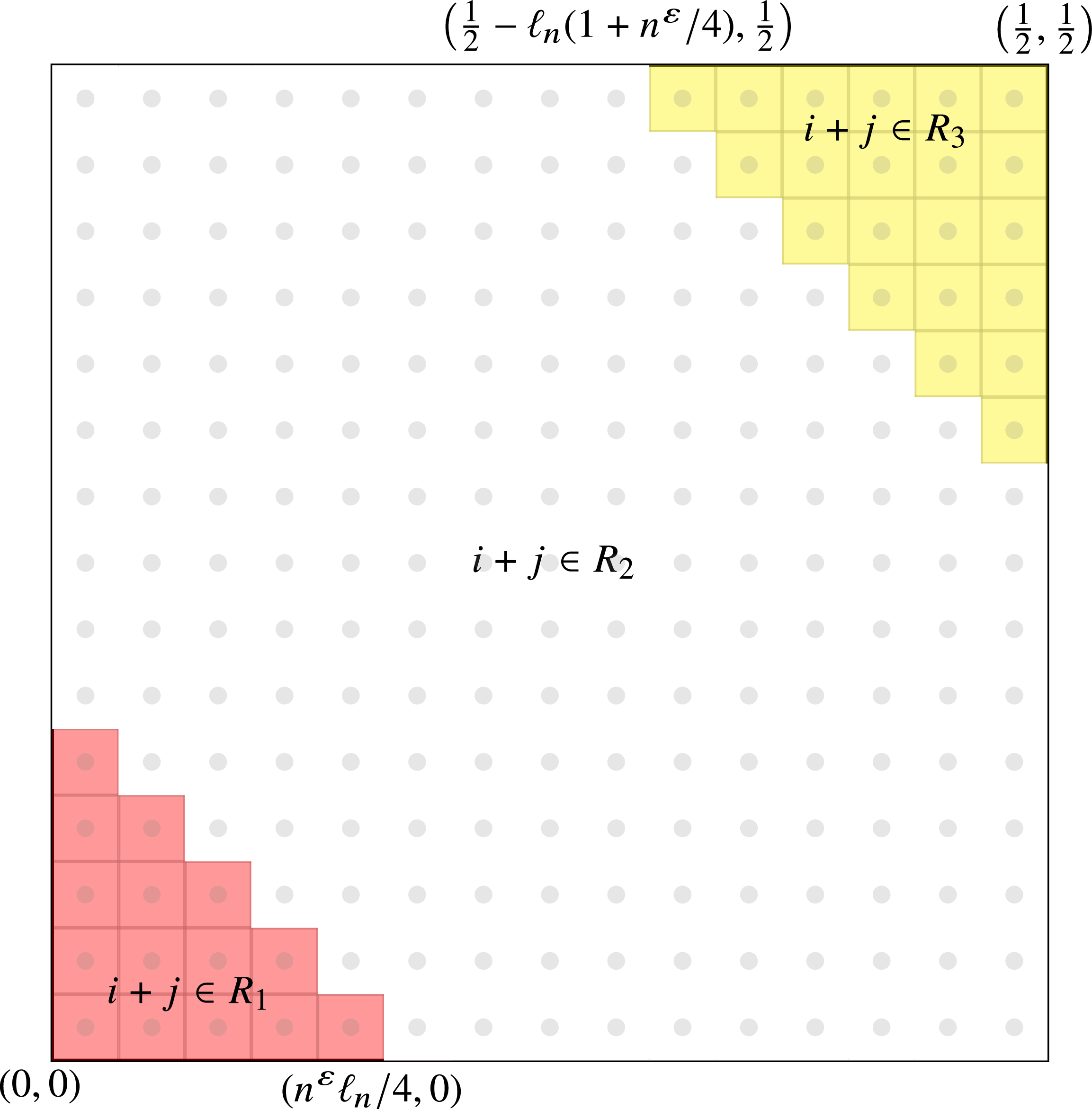
, we split
 $\big[0,\frac12\big]^2$
into three regions; see Figure 2 for an illustration. Fix
 $\varepsilon \in \big(0, \frac13\big)$
. In the first region (the red region in Figure 2), we construct many monotone increasing paths from (0,0) and ending at a point close to the diagonal
 $x+y = (4\sqrt{2})^{-1}n^\varepsilon r_n$
. The monotone paths in this region are such that all edges have labels that are at most
 $\frac14$
, and the label of the mth edge in each path falls in an interval
 $T_m \subset [0,1]$
with
 $|T_m| \approx n^{-\varepsilon}$
. The size of each interval
 $T_m$
is generous, and this generosity is such that, if continued for too long, we would run out of admissible labels before reaching
 $\big(\frac12,\frac12\big)$
. Therefore, in the second region (the white region in Figure 2), we build onto the paths constructed in the first region, if possible, along edges whose labels are more restricted, i.e. ranging from
 $\frac14$
to
 $\frac34$
, and falling in intervals of length
 $\approx n^{-1/3}$
. This construction is such that, with high probability, at least one of the paths from the first region can be extended to have an endpoint close to the diagonal
 $x+y = 1 - (4\sqrt{2})^{-1} r_n(1 + n^\varepsilon/4)$
. In the third region (the yellow region in Figure 2), we proceed similarly to the first region, being generous once again with the edge labels. By a symmetric argument, the path which reached the diagonal
 $x+y = 1 - (4\sqrt{2})^{-1}r_n(1 + n^\varepsilon/4)$
can be extended to a path with endpoint at the point
 $\big(\frac12,\frac12\big)$
. Since the number of vertices of
 $\mathcal{X}_n$
lying in a given region of
 $[0,1]^2$
with area
 $((4\sqrt{2})^{-1}r_n)^2$
is concentrated around its mean,
 $N = (C^2/32)n^{1/3}$
, to formalize this argument it is convenient to frame the construction in terms of an inhomogeneous directed percolation model on the dual grid lattice where the directed edges in the percolation model are open with probabilities given by (3.3).
The intervals
 $R_1, R_2, R_3$
should be thought of as indicating ‘regions’ in the grid in the sense that if, for example,
 $i+j\in R_1$
, then
 $\square_{i,j}$
is a vertex in the portion of the grid which is highlighted in red (and similarly
 $\square_{i,j}$
such that
 $i+j\in R_2$
is in white, and
 $\square_{i,j}$
for
 $i+j\in R_3$
in yellow).

3.1. From temporal graph to directed percolation on the dual grid lattice
Without loss of generality, assume that
 $((4\sqrt{2})^{-1}r_n)^{-1}, (2(4\sqrt{2})^{-1}r_n)^{-1} \in \mathbb{N}$
. Partition
 $\big[0,\frac12\big]^2$
into boxes of side-length
 $\ell_n = (4\sqrt{2})^{-1}r_n$
. Let
 $b_n = (2\ell_n)^{-1}-1$
and, for
 $i,j\in [b_n]_0\,:\!=\,\{0,1,\dots,b_n\}$
, let
 \begin{equation} \square_{i,j} := [i\ell_n, (i+1)\ell_n]\times [j\ell_n, (j+1)\ell_n],\end{equation}
so that by our choice for
 $\ell_n$
, for
 $v\in \mathcal{X}_n\cap \square_{i,j}$
and
 $u\in \mathcal{X}_n\cap \square_{i',j'}$
with
 \begin{align*}(i',j')\in \{(i+1,j), (i-1,j), (i,j+1), (i, j-1)\},\end{align*}
we hace
 ${\mathbb P}\{(u,v)\in E(G_n)\}=\alpha$
.
In this section we map the construction of a temporal path between the points (0, 0) and
 $\big(\frac12,\frac12\big)$
to a directed percolation on the dual grid lattice
 $\mathbb{L}_n = (\mathbb{V}_n,\mathbb{E}_n)$
with vertex set
 $\mathbb{V}_n = \{\square_{i,j} \colon i,j\in [b_n]_0\}$
and directed edge set
 $\mathbb{E}_n$
being the union of the sets
 \begin{align*} \{(\square_{b_n,j}, \square_{b_n, j+1}) & \colon j\in [b_n - 1]_0\}, \\ \{(\square_{i,b_n}, \square_{i+1, b_n}) & \colon i\in [b_n-1]_0\}, \\ \{(\square_{i,j}, \square_{i+1,j}), (\square_{i,j}, \square_{i,j+1}) & \colon i,j\in [b_n-1]_0\}.\end{align*}
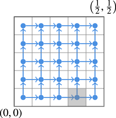
See Figure 3 for an illustration of
 $\mathbb{L}_n$
.
Directed grid lattice with
 $\ell_n = 1/10$
with vertices and directed edges in blue. The filled square highlights vertex
 $\square_{0,3}$
.

The percolation on the finite probability space
 $(\Omega, \mathbb{P}, {\mathcal{P}(\Omega)})$
has configuration space
 $\Omega = \{0,1\}^{\mathbb{E}_n}$
where, for
 $\omega\in \Omega$
and
 $\vec{e}\in \mathbb{E}_n$
,
 $\omega(\vec{e}) = 1$
denotes the directed edge
 $\vec{e}$
being open. For any
 $\omega\in \Omega$
, we say that the vertex
 $\square_{i,j}\in \mathbb{V}_n$
is connected to vertex
 $\square_{k,l}$
, denoted
 $\square_{i,j}\rightarrow \square_{k,l}$
, if there exists an open path in
 $\mathbb{E}_n$
from
 $\square_{i,j}$
to
 $\square_{k,l}$
. That is, if there exists a sequence of open directed edges
 $\vec{e}_0 = (\square_{i,j}, \square_{i_0,j_0})$
,
 $\vec{e}_1 = ( \square_{i_0,j_0}, \square_{i_1,j_1})$
, …,
 $\vec{e}_m = ( \square_{i_m-1,j_m-1}, \square_{k,l})\in \mathbb{E}_n$
.
Informally, the idea of the proof of Proposition 3.1 is to map the construction of a temporal random geometric graph
 $\mathcal{G}_n = (G_n, (\tau_e)_{e\in E(G_n)})$
to a directed percolation of
 $\mathbb{L}_n$
. Fix
 $\varepsilon \in \big(0,\frac13\big)$
. This directed percolation model is such that for
 $i+j\in R_1\cup R_3$
, an edge
 $(\square_{i,j}, \square_{i',j'})\in \mathbb{E}_n$
is open if, in
 $\mathcal{G}_n$
, for each vertex
 $u\in \mathcal{X}_n\cap\square_{i,j}$
there exists a vertex
 $v\in\mathcal{X}_n\cap\square_{i',j'}$
such that the time-stamp
 $\tau_{uv}$
falls in a certain range
 $T_{i+j} \subset [0,1]$
, with
 $|T_{i+j}| \approx n^{-\varepsilon}$
. Crucially, if
 $i+j\in R_2$
, then an edge
 $(\square_{i,j}, \square_{i',j'})\in \mathbb{E}_n$
is open if, in
 $\mathcal{G}_n$
, for a fixed vertex
 $u\in \mathcal{X}_n\cap \square_{i,j}$
there exists a vertex
 $v\in\mathcal{X}_n\cap \square_{i',j'}$
such that
 $\tau_{uv}\in T_{i+j}\subset [0,1]$
with
 $|T_{i+j}| \approx n^{-1/3}$
.
We define the ranges
 $(T_{i+j})_{i,j}$
as follows. For
 ${c > 0}$
,
 $d \in \mathbb{R}$
, and
 $(a,b]\subset \mathbb{R}$
, we write
 $d+c(a,b]$
for
 $(d+ca, d+cb]$
. Then, taking n sufficiently large, for all
 $m \in [b_n]_0$
, let
 \begin{align} T_{m} := \begin{cases} \bigg(\dfrac{m}{n^\varepsilon}, \dfrac{m+1}{n^{\varepsilon}}\bigg], & m\in R_1, \\[12pt] \dfrac{1}{4} + \dfrac{C}{8\sqrt{2}\,}\bigg(\dfrac{1}{n^{1/3}}\bigg(m - \dfrac{n^\varepsilon}{4}\bigg), \dfrac{1}{n^{1/3}}\bigg(m - \dfrac{n^\varepsilon}{4} + 1\bigg)\bigg], & {m\in R_2}, \\[12pt] 1 - \dfrac{2b_n {+ 1}}{n^{\varepsilon}} + \bigg(\dfrac{m}{n^\varepsilon}, \dfrac{m+1}{n^\varepsilon}\bigg], & m \in R_3, \end{cases}\end{align}
where
 $R_1 = [0, n^{\varepsilon}/4)$
,
 $R_2 = [n^{\varepsilon}/4, 2b_n -n^{\varepsilon}/4)$
, and
 $R_3 = [2b_n -n^{\varepsilon}/4, 2b_n]$
. See Figure 2 for an illustration.
Remark 3.1. The sizes of the regions in (3.2) are chosen specifically to work well with the number of edges in
 $\mathcal{G}_n$
that have one endpoint in
 $\square_{i,j}$
and another in
 $\square_{i+1,j}\cup \square_{i,j+1}$
. More specifically, given
 $\mathcal{X}_n$
, the number of edges between a fixed vertex in
 $\mathcal{X}_n\cap \square_{i,j}$
and vertices in
 $\mathcal{X}_n\cap \square_{i+1,j}$
with time-stamp in
 $T_{i,j}$
has distribution Binomial
 $(|\mathcal{X}_n\cap\square_{i+1,j}|,{\alpha}|T_{i+j}|)$
. Since
 $|\mathcal{X}_n \cap \square_{i+1,j}| \stackrel{\mathrm{d}}{=} \mathrm{Binomial}(n,\mathrm{vol}(\square_{i+1,j}))$
, the number of points in
 $\mathcal{X}_n\cap\square_{i+1,j}$
is highly concentrated around its mean,
 $n\cdot\mathrm{vol}(\square_{i+1,j})$
. This implies that if
 $i+j\in R_2$
, then in expectation a constant number of the edges between a fixed vertex in
 $\mathcal{X}_n\cap \square_{i,j}$
and vertices in
 $\mathcal{X}_n\cap (\square_{i+1,j}\cup \square_{i,j+1})$
have time-stamp in
 $T_{i+j}$
. On the other hand, if
 $i+j\in R_1 \cup R_3$
, then the expected number of such edges with time-stamps in
 $T_{i+j}$
is of the order of
 $n^{1/3 - \varepsilon}$
.
We note that, for all i, j, the number of vertices of
 $\mathcal{G}_n$
lying in a given box,
 $\square_{i+1,j}$
, i.e.
 $|\mathcal{X}_n\cap\square_{i+1,j}|$
, is concentrated around its mean
 $N = n \cdot \mathrm{vol}(\square_{i+1,j}) = (C^2/32)n^{1/3}$
. Fix
 $t, t'\in (0,1)$
such that
 $(1+t)N, (1-t')N\in \mathbb{N}$
. Note that later we will work on the high-probability event that
 $|\mathcal{X}_n\cap\square_{i+1,j}| \in [(1-t')N, (1+t)N]$
; see (3.7). Let
 $(B_{\vec{e}})_{\vec{e}\in \mathbb{E}_n}$
be independent random variables satisfying
 $B_{\vec{e}} \stackrel{\mathrm{d}}{=} \text{Binomial}((1-t')N, \alpha|T_{i+j}|)$
. We consider the directed percolation model with edges
 $\vec{e} = (\square_{i,j}, \square_{i',j'})\in \mathbb{E}_n$
open independently with probability
 $p_{\vec{e}}$
, where
 \begin{equation} p_{\vec{e}} := \begin{cases} {\mathbb P}\{B_{\vec{e}} \geq 1 \}^{(1+t)N} & \text{if } i+ j \in R_1 \cup R_3, \\ {\mathbb P}\{B_{\vec{e}} \geq 1 \} & \text{if } i+j \in R_2. \end{cases}\end{equation}
We will denote the law of the directed percolation model by
 $\mathbb{P}$
.
Lemma 3.1. Let
 $\varepsilon \in \big(0,\frac13\big)$
with
 $n^{\varepsilon}/4\in \mathbb{N}$
. The probability of having an open path from
 $\square_{0,0}$
to every box
 $\square_{i,j}$
with
 $i+j = n^{\varepsilon}/4$
in our directed percolation model is bounded from below by
 \begin{equation*} \mathbb{P}\Bigg\{\bigcap_{i+j = {n^\varepsilon}/{4}}\{\square_{0,0} \to \square_{i,j}\}\Bigg\} \geq 1 - \exp(\!-\Omega(n^{1/3 -\varepsilon})). \end{equation*}
Proof. For all
 $\vec{e}\in \mathbb{E}_n$
such that
 $\vec{e} = (\square_{i,j}, \square_{i',j'})$
with
 $i+j < n^\varepsilon/4$
, we have that
 $|T_{i+j}|=n^{-\varepsilon}$
and so the corresponding
 $B_{\vec{e}}$
are independent and identically distributed (i.i.d.) Binomial
 $((1-t')N,\alpha n^{-\varepsilon})$
-distributed random variables. Therefore, recalling that
 $N = (C^2/32)n^{1/3}$
, we obtain that
 \begin{align} p_{\vec{e}} = \mathbb{P}\{B_{\vec{e}} \ge 1\}^{(1+t)N} & = (1 - \mathbb{P}\{B_{\vec{e}} < 1\})^{(1+t)N} \nonumber \\ & \ge 1 - (1+t)N\cdot\mathbb{P}\{B_{\vec{e}} < 1\} \nonumber \\ & \geq 1-(1+t)N\exp\bigg[{-}\frac{\alpha}{n^\varepsilon}(1-t')N\bigg] = 1 - \exp[-\Omega(n^{1/3 - \varepsilon})]. \end{align}
Each edge
 $\vec{e}\in \mathbb{E}_n$
is open independently with probability
 $p_{\vec{e}}$
, and the events
 $\{\square_{0,0}\rightarrow \square_{i,j}\}_{i,j}$
are increasing in
 $\Omega = \{0,1\}^{\mathbb{E}_n}$
. Therefore, by the Fortuin–Kasteleyn–Ginibre inequality (see, e.g., [Reference Janson, Luczak and Rucinski10, Theorem 2.12]),
 \begin{equation*} \mathbb{P}\Bigg\{\bigcap_{i+j = {n^\varepsilon}/{4}}\{\square_{0,0} \to \square_{i,j}\}\Bigg\} \ge \prod_{i+j = {n^\varepsilon}/{4}}\mathbb{P}\{\square_{0,0}\rightarrow \square_{i,j}\} \ge \prod_{i+j = {n^\varepsilon}/{4}} p_{\vec{e}}^{n^\varepsilon/4}, \end{equation*}
where for the second inequality we have used the fact that
 $\mathbb{P}\{\square_{0,0}\rightarrow \square_{i,j}\}$
is at least the probability that a single path of length
 $n^\varepsilon/4-1$
is open. Combining this with (3.4) and the inequality
 $(1-x)^k\ge 1-xk$
for
 $x\in (0,1)$
yields the result.
Lemma 3.2. Let
 $\varepsilon\in\big(0,\frac13\big)$
with
 $n^{\varepsilon}/4\in \mathbb{N}$
. Then the probability of having an open path from a box
 $\square_{i,j}$
with
 $i+j = n^{\varepsilon}/4$
to a box
 $\square_{k,l}$
with
 $k+l = 2b_n-n^{\varepsilon}/4$
in our directed percolation model can be bounded from below by
 \begin{equation*} \mathbb{P}\Bigg\{\bigcup_{i+j = {n^{\varepsilon}}/{4}}\,\bigcup_{k+l = 2b_n - {n^\varepsilon}/{4}} \{\square_{i,j}\rightarrow \square_{k,l}\}\Bigg\} \geq 1 - \exp[\!-\Omega(n^{\varepsilon} \wedge n^{1/3-\varepsilon})]. \end{equation*}
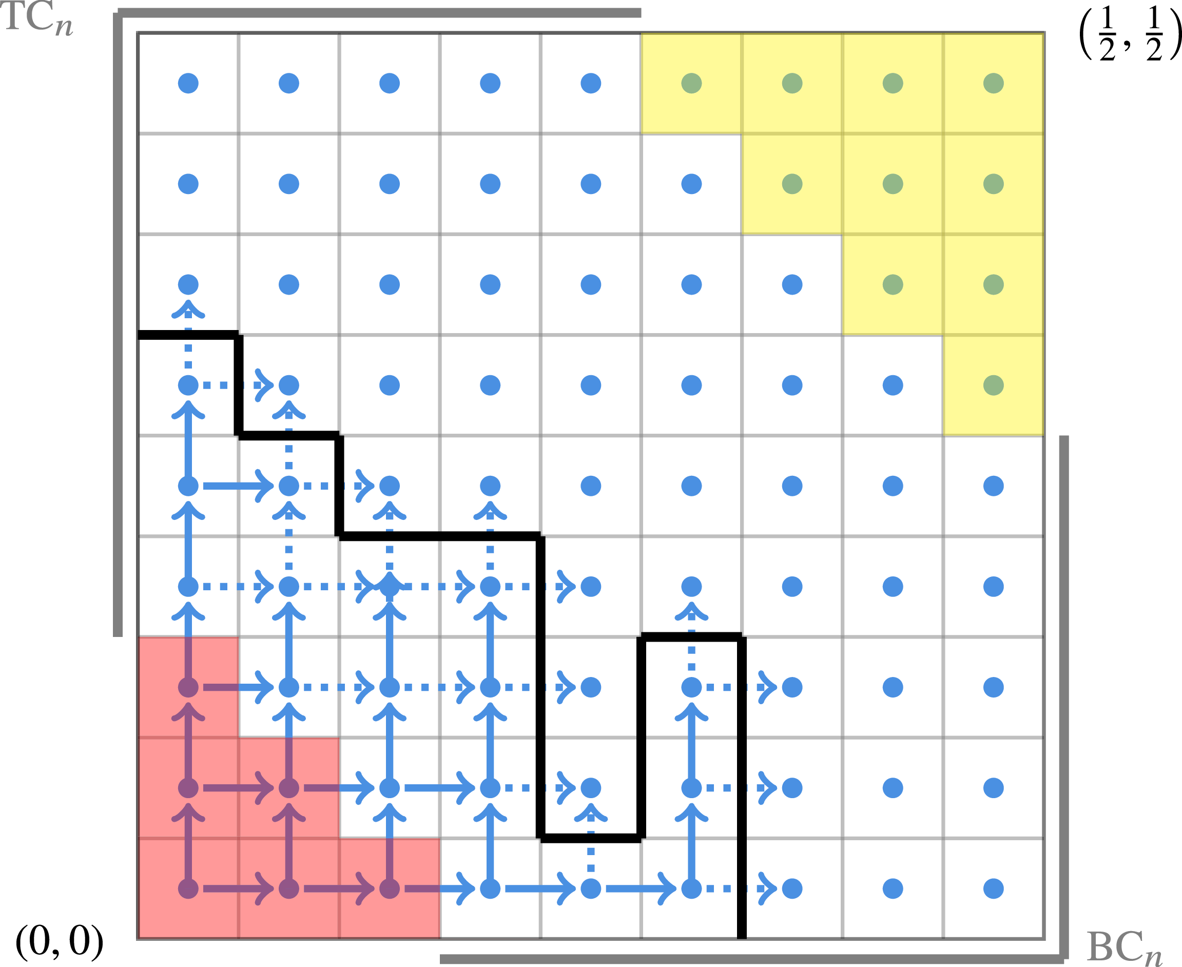
The connected component containing
 $\square_{0,0}$
. Open edges are drawn as solid blue arrows while closed edges are drawn as dotted blue arrows. In black is the boundary of the connected component containing
 $\square_{0,0}$
as a path in the lattice with mesh size
 $\ell_n$
. The bold-face grey lines border the regions
 $\mathrm{TC}_n$
and
 $\mathrm{BC}_n$
.

Proof. We condition on the event
 $\mathcal{E}_n = \bigcap_{i+j = {n^\varepsilon}/{4}}\{\square_{0,0} \rightarrow \square_{i,j}\}$
, which, by Lemma 3.1, occurs with probability
 $1 - \exp[-\Omega(n^{1/3 - \varepsilon})]$
. On this event, if there is no open path between
 $\{\square_{i,j}\colon i+j = n^\varepsilon/4\}$
and
 $\{\square_{k,l}\colon k+l = 2b_n - n^\varepsilon/4\}$
, then the connected component containing
 $\square_{0,0}$
and the vertices
 $\{\square_{i,j}\colon i+j = n^\varepsilon/4\}$
has a boundary which can be represented as a path in the lattice (rather than in the dual grid lattice) with mesh size
 $\ell_n$
, with one endpoint in the top left-hand corner region of the unit square,
 \begin{align*} \mathrm{TC}_n := \{(0,j\ell_n) \colon j \in \{n^\varepsilon/4,\dots, b_n + 1\}\} \cup \{(i\ell_n, {1}) \colon i\in \{0,\dots,b_n-n^\varepsilon/4\}\}, \end{align*}
and the other in the bottom right-hand corner of the unit square,
 \begin{align*} \mathrm{BC}_n := \{({1},j\ell_n) \colon j \in \{0,\dots,b_n-n^\varepsilon/4\}\} \cup \{(i\ell_n,0) \colon i \in \{n^\varepsilon/4,\dots,b_n+1\}\}. \end{align*}
See Figure 4 for an illustration.
Let
 $P^{(i,j)}_n$
be the number of paths which form a boundary in the percolation model with one endpoint being the point
 $(i\ell_n,j\ell_n)\in \mathrm{TC}_n$
and the other endpoint being in
 $\mathrm{BC}_n$
. Then
 \begin{equation} \mathbb{P}\Bigg\{\bigcup_{i+j = {n^\varepsilon}/{4}}\,\bigcup_{k+l = 2b_n - {n^\varepsilon}/{4}} \{\square_{i,j}\rightarrow \square_{k,l}\} \mid \mathcal{E}_n\Bigg\} \ge 1 -\sum_{(i\ell_n,j\ell_n)\in \mathrm{TC}_n}\mathbb{P} \big \{P^{(i,j)}_n \ge 1 \big\}. \end{equation}
To prove Lemma 3.2 it remains to show that the right-hand side of the above inequality can be bounded from below by
 $1 - \exp[-\Omega(n^{\varepsilon})]$
. To this end, let
 $(i\ell_n,j\ell_n)\in \mathrm{TC}_n$
. We use the first-moment method to bound
 $\mathbb{P}\{P^{(i,j)}_n \ge 1\}$
. Each path that could form a boundary for the directed percolation has length
 $m\in \{n^{\varepsilon}/2,\dots, 2b_n(b_n +1) \}$
, where we note that the upper bound is the total number of edges in the lattice and
 $2b_n(b_n+1) = ({16}/{C^2})n^{2/3}-({4\sqrt{2}}/{C})n^{1/3}$
. Lastly, in order for such a path to represent a boundary of the connected component, at least one half of its edges must intersect closed edges of
 $\mathbb{L}_n$
(viewing the path as from
 $\mathrm{TC}_n$
to
 $\mathrm{BC}_n$
, the edges that step down or right must intersect closed edges of
 $\mathbb{L}_n$
); again, see Figure 4. By (3.3) and (3.2), the directed edges intersecting this path are each closed independently with probability
 $1 - {\mathbb P}\{B^{(n)} \ge 1\}$
, where
 $B^{(n)}$
is a Binomial
 $((1-t')N,\alpha|T_{n^\varepsilon/4}|)$
-distributed random variable where
 \begin{align*}|T_{n^{\varepsilon}/4}| = \frac{C}{8\sqrt{2}n^{1/3}}.\end{align*}
Since
 $N = ({C^2}/{32})n^{1/3}$
, it follows that
 \begin{align*} \mathbb{E}\{B^{(n)}\} = \frac{\alpha (1-t')CN}{8\sqrt{2}n^{1/3}} = \frac{\alpha(1-t')C^3n^{1/3}}{32\cdot 8\sqrt{2}n^{1/3}} = \frac{\alpha(1-t')C^3}{256\sqrt{2}}. \end{align*}
It follows that, for all
 $\delta > 0$
, for n sufficiently large,
 \begin{align*} {\mathbb P}\{B^{(n)} \ge 1\} \ge {\mathbb P}\bigg\{\mathrm{Poisson}\bigg({\frac{\alpha(1-t')C^3}{256\sqrt{2}}}\bigg) \ge 1\bigg\} - \delta, \end{align*}
and so
 \begin{equation*} 1 - {\mathbb P}\{B^{(n)} \ge 1\} \leq \exp\bigg[{-}\frac{\alpha(1-t')C^3}{256\sqrt{2}}\bigg] + \delta. \end{equation*}
Let
 $\delta > 0$
. Notice that to construct a boundary path edge by edge starting from a point in
 $\mathrm{TC}_n$
, at each step there are at most three possibilities for the direction of the next added edge. Therefore, we obtain that, for sufficiently large n,
 \begin{align*} \mathbb{E}\big\{P^{(i,j)}_n \big\} & \leq \sum_{m=n^{\varepsilon}/2}^{2b_n(b_n + 1)}3^m(1 - {\mathbb P}\{B \ge 1\})^{\lfloor m/2\rfloor} \\ & \leq \sum_{m=n^{\varepsilon}/2}^{4b_n^{2}}3^m\bigg(\exp\bigg[{-}\frac{\alpha(1-t')C^3}{256\sqrt{2}}\bigg] + \delta\bigg)^{\lfloor m/2\rfloor} \\ & \leq \ell_n^{-2}\bigg(10\exp\bigg[{-}\frac{\alpha(1-t')C^3}{256\sqrt{2}}\bigg]\bigg)^{n^{\varepsilon}/4}, \end{align*}
where the final inequality follows from taking
 $\delta>0$
sufficiently small. Taking
 $C>0$
sufficiently large, so that
 \begin{equation*} 10\exp\bigg[{-}\frac{\alpha(1-t')C^3}{256\sqrt{2}}\bigg] < {\mathrm{e}}^{-4}, \end{equation*}
we obtain that
 $\mathbb{E}\{P^{(i,j)}_n\} = \exp[-\Omega(n^{\varepsilon})]$
. The result then follows from (3.5) by an application of Markov’s inequality and the fact that
 $\#\{(i\ell_n, j\ell_n) \in \mathrm{TC}_n\} = O(\ell_n^{-1}) = O(n^{1/3})$
.
3.2. Proof of Proposition 3.1.
In this subsection we show how Lemmas 3.1 and 3.2 imply that, for
 $\varepsilon \in \big(0,\frac19\big)$
,

for
 $(\mathcal{G}_n)_{n\geq 1}$
as in Proposition 3.1, where we work with a modified point process obtained by adding the points (0,0) and
 $\big(\frac12,\frac12\big)$
to
 $\mathcal{X}_n$
. To see why Proposition 3.1 follows from (3.6), note that the maximal distance between two vertices in
 $\mathcal{G}_n$
is
 $\sqrt{2}/2$
, for instance between (0, 0) and
 $\big(\frac12,\frac12\big)$
. Since we are working on the torus
 $[0,1]^2$
, the same proof construction can be used for any pair of points
 $(x,y), (x',y') \in \mathcal{X}_n$
by translating and/or the first and third regions (highlighted in red and yellow in Figure 5) such that they start at (x, y) and (x
′, y
′) respectively, and appropriately shrinking the second region (the white region in Figure 5), while keeping the box side-length
 $\ell_n = (4\sqrt{2})^{-1}r_n$
as before. If the first and third regions overlap (and so there is no white region in Figure 5), we shrink the first and third regions appropriately while keeping the same box side-length as in the original construction. A union bound over all possible pairs of vertices then gives
 , proving Proposition 3.1 for
 $d=2$
.
Illustration of the construction in Proposition 3.1. The red, white, and yellow regions, shown (a) in the original unshifted position, and (b) rotated and translated to an arbitrary pair of points (x, y), (x
′, y
′) on the torus, with the same grid box size
 $\ell_n$
throughout.

Proof of Proposition
3.1 with
 $d = 2$
. As discussed above, to prove Proposition 3.1, it suffices to prove (3.6). Recall
 $(\square_{i,j})_{i,j}$
from (3.1). We begin by defining
 $A_n$
as the event that the number of vertices in each box
 $\square_{i,j},$
is well concentrated. More precisely, for
 $t, t'\in (0,1)$
let
 \begin{equation} A_n = A_n(t, t') := \Big\{\max_{i,j}\big||\mathcal{X}_n \cap \square_{i,j}| - N\big| < (t \vee t')N\Big\}, \end{equation}
recalling that
 $|\mathcal{X}_n \cap \square_{i,j}|$
is a Binomial
 $(n,\text{vol}(\square_{0,0}))$
random variable, and
 $N = n \text{vol}(\square_{0,0}) = (C^2/32)n^{1/3}$
. By [Reference Lavrov and Loh11, Corollary 2.3], for all
 $t\in (0,1)$
, for
 $n \ge 1$
,
 \begin{equation} \mathbb{P} \big\{A_n^{\mathrm{c}} \big\} \le \frac{16n^{2/3}}{C^2}\exp\bigg[{-}\frac{(C\,t \vee t')^2}{96}n^{1/3}\bigg] = \exp[-\Omega(n^{1/3})]. \end{equation}
We therefore focus on proving that
 can be bounded from below by the right-hand side of (3.6) for the remainder of this section. We lower bound this probability by that of having a temporal path from (0, 0) to
 $\big(\frac{1}{2},\frac{1}{2}\big)$
using only edges xy satisfying
 $x\in \mathcal{X}_n \cap \square_{i,j}$
,
 $y \in \mathcal{X}_n \cap (\square_{i+1,j} \cup \square_{i,j+1})$
, and
 $\tau_{xy}\in T_{i,j}$
. Observe that by our choice of box side-length
 $\ell_n = (4\sqrt{2})^{-1}r_n$
we have that an edge xy with
 $x\in \mathcal{X}_n \cap \square_{i,j}$
,
 $y \in \mathcal{X}_n \cap (\square_{i+1,j} \cup \square_{i,j+1})$
exists with probability
 $\alpha$
. Further remark that, for all
 $i,j \in [b_n]_0$
and
 $\vec{e} = (\square_{i,j}, \square_{i',j'}) \in \mathbb{E}_n$
,
 \begin{align*} & {\mathbb P}\{\text{for all } x\in \mathcal{X}_n \cap \square_{i,j} \text{ there exists } y \in \mathcal{X}_n \cap \square_{i',j'} \text{ such that } xy \in E(G_n), \tau_{xy} \in T_{i+j} \mid A_n\} \\ & \qquad \geq {\mathbb P}\Bigg\{\bigcap_{k\in [(1+t)N]}\{B_{\vec{e}, k} \geq 1\}\Bigg\}, \end{align*}
where
 $(B_{\vec{e}, k})_{k\geq 1}$
are i.i.d.
 $\text{Binomial}((1-t')N, \alpha|T_{i,j}|)$
-distributed random variables. Indeed, note that, for any fixed
 $x\in \mathcal{X}_n \cap \square_{i,j} $
,
 \begin{equation*} {\mathbb P}\{\text{there exists } y \in \mathcal{X}_n \cap \square_{i',j'} \text{ such that } xy \in E(G_n), \tau_{xy} \in T_{i+j} \mid A_n\} \geq {\mathbb P}\{B_{\vec{e}} \geq 1\}. \end{equation*}
Finally, we will ensure that if we can reach some vertex in the final box
 $\square_{b_n, b_n}$
with a temporal path using only time-stamps in
 $[0,1-n^{-\varepsilon}]$
, then we can complete the temporal path from (0, 0) to
 $\big(\tfrac{1}{2},\tfrac{1}{2}\big)$
using two further edges. To be precise, on the event
 $A_n$
, given
 $x\in \mathcal{X}_n \cap \square_{b_n, b_n}$
, the probability of having a temporal path from x to
 $\big(\frac{1}{2},\frac{1}{2}\big)$
only using edges with time-stamps in
 $(1-n^{-\varepsilon}, 1]$
is bounded from below by the probability of having
 $n^{1/3-2\varepsilon}$
vertices
 $y\in \mathcal{X}_n \cap \square_{b_n, b_n}$
such that
 $xy \in E(G_n)$
and
 $\tau_{xy}\in (1-n^{-\varepsilon}, 1 - n^{-\varepsilon}/2]$
and such that one of these y satisfies
 $y\big(\frac{1}{2},\frac{1}{2}\big) \in E(G_n)$
and
 $\tau_{y({1}/{2},{1}/{2})}\in (1 - n^{-\varepsilon}/2, 1]$
. This probability can further be bounded from below by
 \begin{equation} {\mathbb P}\{\text{Binomial}((1-t')N,\alpha n^{-\varepsilon}/2) \geq n^{1/3-2\varepsilon}\} \times {\mathbb P}\{\text{Binomial}(n^{1/3-2\varepsilon},\alpha n^{-\varepsilon}/2) \geq 1\}. \end{equation}
The mean of the Binomial in the first probability is of the order of
 $n^{1/3 - \varepsilon}$
. Thus, by a Chernoff bound (see [Reference Janson, Luczak and Rucinski10, Theorem 2.1]), this probability is at least
 $1- \exp[-\Omega(n^{1/3-\varepsilon})]$
. The second term in (3.9) equals
 $1-(1- \alpha n^{-\varepsilon}/2)^{n^{1/3 - 2\varepsilon}} = 1 - \exp[\!-\Omega(n^{1/3 - 3\varepsilon})]$
. Putting everything together, on the event
 $A_n$
, given
 $x\in \mathcal{X}_n \cap \square_{b_n, b_n}$
, the probability of having a temporal path from x to
 $\big(\frac{1}{2},\frac{1}{2}\big)$
only using edges with time-stamps in
 $(1-n^{-\varepsilon}, 1]$
is bounded from below by
 $1-\exp[\!-\Omega(n^{1/3 - 3\varepsilon})]$
.
From this, we can see that

Since the edges
 $\vec{e}\in \mathbb{E}_n$
are open independently,
 $\mathbb{P}\{\square_{0,0} \to \square_{b_n,b_n}\}$
can be bounded from below by
 \begin{align} & \mathbb{P}\Bigg\{\bigcap_{i+j = {n^{\varepsilon}}/{4}-1}\{\square_{0,0} \to \square_{i,j}\}\Bigg\} \\[-8pt] \nonumber \end{align}
 \begin{align} &\! \times \mathbb{P}\Bigg\{\bigcup_{i+j = {n^{\varepsilon}}/{4}-1}\,\bigcup_{k+l = 2b_n - n^{\varepsilon}/4} \{\square_{i,j} \to \square_{k,l}\}\Bigg\} \\[-8pt] \nonumber \end{align}
 \begin{align} &\! \times \mathbb{P}\Bigg\{\bigcap_{i + j = 2b_n - n^{\varepsilon}/4}\{\square_{i,j} \to \square_{b_n,b_n}\}\Bigg\}. \end{align}
Lemmas 3.1 and 3.2 yield a lower bound for (3.11) and (3.12). Further, since the time-stamp ranges in the lower-left and upper-right triangle regions,
 $\{\square_{i,j}\colon i+ j \leq n^{\varepsilon}/4-1\}$
and
 $\{\square_{i,j}\colon i+ j \geq 2b_n - n^{\varepsilon}/4\}$
respectively, and all satisfy
 $|T_{i+j}| = n^{-\varepsilon}$
, we can argue by symmetry that the lower bound in Lemma 3.1 also holds for (3.13), giving
 \begin{equation*} \mathbb{P}\{\square_{0,0} \to \square_{b_n, b_n}\} \geq 1 - \exp[\!-\Omega(n^{1/3-\varepsilon})] - \exp[\!-\Omega(n^{\varepsilon})]. \end{equation*}
Together with (3.10) and (3.8), we conclude (3.6), proving Proposition 3.1.
3.2.1. Extension to dimension
$d > 2$
.

The proof of Proposition 3.1 in dimension
 $d > 2$
can be deduced from the dimension
 $d = 2$
case. Similarly to the case
 $d=2$
, it suffices to construct a likely path from the furthest possible separated points on the torus
 $[0,1]^d$
, namely
 $\vec{0},\smash{\vec{{1}/{2}}}$
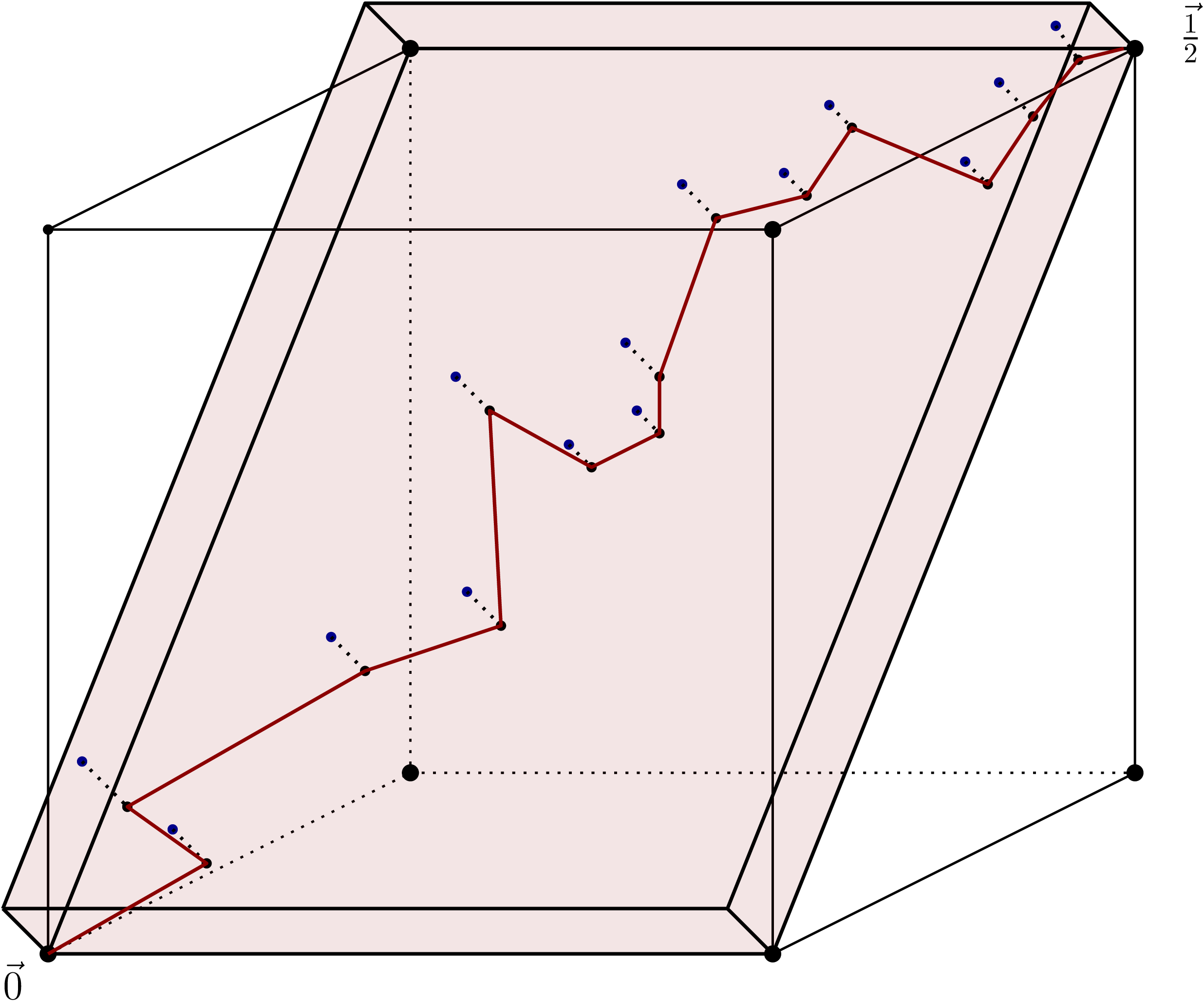
, and then conclude by a union bound. For such a path, we only consider points that are inside a slab of width
 $r_n/2$
. More precisely, in this slab the points
 $\vec{0}, \smash{\vec{{1}/{2}}}$
are the opposite corners of a rotated copy
 $\smash{[0,{\sqrt{d}}/{2\sqrt{2}}]^2 \times \{0\}^{d-2}}$
. This slab has volume of order
 $r_n^{d-2}$
, and therefore with high probability the number of points in this region is
 $\Omega(nr_n^{d-2})$
. See Figure 6 for an illustration.
Illustration of the argument for higher dimensions. The aim is to construct a likely path from
 $\vec{0}$
to
 $\smash{\vec{{1}/{2}}}$
using only vertices in the slab shaded in red. When projecting these vertices onto a two-dimensional plane, we can construct a likely path (illustrated in red) following the proof for
 $d=2$
.

We project these points onto a copy of
 $\smash{[0,{\sqrt{d}}/{2\sqrt{2}}]^2}$
and note that, for any two vertices in the slab u, v, if their projections
 $\hat{u}$
and
 $\hat{v}$
are such that
 $\|\hat{u} - \hat{v}\| \le r_n/2$
, then
 $\|u-v\| \le r_n$
and so
 \begin{equation*} {\mathbb P}\{uv\in E(G_n) \mid \mathcal{X}_n\} = K\bigg(\frac{\|u-v\|}{r_n}\bigg) \geq K\bigg(\frac{\|\hat{u} - \hat{v}\|}{r_n/2}\bigg).\end{equation*}
Partitioning the two-dimensional square into boxes of side-length of order
 $r_n \approx n^{-1/(d+1)}$
, the expected number of points in a box
 $\square_{i,j}$
is
 $N = nr_n^{d-2}\cdot \text{vol}(\square_{i,j}) \approx n r_n^d \approx n^{1/(d+1)}$
. With this value of N, the proofs and statements of Lemmas 3.1 and 3.2, and of (3.6), carry over (with slight adjustments of constants), yielding analogous bounds with
 $n^{1/3}$
replaced by
 $n^{1/(d+1)}$
throughout. This proves Proposition 3.1 for all
 $d\geq 2$
.
Acknowledgements
This research was initiated during the Seventeenth Annual Workshop on Probability and Combinatorics at McGill University’s Bellairs Institute in Holetown, Barbados. We thank the Bellairs Institute for its hospitality. We would also like to thank two reviewers for their thorough reading of the paper and for their valuable suggestions.
Funding information
AB was supported by NSF GRFP 2141064 and Simons Investigator Award 622132 to Elchanan Mossel. SD acknowledges the financial support of the CogniGron research center and the Ubbo Emmius Funds (University of Groningen). CK was supported by DFG project 444092244 ‘Condensation in random geometric graphs’ within the priority programme SPP 2265. GL acknowledges the support of Ayudas Fundación BBVA a Proyectos de Investigación Científica 2021 and the Spanish Ministry of Economy and Competitiveness grant PID2022-138268NB-I00, financed by MCIN/AEI/10.13039/501100011033, FSE+MTM2015-67304-P, and FEDER, EU. RM was supported by the EPSRC Centre for Doctoral Training in Mathematics of Random Systems: Analysis, Modelling and Simulation (EP/S023925/1).
Competing interests
There were no competing interests to declare which arose during the preparation or publication process of this article.


 [0,1]2
 R1,R2,R3
 i+j∈R1
 ◻i,j
 ◻i,j
 i+j∈R2
 ◻i,j
 i+j∈R3
 ℓn=1/10
 ◻0,3
 ◻0,0
 ◻0,0
 ℓn
 TCn
 BCn

 ℓn
 0→
 1/2→
 d=2

 Open access

