


1 Introduction
In the Euclidean plane
$\mathbb {R}^{2}$
 , construct the lines
$ {x}={k} $
 for integers
$k$
 . Centre a disc of radius
$r$
 on
$ (S, 0) $
 , where S has a uniform distribution on
$ [0,1] $
 . Let
$ {L} \equiv {L}({r}) $
 be the total chord length from the intersection of the disc with the lines. Let
$ {{F}({\ell })} \equiv {{\mathbb {P}}\{{L} \leq {\ell }\}} $
 be the cumulative distribution function (cdf) for
$L$
 . This article obtains
${F}({\ell })$
 .
Theorem 1.1. For
$ {x} \in {\mathbb {R}} $
 , let

Write
$ {r} = {n} + {s} $
 where
$n$
 is an integer and
$ {s} \in [0,1)$
 . Set
$ {a} = \lfloor -2{s} \rfloor / 2 $
 ,
$ {b} = {a} + 1/2 $
 , and
$ {{u}_{\operatorname {\mathrm {min}}}} = {{u}(-{s})} $
 ,
$ {{u}_{\operatorname {\mathrm {max}}}} = \operatorname {\mathrm {max}}\{ {u}({a}), {u}({b}) \} $
 . Then

where
$c$
 and
$d$
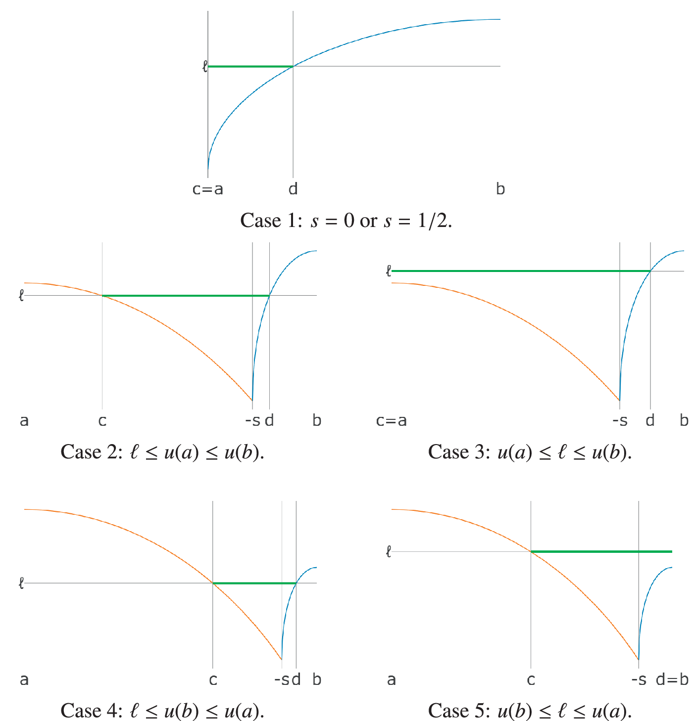
 are specified in the following table (see also Figure 1).

Calculating
${\mathbb {P}}\{{L} \leq {\ell }\}$
 . The orange and blue curves plot
${u}({x})$
 on
$ [{a}, {b}] $
 . The thick green line marks the interval
$ [{c}, {d}] $
 . If
$X$
 follows a uniform distribution on
$ [{a}, {b}] $
 then
$ \{ {X} \in [{c}, {d}] \} \equiv \{ {L} \leq {\ell } \} $
 .

Figure 1 Long description
The figure consists of five panels labeled Case 1 through Case 5. Each panel features a horizontal x-axis with points a, b, c, d, and sometimes minus s. A horizontal reference line is labeled ell. The data is represented by orange and blue curves for the function u of x, and a thick green horizontal line segment representing the interval where u of x is less than or equal to ell.
* Case 1: At the top, a single blue curve rises from c equals a to b. A green line segment extends from the vertical axis at ell to the intersection with the blue curve at d.
* Case 2: Middle left. An orange curve descends to a sharp trough at minus s, where a blue curve then rises. The green line segment spans from c on the orange curve to d on the blue curve.
* Case 3: Middle right. Similar curves to Case 2, but the green line segment is higher, extending from the vertical axis at c equals a across to the blue curve at d.
* Case 4: Bottom left. The orange curve descends and the blue curve rises from a trough at minus s. The green line segment is lower, spanning from c on the orange curve to d on the blue curve.
* Case 5: Bottom right. The green line segment extends from c on the orange curve to the rightmost boundary where d equals b.
Theorem 1.1 adds to the literature of geometric probability, and may have applications in stereology. It will be shown that when
$ {r} \leq 1/2 $
 , Theorem 1.1 agrees with earlier findings on the length of a single random chord [Reference Chiu, Dietrich, Kendall and Mecke1, Equation (1.66)].
2 Proof of Theorem 1.1
Proof. The probability function
${F}({\ell })$
 is constructed by inverse transform sampling: Proposition 2.1 establishes
$ {L} = {{u}({X})} $
 where
$X$
 is uniformly distributed on
$ [{a}, {b}] $
 . To invert
${u}({x})$
 , Propositions 2.4 and 2.5 prove that
${u}({x})$
 is strictly decreasing on
$ [{a}, -{s}] $
 and strictly increasing on
$ [-{s}, {b}] $
 . So
$ \{ {X} \in [{c}, {d}] \} \equiv \{ {L} \leq {\ell } \} $
 , whereby
$ {{\mathbb {P}}\{{L} \leq {\ell }\}} = ( {d} - {c} )/( {b} - {a} ) $
 .
To prove Propositions 2.1, 2.4 and 2.5, first note that
${{u}_{{k}}}({x})$
 is the length of the chord made by the line
$ {x}={k} $
 when it crosses a disc of radius
$r$
 centred on
$ ({x}, 0) $
 .
Proposition 2.1. The total chord length
$L$
 can be realised as
$ {L} = {{u}({X})} $
 where
$X$
 is uniformly distributed on
$ [{a}, {b}] $
 .
Proof. Observe that
${u}({x})$
 is constructed as the total chord length formed by the lines
$ {x}={k} $
 for integers
$k$
 , for a disc of radius
$r$
 centred on
$ ({x}, 0) $
 : the sum is over
${{k} = \lceil {x} - {r} \rceil, \ldots, \lfloor {x} + {r} \rfloor }$
 because lines outside that range will not intersect the disc. Now the lines are at unit spacing, which creates a translation symmetry, whereby
${{{u}({x}+{k})} = {{u}({x})}}$
 for all integers
$k$
 . Moreover, a disc is symmetric in reflection, so
$ {{u}(-{x})} = {{u}({x})} $
 for all real numbers
$x$
 . Thus,
$L$
 is fully characterised by
${u}({X})$
 where
$X$
 is drawn uniformly from an interval that is of width
$ 1/2 $
 and has an integer as one of its boundaries. The interval
$ [{a}, {b}] $
 is one such interval.
To prove monotonicity of
${u}({x})$
 , take the chords in pairs. Within each pair, it will be shown that the shorter chord grows faster than the longer chord shrinks. The following lemma locates the shorter chord within a pair.
Lemma 2.2. Centre a disc of radius
$r$
 on
$ ({x}, 0) $
 . Let
$ {k} \geq 0 $
 and
$ {j} \in {\mathbb {R}} $
 . Then the chord formed by the line
$ {x}={k} $
 is strictly shorter (longer) than the chord formed by the line
$ {x}=-{k}+ {j} $
 if and only if
$ (2{k} - {j})(2{x} - {j}) < 0 \ (\mathrm {respectively,}> \, 0) $
 .
Proof. Since
$ {{{u}_{{k}}}({x})} = 2\sqrt {{r}^2 - ({k} - {x})^2} $
 and
$ {{{u}_{-{k}+{j}}}({x})} = 2\sqrt {{r}^2 - (-{k}+{j} - {x})^2} $
 , the inequality
$ {{{u}_{{k}}}({x})} < {{{u}_{-{k}+{j}}}({x})} $
 holds if and only if
$ ({k} - {x})^2> (-{k}+{j} - {x})^2 $
 . Observe that
 . The result follows.
Henceforth, for any
$ {m} \in {\mathbb {R}} $
 , let
$ {y_{{m}}} \equiv {{y_{{m}}}({x})} = \sqrt {{r}^2 - ({m} - {x})^2} $
 . Note
$ {{y'_{{m}}}} \equiv {{{y'_{{m}}}}({x})} = ({m} - {x}) / {y_{{m}}} $
 . The following lemma will establish whether the net rate of growth for a pair of chords is positive or negative.
Lemma 2.3. Let
$ {k}, {j} \in {\mathbb {R}} $
 . If
$ x < (>) \, {j}/2 $
 and
$ ({k} - {x})({y_{-{k}+{j}}} - {y_{{k}}})> (<) \, 0 $
 then
$ {{y'_{{k}}}} + {{y'_{-{k}+{j}}}}> (<) \, 0 $
 .
Proof. Observe that

Since
$ {y_{{k}}}, {y_{-{k}+{j}}}> 0 $
 , it is sufficient to consider the numerator

Now
$ {x} < {j}/2 $
 if and only if
$ {j} - {x}> {j} - {j}/2 = {j}/2 > {x} $
 , whereby

Conversely, if
$ {x}> {j}/2 $
 then the inequalities are reversed. The result follows.
Monotonicity can now be established, in either direction from
$ -{s} $
 .
Proposition 2.4. The function
${u}({x})$
 is strictly increasing on
$ [-{s}, {b}] $
 .
Proof. It is sufficient to show that
$ {{{u}'}({x})}> 0 $
 for
$ {x} \in (-{s}, {b}) $
 , as the result will follow from
${u}({x})$
 being continuous on
$ [-{s}, {b}] $
 . For
$ 0 \leq {s} < 1 $
 , if
$ {x} \in (-{s}, {b}) $
 then we have
${ {x} + {r}> -{s} + {n} + {s} = {n} }$
 and
$ {x} + {r} < {b} + {n} + {s} \leq {n}+1/2 $
 , therefore
$ \lfloor {x} + {r} \rfloor = {n} $
 . We consider three cases.
-
(1) $ {s} = 0 $
 . If
$ {x} \in (-{s}, {b}) $
, then
$ {x} - {r}> -{s} - {n} - {s} = -{n} $
and
$ {x} - {r} < {b} - {n} - {s} = -{n} + 1/2 $
. Therefore,
$ \lceil {x} - {r} \rceil = -{n} + 1 $
. Thus, $$ \begin{align*} {{u}({x})} = \displaystyle\sum_{{k}=-{n}+1}^{{n}} {{{u}_{{k}}}({x})} = \displaystyle\sum_{{k}=1}^{{n}} ( {{{u}_{{k}}}({x})} + {{{u}_{-{k}+1}}({x})} ). \end{align*} $$Set $ {j} = +1 $
.
-
(2) $ 0 < {s} \leq 1/2 $
. If
$ {x} \in (-{s}, {b}) $
, then
$ {x} - {r}> -{s} - {n} - {s} > -{n}-1 $
and so we have
${ {x} - {r} < {b} - {n} - {s} < -{n} }$
. Therefore,
$ \lceil {x} - {r} \rceil = -{n} $
. Thus, $$ \begin{align*} {{u}({x})} = \displaystyle\sum_{{k}=-{n}}^{{n}} {{{u}_{{k}}}({x})} = {{{u}_{0}}({x})} + {} \displaystyle\sum_{{k}=1}^{{n}} ( {{{u}_{{k}}}({x})} + {{{u}_{-{k}}}({x})} ). \end{align*} $$Set $ {j} = 0 $
.
-
(3) $ 1/2 < {s} < 1 $
. If
$ {x} \in (-{s}, {b}) $
, then
$ {x} - {r}> -{s} - {n} - {s} > -{n}-2 $
and so we have
${ {x} - {r} < {b} - {n} - {s} < -{n}-1 }$
. Therefore,
$ \lceil {x} - {r} \rceil = -{n}-1 $
. Thus, $$ \begin{align*} {{u}({x})} = \displaystyle\sum_{{k}=-{n}-1}^{{n}} {{{u}_{{k}}}({x})} = \displaystyle\sum_{{k}=0}^{{n}} ( {{{u}_{{k}}}({x})} + {{{u}_{-{k}-1}}({x})} ). \end{align*} $$Set $ {j} = -1 $
.


In each case,
$ {b} = {j}/2 $
 and hence
$ {x} < {j}/2 $
 . Moreover,
$ 2{k} - {j}> 0 $
 for each index
$k$
 in the sums. Thus, for each such
$k$
 ,
$ {y_{{k}}} < {y_{-{k}-1}} $
 by Lemma 2.2, hence
$ {{y'_{{k}}}} + {{y'_{-{k}-1}}}> 0 $
 by Lemma 2.3. For case 2, note
$ {{y'_{0}}} = -{x}/{y_{0}}> 0 $
 . The result follows from
$ {{{u'_{{k}}}}({x})} = 2{{{y'_{{k}}}}({x})} $
 for all
$k$
 .
Proposition 2.5. The function
${u}({x})$
 is strictly decreasing on
$ [{a}, -{s}] $
 .
Proof. It is sufficient to show that
$ {{{u}'}({x})} < 0 $
 for
$ {x} \in ({a}, -{s}) $
 , as the result will follow from
${u}({x})$
 being continuous on
$ [{a}, -{s}] $
 . If
$ {s} = 0 $
 then
$ {a} = 0 $
 , whereby
$ ({a}, -{s}) $
 is a degenerate interval. Attention can thus be constrained to
$ 0 < {s} < 1 $
 . Thus, if
$ {x} \in ({a}, -{s}) $
 then
$ {x} + {r}> {a} + {n} + {s} > {n}-1/2 $
 and
$ {x} + {r} < -{s} + {n} + {s} = {n} $
 , therefore
$ \lfloor {x} + {r} \rfloor = {n} - 1 $
 . We consider two cases.
-
(1) $ 0 < {s} \leq 1/2 $
. If
$ {x} \in ({a}, -{s}) $
, then
$ {x} - {r}> {a} - {n} - {s} \geq -{n}-1 $
and so we have
${ {x} - {r} < -{s} - {n} - {s} < -{n} }$
. Therefore,
$ \lceil {x} - {r} \rceil = -{n} $
. Thus, $$ \begin{align*} {{u}({x})} = \displaystyle\sum_{{k}=-{n}}^{{n}-1} {{{u}_{{k}}}({x})} = \displaystyle\sum_{{k}=0}^{{n}-1} ( {{{u}_{{k}}}({x})} + {{{u}_{-{k}-1}}({x})} ). \end{align*} $$Set $ {j} = -1 $
.
-
(2) $ 1/2 < {s} < 1 $
. If
$ {x} \in ({a}, -{s}) $
, then
$ {x} - {r}> {a} - {n} - {s} \geq -{n} - 2 $
and so we have
${ {x} - {r} < -{s} - {n} - {s} < -{n}-1 }$
. Therefore,
$ \lceil {x} - {r} \rceil = -{n}-1 $
. Thus, $$ \begin{align*} {{u}({x})} = \displaystyle\sum_{{k}=-{n}-1}^{{n}-1} {{{u}_{{k}}}({x})} = {{{u}_{-1}}({x})} + {} \displaystyle\sum_{{k}=0}^{{n}-1} ( {{{u}_{{k}}}({x})} + {{{u}_{-{k}-2}}({x})} ). \end{align*} $$Set $ {j} = -2 $
.


In each case,
$ {a} = {j}/2 $
 , hence
$ {x}> {j}/2 $
 . Moreover,
$ 2{k} - {j}> 0 $
 for each index
$k$
 in the sums. Thus, for each such
$k$
 ,
$ {y_{{k}}}> {y_{-{k}-1}} $
 by Lemma 2.2. Now the indices
$k$
 also satisfy
$ {x} < {k} $
 , so
$ {{y'_{{k}}}} + {{y'_{-{k}-1}}} < 0 $
 by Lemma 2.3. For case 2, note
$ {{y'_{-1}}} = (-1 - {x})/{y_{-1}} < 0 $
 . The result follows from
$ {{{u'_{{k}}}}({x})} = 2{{{y'_{{k}}}}({x})} $
 for all
$k$
 .
2.1 Visual proof
Figures 2 and 3 offer a visual proof. Construct
$ {{v}_{{k}}^{+}({x})} \equiv ( -{{y_{{k}}}({x})}, {k}-{x} ) $
 and
$ {{v}_{{k}}^{-}({x})} \equiv ( {{y_{{k}}}({x})}, {x}-{k} ) $
 as the growth vectors for the chord from the line
$ {x} = {k} $
 , when moving respectively in the positive
$x$
 and negative
$x$
 directions. Then the growth vectors match the gradient of the tangents to the disc at
$ ( {k}, {{y_{{k}}}({x})} ) $
 (see Figure 2). Note further that if
${v}_{{k}}^{+}({x})$
 ,
${{v}_{{k}}^{-}({x})}$
 are each considered in their components
$ ({{v}_{x}}, {{v}_{y}}) $
 , then
$ {{v}_{y}}/{{v}_{x}} = -{{{y'_{{k}}}}({x})} $
 . Hence, each growth vector is congruent with the rate of change in chord length, with a minus sign because moving the disc in the positive (negative)
$x$
 direction is equivalent to moving the lines in the negative (positive)
$x$
 direction.
Rate of change in chord length. The triangle inside the disc shows
$ {{{y'_{{k}}}}({x})} = ({k} - {x})/{{y_{{k}}}({x})} $
 . The triangle outside the disc shows the tangent to
$ ({k}, {{y_{{k}}}({x})}) $
 . The triangles are congruent, so
${{y'_{{k}}}}({x})$
 matches the gradient of the tangent at
$ ({k}, {{y_{{k}}}({x})}) $
 .

Figure 2 Long description
Two panels side-by-side illustrate the geometry of a disc moving along a horizontal axis.
Left Panel:
- The x-axis ranges from -10 to 6 and the y-axis from -6 to 6.
- A disc with a radius of 5 is centered at x = 0, y = 0.
- A vertical chord is drawn at x = -3.
- An orange triangle is inscribed inside the disc with vertices at the center (0,0), the bottom of the chord (-3,-4), and the x-axis intersection (-3,0).
- A second congruent orange triangle is positioned outside the disc to the left, with its hypotenuse forming a tangent line that touches the disc at the top of the chord.
- An arrow below indicates ‘disc motion’ to the left.
Right Panel:
- The x-axis ranges from -6 to 9 and the y-axis from -6 to 6.
- The disc is centered at x = 0, y = 0.
- A vertical chord is drawn at x = 3.
- A blue triangle is inscribed inside the disc with vertices at the center (0,0), the bottom of the chord (3,-4), and the x-axis intersection (3,0).
- A second congruent blue triangle is positioned outside the disc to the right, with its hypotenuse forming a tangent line touching the disc at the top of the chord.
- An arrow below indicates ‘disc motion’ to the right.
Pairing the chords. The arrows show the rate of change in length for one pair, namely the chord that is farthest along the direction of movement, and its counterpart under the pairing. Within each pair, the chord that is further along the direction of movement grows faster than its counterpart shrinks.

Figure 3 Long description
The image consists of two columns and four rows of coordinate planes. Each plane features a circle centered near the origin with a radius of approximately 5 units, containing eleven vertical chords.
Rows are labeled on the left as s equals 0, s equals 0.2, s equals 0.5, and s equals 0.7. The bottom of the left column is labeled with an arrow pointing left for disc motion. The bottom of the right column is labeled with an arrow pointing right for disc motion.
In the left column (leftward motion):
- At s equals 0, orange markers highlight the leftmost chord and a chord on the far right.
- As s increases to 0.7, the disc shifts leftward along the x-axis. The orange markers show the rightmost chord lengthening as it moves toward the center of the circle, while the leftmost chord shortens as it approaches the perimeter.
In the right column (rightward motion):
- Blue markers highlight a chord on the far left and the rightmost chord.
- As s increases to 0.7, the disc shifts rightward. The blue markers show the leftmost chord lengthening as it moves toward the center, while the rightmost chord shortens as it moves toward the edge.
In all panels, the chords further along the direction of movement grow at a faster rate than their trailing counterparts shrink, illustrating a non-symmetrical rate of change in chord length relative to the direction of travel.
Figure 3 plots the growth vector for the chord that is farthest along the direction of movement (positive or negative
$x$
 axis), and the negative growth vector for the chord to which it is paired. By extrapolation, it can be seen that each pair consists of a chord on the leading side of the disc, and one on the trailing side. Moreover, within each pair, the chord on the leading side grows faster than its counterpart shrinks. Indeed, when moving in the positive
$x$
 axis, the vector
$ -{{v}_{{k}+{j}}^{+}({x})} $
 is clockwise from the vector
${v}_{{k}}^{+}({x})$
 (clockwise with respect to the
$x$
 –
$y$
 axes under the right-hand rule). When moving in the negative
$x$
 axis, the relationship is anti-clockwise. This corresponds to the identity
$ {\Delta }\ = {{v}_{{k}}^{+}({x})} \times -{{v}_{{k}+{j}}^{+}({x})} $
 .
2.2 Experiment
Figure 4 presents the results of experiments to check Theorem 1.1 for disc radii
$ {r} = 0.2, 0.3, \ldots , 0.9, 1 $
 and
$ {r} = 3.2, 3.3, \ldots , 3.9, 4 $
 .
-
(1) Stochastic simulation was used to sample the total chord lengths ( $ n = 100\,000 $
). -
(2) The distribution predicted by Theorem 1.1 was compared with the empirical distribution for the sample, via a quantile–quantile plot. The predicted quantiles were obtained by numeric inversion of equation (1.2).

The intent was to check for discrepancies between the empirical and predicted distributions, as this would have indicated a problem in the analysis. However, over the range of disc radii that were tested, no discrepancies appeared and the quantile–quantile plots show good correlation. The software is available from the author upon request.
Quantiles as predicted by numerical inversion of equation (1.2), versus those obtained empirically from a random sample of total chord lengths (
$ n = 100\,000 $
 ).

Figure 4 Long description
The figure is divided into two main sections, each titled Predicted vs Empirical Quantiles. Each section contains 9 individual scatter plots arranged in a 3 by 3 grid.
In all 18 plots, the x-axis is labeled Predicted Quantiles and the y-axis is labeled Empirical Quantiles. Every plot displays a series of colored data points falling exactly along a dashed red diagonal line, indicating a perfect 1 to 1 linear relationship.
The first block contains plots for r values 0.2, 0.3, 0.4 in the top row; 0.5, 0.6, 0.7 in the middle row; and 0.8, 0.9, 1 in the bottom row. The numerical scales on the axes increase with r, starting from 0 to 0.4 for r = 0.2 and reaching 2 to 3.5 for r = 1.
The second block continues with r values 3.2, 3.3, 3.4 in the top row; 3.5, 3.6, 3.7 in the middle row; and 3.8, 3.9, 4 in the bottom row. The scales continue to shift higher, with the final plot for r = 4 ranging from 48 to 51 on both axes. The data points in each plot use different colors including blue, green, purple, and pink, but all maintain the same strict linear alignment.
3 Remarks
3.1 Intersection with a single line
If
$ {r} \leq 1/2 $
 then the disc will intersect at most one line. This case has a simple exact solution.
Corollary 3.1. If
$ {r} \leq 1/2 $
 , then

for
$ 0 \leq {\ell } \leq 2{r} $
 .
Proof. If
$ {r} \leq 1/2 $
 , then
$ {{u}({x})} = 2\sqrt {{r}^2 - {x}^2} $
 for
$ {x} \in [-{r}, {r}] $
 (and
$ 0 $
 otherwise), whereby
$ {{{u}^{-1}}({\ell })} = \sqrt {{r}^2 - ({\ell }/2)^2} = \tfrac {1}{2}\sqrt {(2{r})^2 - {\ell }^2}. $
 Hence,
$ {{F}({\ell })} = 2( \tfrac {1}{2}\sqrt {(2{r})^2 - {\ell }^2} - (-1/2) ) = 1 - \sqrt {(2{r})^2 - {\ell }^2} $
 as required.
It follows that if
$ {r} \leq 1/2 $
 then the probability density function for
$L$
 is

Suppose that a line is described randomly across a disc of diameter
$r$
 . In this case, the chord length has probability density function [Reference Chiu, Dietrich, Kendall and Mecke1, Equation (1.66)]

(where
$ 0 \leq {\ell } \leq 2{r} $
 ). Equations (3.2) and (3.3) are consistent:
$ {{f}({\ell })} \equiv {{\mathbb {P}}\{{L} \in [{\ell }, {\ell } + d{\ell }]\}} $
 and
$ {{h}({\ell })} \equiv {{\mathbb {P}}\{{L} \in [{\ell }, {\ell } + d{\ell }] | {L}> 0\}} $
 when
$ d{\ell } \to 0 $
 , and
$ {{\mathbb {P}}\{{L}> 0\}} = 2{r} / 1 $
 is the probability of having an intersection between parallel lines at unit spacing, and a disc of radius
$ {r} \leq 1/2 $
 centred on
$ ({X}, 0) $
 where
$X$
 is uniformly distributed on
$ [0,1] $
 .
3.2 Quantiles
In some cases, the quantiles have an exact solution.
Corollary 3.2. For
$ {p} \in [0,1] $
 :
-
(1) if $ {s} = 0 $
, then
$ {{{F}^{-1}}({p})} = {{u}({p}/2)} $
; -
(2) if $ {s} = 1/2 $
, then
$ {{{F}^{-1}}({p})} = {{u}(({p}-1)/2)} $
; -
(3) if $ {{u}({a})} \leq {{u}({b})} $
and
$ {p} \geq 2(-{s} - {a}) $
, then
$ {{{F}^{-1}}({p})} = {{u}({a} + {p}/2)} $
; -
(4) if $ {{u}({b})} \leq {{u}({a})} $
and
$ {p} \geq 2({b} + {s}) $
, then
$ {{{F}^{-1}}({p})} = {{u}({b} - {p}/2)} $
.


Proof. Write
$ {{F}({\ell })} \equiv 2( {d} - {c} ) = {p} $
 . For clarity in the following, ‘
$ \equiv $
 ’ denotes that a value is assigned in the statement of Theorem 1.1.
-
(1) This is Case 1 with $ {s} = 0 $
:
$ {c} \equiv {a} = 0 $
, hence
$ {d} = {p}/2 $
. Further,
$ {d} \equiv {{{u}^{-1}}({\ell })} $
. -
(2) This is Case 1 with $ {s} = 1/2 $
:
$ {c} \equiv {a} = -1/2 $
, hence
$ {d} = ({p} - 1)/2 $
. Further,
$ {{d} \equiv {{{u}^{-1}}({\ell })}} $
. -
(3) This is Case 3: $ {c} \equiv {a} $
, hence
$ {d} = {a} + {p}/2 $
. Further,
$ {d} \equiv {{{u}^{-1}}({\ell })} $
. -
(4) This is Case 5: $ {d} \equiv {b} $
, hence
$ {c} = {b} - {p}/2 $
. Further,
$ {c} \equiv {{{u}^{-1}}({\ell })} $
.


In terms of Figure 1, Corollary 3.2 identifies the sub-domain inside
$ [{a}, {b}] $
 in which
${u}({x})$
 is a bijection. This fixes one end of the interval
$ [{c}, {d}] $
 , allowing the other end to be calculated from
${p}$
 .
3.3 Moments
Moments for
$L$
 can be calculated from the quantile function.
Corollary 3.3. For any
$ {m} \geq 0 $
 ,

Proof. Let
$X$
 have a uniform distribution on
$ [0,1] $
 . Then by the inverse probability integral transform,
${{F}^{-1}}({X})$
 has the same distribution as
$L$
 . Hence,
${ {{\mathbb {E}}({L}^{m})} = {{\mathbb {E}}([{{{F}^{-1}}({X})}]^{m})} = \int _{0}^{1} [{{{F}^{-1}}({p})}]^{m} \, d{p} }$
 .
Corollary 3.4. If
$ {s} = 0 $
 or
$ {s} = 1/2 $
 , then
$ {{\mathbb {E}}({L})} = \pi {r}^2 $
 .
Proof. Let
$ {A} \equiv \int _{-1/2}^{1/2} {{u}({x})} \, d{x} $
 . Then
$ {A} = \pi {r}^2 $
 . The integral is calculating the area of the circle, by partitioning it into strips of width
$ \delta {x} $
 and taking
$ \delta {x} \to 0 $
 [2]. Now a disc is symmetric in reflection, so
$ {{u}(-{x})} = {{u}({x})} $
 for all
$ {x} \in {\mathbb {R}} $
 . If
$ {s} = 0 $
 , then
$ {{\mathbb {E}}({L})} = \int _0^1 {{u}({p}/2)} \, d{p} = 2\int _0^{1/2} {{u}({x})} \, d{x} = {A} $
 . Likewise if
$ {s} = 1/2 $
 , then
$ {{\mathbb {E}}({L})} = \int _0^1 {{u}(({p}-1)/2)} \, d{p} = 2\int _{-1/2}^{0} {{u}({x})} \, d{x} = {A} $
 .
Remark 3.5. Reference [2] concluded that
$ {{\mathbb {E}}({L})} = \pi {r}^2 $
 for all radii
$r$
 , on the geometric grounds of
$A$
 being the infinitesimal sum of chord lengths.
3.4 Effect of the integer component
${n}$

The cdf
${F}({\ell })$
 does not have an explicit dependence on
${n}$
 . To see why, for a disc of radius
$r$
 centred on
$ ({x},0) $
 , let
${u}({x}; {r})$
 be the total chord length and
${{u}_{{k}}}({x}; {r})$
 be the length of the chord formed by the line
$ {x} = {k} $
 . By algebra,
$ {{{u}_{{n}}}({x}; {r})} = {n} \cdot {{{u}_{1}}({x}/{n}; 1+{s}/{n})} $
 (see also Figure 5). So
${u}({x}; {r})$
 can be thought of as scaling
${u}({x}/{n}; 1+{s}/{n})$
 up by a factor of
$n$
 , and then adding in the intervening chords. Thus, in principle,
${u}(\cdot; {r})$
 could be deduced from
${{u}(\cdot; 1+{s}/{n})}$
 .
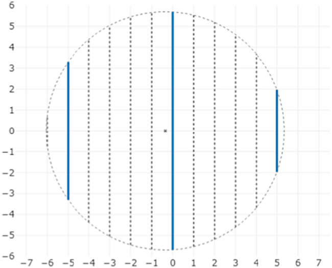
The disc of radius
$ {r} = 5.7 $
 , highlighting the chords formed by the lines spaced by
$ 1 $
 unit, and the lines spaced by
$ 5 $
 units. The behaviour of
${u}({x})$
 can be considered at either scale.

Acknowledgements
The author thanks the reviewer for their feedback. Calculations were implemented in R [4] using RStudio [3] and devtools [Reference Wickham, Hester, Chang and Bryan6]. Figures were created using plotly [Reference Sievert5].