1 Introduction
Let
 $\unicode[STIX]{x1D703}$
be an arithmetic function,
 $\unicode[STIX]{x1D703}:\mathbb{N}\rightarrow \mathbb{R}\cup \{\infty \}$
. We write
 ${\mathcal{B}}$
(or
 ${\mathcal{B}}_{\unicode[STIX]{x1D703}}$
) to denote the set of positive integers containing
 $n=1$
and all those
 $n\geqslant 2$
with prime factorization
 $n=p_{1}^{\unicode[STIX]{x1D6FC}_{1}}\cdots p_{k}^{\unicode[STIX]{x1D6FC}_{k}}$
,
 $p_{1}<p_{2}<\cdots <p_{k}$
, which satisfy
 $$\begin{eqnarray}p_{j+1}\leqslant \unicode[STIX]{x1D703}(p_{1}^{\unicode[STIX]{x1D6FC}_{1}}\cdots p_{j}^{\unicode[STIX]{x1D6FC}_{j}})\quad (0\leqslant j<k),\end{eqnarray}$$
where
 $p_{1}^{\unicode[STIX]{x1D6FC}_{1}}\cdots p_{j}^{\unicode[STIX]{x1D6FC}_{j}}$
is understood to be
 $1$
when
 $j=0$
. Let
 $B(x)$
(or
 $B_{\unicode[STIX]{x1D703}}(x)$
) be the number of positive integers
 $n\leqslant x$
in
 ${\mathcal{B}}$
. The following list shows some examples of
 $\unicode[STIX]{x1D703}$
and its corresponding set
 ${\mathcal{B}}$
.
-
∙ If
 $\unicode[STIX]{x1D703}(n)=2n$
, then
${\mathcal{B}}$
is the set of integers with
$2$
-dense divisors, i.e. integers
$n$
which have a divisor in every interval
$[y,2y]$
for
$1\leqslant y\leqslant n$
(see [Reference Saias4, Reference Tenenbaum5, Reference Weingartner8]).
-
∙ If
$\unicode[STIX]{x1D703}(n)=\unicode[STIX]{x1D70E}(n)+1$
, where
$\unicode[STIX]{x1D70E}(n)$
is the sum-of-divisors function, then
${\mathcal{B}}$
is the set of practical numbers, i.e. integers
$n$
such that every
$1\leqslant m\leqslant n$
can be written as a sum of distinct positive divisors of
$n$
(see [Reference Saias4, Reference Tenenbaum5, Reference Weingartner8] and the references therein). -
∙ If
$\unicode[STIX]{x1D703}(n)=n+1$
, then
${\mathcal{B}}$
is the set of even
$\unicode[STIX]{x1D711}$
-practical numbers, i.e. even integers
$n$
such that the polynomial
$X^{n}-1$
has a divisor in
$\mathbb{Z}[X]$
of every degree from
$1$
to
$n$
(see [Reference Pomerance, Thompson and Weingartner2, Reference Thompson6, Reference Thompson7]).


Building on earlier work by Tenenbaum [Reference Tenenbaum5] and Saias [Reference Saias4], we found [Reference Weingartner8, Theorem 1.2] that
 $$\begin{eqnarray}B(x)\sim \frac{c_{\unicode[STIX]{x1D703}}x}{\log x}\quad (x\rightarrow \infty )\end{eqnarray}$$
for some positive constant
 $c_{\unicode[STIX]{x1D703}}$
, provided
 $\unicode[STIX]{x1D703}(n)$
satisfies
 $$\begin{eqnarray}\max (2,n)\leqslant \unicode[STIX]{x1D703}(n)\ll \frac{n\log 2n}{(\log \log 3n)^{1+\unicode[STIX]{x1D700}}}\quad (n\geqslant 1)\end{eqnarray}$$
for some
 $\unicode[STIX]{x1D700}>0$
. This applies to each of the three examples listed above.
In this note, our goal is to investigate the set
 ${\mathcal{B}}$
in general, without any restrictions on
 $\unicode[STIX]{x1D703}$
. We will show that
 ${\mathcal{B}}$
always has a natural density (Theorem 1) and provide a criterion to determine whether this natural density is positive or zero (Theorem 2). We give estimates for
 $B(x)$
with explicit error terms, first without any assumptions on
 $\unicode[STIX]{x1D703}$
(Theorem 1), and then under certain conditions on the size of
 $\unicode[STIX]{x1D703}(n)$
(Corollary 1 and Theorem 3).
As an application, we consider the following set, related to the distribution of divisors. Let
 ${\mathcal{D}}$
be the set of positive integers containing
 $n=1$
and all those
 $n\geqslant 2$
whose divisors
 $1=d_{1}<d_{2}<\cdots <d_{\unicode[STIX]{x1D70F}(n)}=n$
satisfy
 $$\begin{eqnarray}d_{j+1}\leqslant \unicode[STIX]{x1D703}(d_{j})\quad (1\leqslant j<\unicode[STIX]{x1D70F}(n)).\end{eqnarray}$$
We write
 $D(x)$
for the number of positive integers
 $n\leqslant x$
in
 ${\mathcal{D}}$
. Theorem 4 shows that
 ${\mathcal{B}}={\mathcal{D}}$
provided
 $\unicode[STIX]{x1D703}(n)/n$
is non-decreasing, so that all results concerning
 $B(x)$
also apply to
 $D(x)$
under this assumption.
2 Statement of results
Let
 $P^{+}(n)$
(respectively
 $P^{-}(n)$
) denote the largest (respectively smallest) prime factor of
 $n\geqslant 2$
and put
 $P^{+}(1)=1$
,
 $P^{-}(1)=\infty$
.
Note that replacing
 $\unicode[STIX]{x1D703}(n)$
by
 $\max (\unicode[STIX]{x1D703}(n),P^{+}(n))$
in (1) leaves the set
 ${\mathcal{B}}$
unchanged, because of the assumption
 $p_{1}<p_{2}<\cdots <p_{k}$
. Moreover, if
 $\unicode[STIX]{x1D703}(1)<2$
, then
 ${\mathcal{B}}=\{1\}$
. Thus, we may assume from now on, without any loss of generality, that
 $$\begin{eqnarray}\unicode[STIX]{x1D703}:\mathbb{N}\rightarrow \mathbb{R}\cup \{\infty \},\qquad \unicode[STIX]{x1D703}(1)\geqslant 2,\qquad \unicode[STIX]{x1D703}(n)\geqslant P^{+}(n)\qquad (n\geqslant 2).\end{eqnarray}$$
Let
 $\unicode[STIX]{x1D712}(n)$
be the characteristic function of the set
 ${\mathcal{B}}$
. We shall see in Lemma 4 that the series
 $$\begin{eqnarray}L=\mathop{\sum }_{n\geqslant 1}\frac{\unicode[STIX]{x1D712}(n)}{n}\mathop{\prod }_{p\leqslant \unicode[STIX]{x1D703}(n)}\biggl(1-\frac{1}{p}\biggr)\end{eqnarray}$$
converges to a value
 $0\leqslant L\leqslant 1$
. Theorem 1 shows that, for every choice of
 $\unicode[STIX]{x1D703}$
, the set
 ${\mathcal{B}}$
has a natural density, which is given by
 $1-L$
.
Theorem 1. Let
 $\unicode[STIX]{x1D703}$
satisfy (3). We have
 $$\begin{eqnarray}B(x)=(1-L)x+o(x).\end{eqnarray}$$
More precisely,
 $$\begin{eqnarray}B(x)=(1-L)x+O\biggl(1+x\mathop{\sum }_{n\geqslant 1}\frac{\unicode[STIX]{x1D712}(n)}{n\log \unicode[STIX]{x1D703}(n)}\exp \biggl(-\frac{\max (0,\log (x/n))}{3\log \unicode[STIX]{x1D703}(n)}\biggr)\biggr).\end{eqnarray}$$
Theorem 2 provides a simple criterion to determine whether
 $L=1$
and
 $B(x)=o(x)$
, or
 $L<1$
and
 $B(x)\sim (1-L)x$
.
Theorem 2. Let
 $\unicode[STIX]{x1D703}$
satisfy (3).
-
(i) Assume that
$\unicode[STIX]{x1D703}(n)\leqslant f(n)$
, where
$n\log f(n)$
is increasing. If diverges, then
$$\begin{eqnarray}\mathop{\sum }_{n\geqslant 1}\frac{1}{n\log f(n)}\end{eqnarray}$$
$L=1$
and
$B(x)=o(x)$
.
-
(ii) Assume that
$\unicode[STIX]{x1D703}(n)\geqslant f(n)\geqslant 2$
,
$f(n)\gg P^{+}(n)$
, and that for every
$t\geqslant 1$
there exists an
$r\in \mathbb{N}$
such that
$f(2^{r}n)\geqslant tf(n)$
for all
$n\geqslant 1$
. If converges, then
$$\begin{eqnarray}\mathop{\sum }_{n\geqslant 1}\frac{1}{n\log f(n)}\end{eqnarray}$$
$L<1$
and
$B(x)\sim (1-L)x$
.
-
(iii)
$B(x)\sim x\Leftrightarrow L=0\Leftrightarrow \unicode[STIX]{x1D703}(n)=\infty$
for all
$n\geqslant 1\Leftrightarrow B(x)=[x]$
.


Note that the three examples of
 $\unicode[STIX]{x1D703}$
listed in the introduction satisfy
 $L=1$
and
 $B(x)=o(x)$
. For an instance where
 $L<1$
, consider
 $\unicode[STIX]{x1D703}(n)=2^{n}$
, for which
 $L=0.7734\ldots$
by numerical computation. (For
 $n\geqslant 30$
, we used estimates for the Euler product with effective error bounds due to Rosser and Schoenfeld [Reference Rosser and Schoenfeld3, Theorem 7].) Hence, (4) implies that
 $B(x)=cx(1+o(1))$
with
 $c=1-L=0.2265\ldots ,$
while (5) shows that we have
 $B(x)=cx(1+O(1/\text{log}\,x))$
when
 $\unicode[STIX]{x1D703}(n)=2^{n}$
.
Corollary 1 generalizes this example to
 $\log \unicode[STIX]{x1D703}(n)\asymp n^{a}$
, where
 $a$
is a positive constant. We also consider the case
 $\log \unicode[STIX]{x1D703}(n)\asymp (\log 2n)^{a}$
, where
 $a>1$
is constant. (The notation
 $f(n)\asymp g(n)$
means that
 $f(n)\ll g(n)$
(i.e.
 $f(n)=O(g(n))$
) and
 $g(n)\ll f(n)$
.)
Corollary 1. Let
 $\unicode[STIX]{x1D703}$
satisfy (3).
-
(i) If
$\log \unicode[STIX]{x1D703}(n)\asymp n^{a}$
for some constant
$a>0$
, then
$0<L<1$
and
$$\begin{eqnarray}B(x)=(1-L)x\biggl(1+O\biggl(\frac{1}{\log x}\biggr)\biggr).\end{eqnarray}$$
-
(ii) If
$\log \unicode[STIX]{x1D703}(n)\asymp (\log 2n)^{a}$
for some constant
$a>1$
, then
$0<L<1$
and
$$\begin{eqnarray}B(x)=(1-L)x\biggl(1+O\biggl(\frac{1}{(\log x)^{1-1/a}}\biggr)\biggr).\end{eqnarray}$$


The error terms in Corollary 1 are easily derived from (5), using the trivial bound
 $\unicode[STIX]{x1D712}(n)\leqslant 1$
. The claim that
 $0<L<1$
follows directly from Theorem 2, with (i)
 $f(n)=\max (2,\exp (cn^{a}))$
and (ii)
 $f(n)=\max (2,\exp (c(\log 2n)^{a}))$
, where
 $c>0$
is a suitable constant. Other examples of
 $\unicode[STIX]{x1D703}$
, for which
 $L<1$
, can be dealt with similarly.
When
 $B(x)=o(x)$
, we need a different strategy for obtaining an asymptotic formula for
 $B(x)$
, since the estimate (5) provides only an upper bound for
 $B(x)$
whenever
 $L=1$
. We will focus on the case
 $\unicode[STIX]{x1D703}(n)\asymp n^{a}$
, where
 $a\geqslant 1$
is constant. Theorem 2 shows that
 $L=1$
and
 $B(x)=o(x)$
. Theorem 3 generalizes [Reference Weingartner8, Theorem 1.2], where the case
 $a=1$
is established with
 $\unicode[STIX]{x1D706}_{1}=1$
.
Theorem 3. Let
 $\unicode[STIX]{x1D703}$
satisfy (3) and assume that
 $\unicode[STIX]{x1D703}(n)\asymp n^{a}$
for some constant
 $a\geqslant 1$
. Then there are constants
 $c_{\unicode[STIX]{x1D703}}>0$
and
 $\unicode[STIX]{x1D706}_{a}\in (0,1]$
such that
 $$\begin{eqnarray}B(x)=\frac{c_{\unicode[STIX]{x1D703}}x}{(\log x)^{\unicode[STIX]{x1D706}_{a}}}\biggl(1+O\biggl(\frac{1}{\log x}\biggr)\biggr).\end{eqnarray}$$
Here
 $s=-\unicode[STIX]{x1D706}_{a}$
is the unique solution in the interval
 $[-1,0)$
of the equation
 $$\begin{eqnarray}0=s+\frac{\text{e}^{-\unicode[STIX]{x1D6FE}}}{a(a+1)^{s}}+s\int _{1}^{\infty }(\unicode[STIX]{x1D714}(t)-\text{e}^{-\unicode[STIX]{x1D6FE}})\frac{dt}{(at+1)^{s+1}},\end{eqnarray}$$
where
 $\unicode[STIX]{x1D714}(t)$
denotes Buchstab’s function and
 $\unicode[STIX]{x1D6FE}$
is Euler’s constant. For
 $a\geqslant 1$
,
 $$\begin{eqnarray}\unicode[STIX]{x1D706}_{a}>\frac{\text{e}^{-\unicode[STIX]{x1D6FE}}}{a}\biggl(1+\frac{\text{e}^{-\unicode[STIX]{x1D6FE}}\log (a+1)}{a}-\frac{0.16}{a}\biggr)\end{eqnarray}$$
and
 $$\begin{eqnarray}\unicode[STIX]{x1D706}_{a}<\frac{\text{e}^{-\unicode[STIX]{x1D6FE}}}{a}\biggl(1+\frac{\text{e}^{-\unicode[STIX]{x1D6FE}}\log (a+1)}{a}+\frac{\log ^{2}(a+1)}{a^{2}}\biggr).\end{eqnarray}$$
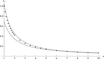
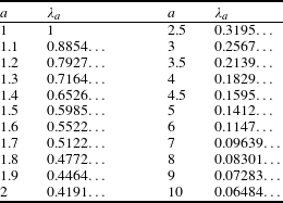
Figure 1 and Table 1 show several values of
 $\unicode[STIX]{x1D706}_{a}$
, obtained by solving equation (7) numerically.
As in [Reference Weingartner8, Theorem 1.2] with
 $a=1$
, one can consider a less restrictive condition on
 $\unicode[STIX]{x1D703}$
, such as
 $n^{a}(\log n)^{-b}\ll \unicode[STIX]{x1D703}(n)\ll n^{a}(\log n)^{b}$
, where
 $0\leqslant b<1$
, and establish the estimate (6) with the relative error term
 $O(1/\text{log}\,x)$
replaced by
 $O(1/(\log x)^{1-b})$
. However, we will not pursue this here.


Truncated values of
 $\unicode[STIX]{x1D706}_{a}$
.

We now turn to the distribution of divisors. Let
 ${\mathcal{D}}$
be the set defined in (2). When
 $\unicode[STIX]{x1D703}(n)=tn$
, where
 $t$
is constant, Tenenbaum [Reference Tenenbaum5, Lemma 2.2] showed that
 ${\mathcal{D}}={\mathcal{B}}$
. We want to generalize this result as much as possible. The example
 $\unicode[STIX]{x1D703}(n)=n+1$
, for which
 ${\mathcal{D}}=\{1,2\}$
while
 ${\mathcal{B}}$
is infinite, illustrates that some condition on
 $\unicode[STIX]{x1D703}$
is required to ensure equality of these two sets. The condition we need is
 $$\begin{eqnarray}\unicode[STIX]{x1D703}(n)\leqslant \unicode[STIX]{x1D703}(n+1),\qquad m\unicode[STIX]{x1D703}(n)\leqslant \unicode[STIX]{x1D703}(mn)\quad (n,m\geqslant 1,\gcd (n,m)=1).\end{eqnarray}$$
Note that (10) is satisfied if
 $\unicode[STIX]{x1D703}(n)/n$
is non-decreasing.
Theorem 4. Let
 $\unicode[STIX]{x1D703}$
satisfy (3).
-
(i) We have
${\mathcal{D}}\subseteq {\mathcal{B}}$
and hence
$D(x)\leqslant B(x)$
. -
(ii) If
$\unicode[STIX]{x1D703}$
satisfies (10), then
${\mathcal{D}}={\mathcal{B}}$
and hence
$D(x)=B(x)$
.


As an example, consider
 $\unicode[STIX]{x1D703}(n)=n^{2}+1$
. Theorems 3 and 4 show that the number of integers
 $n\leqslant x$
whose divisors
 $1=d_{1}<d_{2}<\cdots <d_{\unicode[STIX]{x1D70F}(n)}=n$
satisfy
 $d_{j+1}\leqslant d_{j}^{2}+1$
for
 $1\leqslant j<\unicode[STIX]{x1D70F}(n)$
is given by
 $$\begin{eqnarray}D(x)=\frac{cx}{(\log x)^{\unicode[STIX]{x1D706}_{2}}}\biggl(1+O\biggl(\frac{1}{\log x}\biggr)\biggr),\end{eqnarray}$$
where
 $c$
is a positive constant and
 $\unicode[STIX]{x1D706}_{2}=0.4191\ldots \,$
.
With
 $\unicode[STIX]{x1D703}(n)=2^{n}$
, Corollary 1 and Theorem 4 show that the number of integers
 $n\leqslant x$
whose divisors
 $1=d_{1}<d_{2}<\cdots <d_{\unicode[STIX]{x1D70F}(n)}=n$
satisfy
 $d_{j+1}\leqslant 2^{d_{j}}$
for
 $1\leqslant j<\unicode[STIX]{x1D70F}(n)$
is given by
 $$\begin{eqnarray}D(x)=(1-L)x\biggl(1+O\biggl(\frac{1}{\log x}\biggr)\biggr),\end{eqnarray}$$
where
 $1-L=0.2265\ldots \,$
.
The proof of Theorem 1 is based on the functional equation in Lemma 3 and an estimate for the number of integers without small prime factors in Lemma 2. Theorem 2 is established with the help of Theorem 1. The proof of Theorem 3, which requires the most amount of work, is modeled after [Reference Weingartner8, Theorem 1.2], with the added difficulty that the poles of the Laplace transform (i.e. the solutions of equation (7)) now depend on the parameter
 $a$
(see Lemma 9). The proof of Theorem 4 generalizes that of Tenenbaum [Reference Tenenbaum5, Lemma 2.2].
3 Preliminaries
Let
 $$\begin{eqnarray}\unicode[STIX]{x1D6F7}(x,y)=\#\{1\leqslant n\leqslant x:P^{-}(n)>y\}\end{eqnarray}$$
and define
 $\unicode[STIX]{x1D6F7}(x,\infty )=1$
for
 $x\geqslant 1$
. For
 $u\geqslant 1$
, Buchstab’s function
 $\unicode[STIX]{x1D714}(u)$
is defined as the unique continuous solution to the equation
 $$\begin{eqnarray}(u\unicode[STIX]{x1D714}(u))^{\prime }=\unicode[STIX]{x1D714}(u-1)\quad (u>2)\end{eqnarray}$$
with initial condition
 $u\unicode[STIX]{x1D714}(u)=1$
for
 $1\leqslant u\leqslant 2$
. Let
 $\unicode[STIX]{x1D714}(u)=0$
for
 $u<1$
and define
 $\unicode[STIX]{x1D714}$
at 1 and
 $\unicode[STIX]{x1D714}^{\prime }$
at 1 and 2 by right-continuity. Let
 $\unicode[STIX]{x1D6E4}(u)$
denote the usual gamma function.
The calculation of the values of
 $\unicode[STIX]{x1D706}_{a}$
in Table 1 and the approximation of several integrals in the proof of Lemma 9 require estimates for integrals involving
 $\unicode[STIX]{x1D714}(t)-\text{e}^{-\unicode[STIX]{x1D6FE}}$
. For that purpose, we used exact formulas for
 $\unicode[STIX]{x1D714}(t)$
for
 $0\leqslant t\leqslant 5$
, derived with the help of Mathematica. To estimate the contribution from
 $t>5$
, we used a table of zeros and relative extrema of
 $\unicode[STIX]{x1D714}(t)-\text{e}^{-\unicode[STIX]{x1D6FE}}$
on the interval
 $[5,10.3355]$
due to Cheer and Goldston [Reference Cheer and Goldston1], and the estimate (ii) from Lemma 1 for
 $t\geqslant 10.3355$
.
Lemma 1. We have:
-
(i)
$|\unicode[STIX]{x1D714}^{\prime }(u)|\leqslant 1/\unicode[STIX]{x1D6E4}(u+1)\quad (u\geqslant 0)$
; -
(ii)
$|\unicode[STIX]{x1D714}(u)-\text{e}^{-\unicode[STIX]{x1D6FE}}|\leqslant 1/\unicode[STIX]{x1D6E4}(u+1)\quad (u\geqslant 0)$
.


Proof. See [Reference Weingartner8, Lemma 2.1].◻
Lemma 2. Let
 $u=\log x/\text{log}\,y$
.
-
(i) For
$x\geqslant 1$
,
$y\geqslant 2$
, we have
$$\begin{eqnarray}\unicode[STIX]{x1D6F7}(x,y)=\text{e}^{\unicode[STIX]{x1D6FE}}x\unicode[STIX]{x1D714}(u)\mathop{\prod }_{p\leqslant y}\biggl(1-\frac{1}{p}\biggr)+O\biggl(\frac{y}{\log y}+\frac{x\text{e}^{-u/3}}{(\log y)^{2}}\biggr).\end{eqnarray}$$
-
(ii) For
$x\geqslant y\geqslant 2$
, we have
$$\begin{eqnarray}\unicode[STIX]{x1D6F7}(x,y)=x\mathop{\prod }_{p\leqslant y}\biggl(1-\frac{1}{p}\biggr)+O\biggl(\frac{x\text{e}^{-u/3}}{\log y}\biggr).\end{eqnarray}$$


Proof. (i) See [Reference Weingartner8, Lemma 2.2]. Part (ii) follows from (i) and Lemma 1.◻
Lemma 3. Let
 $\unicode[STIX]{x1D703}$
satisfy (3). For
 $x\geqslant 0$
, we have
 $$\begin{eqnarray}[x]=\mathop{\sum }_{n\leqslant x}\unicode[STIX]{x1D712}(n)\,\unicode[STIX]{x1D6F7}(x/n,\unicode[STIX]{x1D703}(n)).\end{eqnarray}$$
Proof. In [Reference Weingartner8, Lemma 2.3], we proved this result assuming that
 $\unicode[STIX]{x1D703}(n)<\infty$
. The inclusion of
 $\infty$
in the possible values of
 $\unicode[STIX]{x1D703}$
has no effect on the proof. The basic idea is that every integer
 $1\leqslant m\leqslant x$
factors uniquely as
 $m=nr$
, where
 $n\in {\mathcal{B}}$
and
 $r$
is counted in
 $\unicode[STIX]{x1D6F7}(x/n,\unicode[STIX]{x1D703}(n))$
.◻
Lemma 4. Let
 $\unicode[STIX]{x1D703}$
satisfy (3). The series
 $$\begin{eqnarray}L=\mathop{\sum }_{n\geqslant 1}\frac{\unicode[STIX]{x1D712}(n)}{n}\mathop{\prod }_{p\leqslant \unicode[STIX]{x1D703}(n)}\biggl(1-\frac{1}{p}\biggr)\end{eqnarray}$$
converges and
 $0\leqslant L\leqslant 1$
.
Proof. Lemma 2(ii) implies that
 $\lim _{x\rightarrow \infty }\unicode[STIX]{x1D6F7}(x,y)/x=\prod _{p\leqslant y}(1-1/p)$
. From Lemma 3, we have
 $$\begin{eqnarray}\mathop{\sum }_{1\leqslant n\leqslant N}\frac{\unicode[STIX]{x1D712}(n)}{n}\mathop{\prod }_{p\leqslant \unicode[STIX]{x1D703}(n)}\biggl(1-\frac{1}{p}\biggr)\leqslant 1\end{eqnarray}$$
for every
 $N\geqslant 1$
. The result now follows since the terms of the series are
 ${\geqslant}0$
.◻
4 Proof of Theorems 1 and 2
Proof of Theorem 1.
Since
 $\unicode[STIX]{x1D6F7}(x/n,\unicode[STIX]{x1D703}(n))=1$
when
 $n\leqslant x<n\unicode[STIX]{x1D703}(n)$
, Lemma 3 yields
 $$\begin{eqnarray}\displaystyle [x] & = & \displaystyle B(x)+\mathop{\sum }_{n\leqslant x}\unicode[STIX]{x1D712}(n)\,(\unicode[STIX]{x1D6F7}(x/n,\unicode[STIX]{x1D703}(n))-1)\nonumber\\ \displaystyle & = & \displaystyle B(x)+\mathop{\sum }_{n\unicode[STIX]{x1D703}(n)\leqslant x}\unicode[STIX]{x1D712}(n)\,(\unicode[STIX]{x1D6F7}(x/n,\unicode[STIX]{x1D703}(n))-1)\nonumber\\ \displaystyle & = & \displaystyle B(x)+x\mathop{\sum }_{n\unicode[STIX]{x1D703}(n)\leqslant x}\frac{\unicode[STIX]{x1D712}(n)}{n}\mathop{\prod }_{p\leqslant \unicode[STIX]{x1D703}(n)}\biggl(1-\frac{1}{p}\biggr)+O(E_{1}(x)),\nonumber\end{eqnarray}$$
where
 $$\begin{eqnarray}E_{1}(x)=x\mathop{\sum }_{n\unicode[STIX]{x1D703}(n)\leqslant x}\frac{\unicode[STIX]{x1D712}(n)}{n\log \unicode[STIX]{x1D703}(n)}\exp \biggl(-\frac{\log (x/n)}{3\log \unicode[STIX]{x1D703}(n)}\biggr),\end{eqnarray}$$
by Lemma 2(ii). Thus,
 $$\begin{eqnarray}[x]=B(x)+Lx+O(E_{1}(x)+E_{2}(x)),\end{eqnarray}$$
where
 $$\begin{eqnarray}E_{2}(x)=x\mathop{\sum }_{n\unicode[STIX]{x1D703}(n)>x}\frac{\unicode[STIX]{x1D712}(n)}{n\log \unicode[STIX]{x1D703}(n)}.\end{eqnarray}$$
This completes the proof of (5). The estimate (4) follows, since
 $E_{1}(x)+E_{2}(x)=o(x)$
, by Lemma 4.◻
Proof of Theorem 2.
(i) Assume that
 $L<1$
, so that
 $B(n)\geqslant cn$
for some
 $c>0$
and all
 $n\geqslant 1$
. Let
 $g(n)=\log f(n)$
and assume that
 $ng(n)$
is increasing. Partial summation applied twice yields
 $$\begin{eqnarray}\displaystyle \mathop{\sum }_{n\leqslant N}\frac{\unicode[STIX]{x1D712}(n)}{ng(n)} & = & \displaystyle \frac{B(N)}{Ng(N)}+\mathop{\sum }_{n\leqslant N-1}B(n)\biggl(\frac{1}{ng(n)}-\frac{1}{(n+1)g(n+1)}\biggr)\nonumber\\ \displaystyle & {\geqslant} & \displaystyle \frac{cN}{Ng(N)}+\mathop{\sum }_{n\leqslant N-1}cn\biggl(\frac{1}{ng(n)}-\frac{1}{(n+1)g(n+1)}\biggr)\nonumber\\ \displaystyle & = & \displaystyle \mathop{\sum }_{n\leqslant N}\frac{c}{ng(n)},\nonumber\end{eqnarray}$$
which grows unbounded as
 $N$
increases. But this is impossible, since
 $$\begin{eqnarray}\mathop{\sum }_{n\leqslant N}\frac{\unicode[STIX]{x1D712}(n)}{ng(n)}\leqslant \mathop{\sum }_{n\leqslant N}\frac{\unicode[STIX]{x1D712}(n)}{n\log \unicode[STIX]{x1D703}(n)}\ll \mathop{\sum }_{n\leqslant N}\frac{\unicode[STIX]{x1D712}(n)}{n}\mathop{\prod }_{p\leqslant \unicode[STIX]{x1D703}(n)}\biggl(1-\frac{1}{p}\biggr)\leqslant L\leqslant 1,\end{eqnarray}$$
by Lemma 4. Thus,
 $L=1$
and
 $B(x)=o(x)$
.
(ii) Assume that
 $\unicode[STIX]{x1D703}(n)\geqslant f(n)\geqslant 2$
, where
 $f(n)\gg P^{+}(n)$
, and that
 $$\begin{eqnarray}\mathop{\sum }_{n\geqslant 1}\frac{1}{n\log f(n)}\end{eqnarray}$$
converges. Then there exists a
 $t\geqslant 1$
such that
 $tf(n)\geqslant P^{+}(n)$
and
 $$\begin{eqnarray}L_{tf}\leqslant \mathop{\sum }_{n\geqslant 1}\frac{1}{n}\mathop{\prod }_{p\leqslant tf(n)}\biggl(1-\frac{1}{p}\biggr)<1.\end{eqnarray}$$
Theorem 1 implies that
 $B_{tf}(x)\gg x$
. According to the hypothesis, there is an
 $r\in \mathbb{N}$
such that
 $f(2^{r}n)\geqslant tf(n)$
for all
 $n\geqslant 1$
. Thus, if
 $n$
is counted in
 $B_{tf}(x/2^{r})$
, then
 $2^{r}n$
is counted in
 $B_{f}(x)$
. This yields
 $$\begin{eqnarray}B_{\unicode[STIX]{x1D703}}(x)\geqslant B_{f}(x)\geqslant B_{tf}(x/2^{r})\gg _{r}x.\end{eqnarray}$$
Part (iii) is an immediate consequence of Theorem 1.◻
5 Proof of Theorem 3
Throughout this section, we assume that
 $\unicode[STIX]{x1D703}$
satisfies (3) and that
 $$\begin{eqnarray}B(x)\ll \frac{x}{(\log x)^{\unicode[STIX]{x1D708}}}\quad (x\geqslant 2)\end{eqnarray}$$
for some suitable
 $\unicode[STIX]{x1D708}\in [0,1]$
, to be determined later. Clearly,
 $\unicode[STIX]{x1D708}=0$
is admissible. All constants implied by
 $\ll$
and the big O notation may depend on
 $\unicode[STIX]{x1D703}$
, and therefore on
 $a$
, but are otherwise absolute. Lemmas 5 through 8 correspond to Lemmas 5.3 through 5.7 of [Reference Weingartner8]. The main difference is the assumption on the size of
 $B(x)$
for the purpose of estimating the error terms, for which we use (11) here.
Lemma 5. For
 $x\geqslant e$
, we have
 $$\begin{eqnarray}\displaystyle B(x)=x-x\!\mathop{\sum }_{n\unicode[STIX]{x1D703}(n)\leqslant x}\!\frac{\unicode[STIX]{x1D712}(n)}{n}\,\text{e}^{\unicode[STIX]{x1D6FE}}\unicode[STIX]{x1D714}\biggl(\frac{\log x/n}{\log \unicode[STIX]{x1D703}(n)}\biggr)\!\!\mathop{\prod }_{p\leqslant \unicode[STIX]{x1D703}(n)}\biggl(1-\frac{1}{p}\biggr)+O\biggl(\frac{x}{(\log x)^{1+\unicode[STIX]{x1D708}}}\biggr). & & \displaystyle \nonumber\end{eqnarray}$$
Proof. As in the proof of Theorem 1, we have
 $$\begin{eqnarray}B(x)=[x]-\mathop{\sum }_{n\unicode[STIX]{x1D703}(n)\leqslant x}\unicode[STIX]{x1D712}(n)\,(\unicode[STIX]{x1D6F7}(x/n,\unicode[STIX]{x1D703}(n))-1).\end{eqnarray}$$
We apply Lemma 2(i) to estimate each occurrence of
 $\unicode[STIX]{x1D6F7}(x/n,\unicode[STIX]{x1D703}(n))$
in (12). The contribution from the error term
 $O(y/\text{log}\,y)$
is
 $$\begin{eqnarray}\displaystyle & \ll & \displaystyle \mathop{\sum }_{n\unicode[STIX]{x1D703}(n)\leqslant x}\unicode[STIX]{x1D712}(n)\frac{\unicode[STIX]{x1D703}(n)}{\log \unicode[STIX]{x1D703}(n)}\ll \mathop{\sum }_{n^{1+a}\ll x}\unicode[STIX]{x1D712}(n)\frac{n^{a}}{\log 2n}\nonumber\\ \displaystyle & \ll & \displaystyle \frac{x^{a/(1+a)}}{\log x}\mathop{\sum }_{n\ll x^{1/(1+a)}}\unicode[STIX]{x1D712}(n)\ll \frac{x}{(\log x)^{\unicode[STIX]{x1D708}+1}},\nonumber\end{eqnarray}$$
by (11). For the contribution from the error term
 $O(x\text{e}^{-u/3}/(\log y)^{2})$
, we split up the range of summation by powers of
 $2$
and use (11) to get
 $$\begin{eqnarray}\displaystyle & \ll & \displaystyle \mathop{\sum }_{n\unicode[STIX]{x1D703}(n)\leqslant x}\unicode[STIX]{x1D712}(n)\frac{x}{n(\log \unicode[STIX]{x1D703}(n))^{2}}\exp \biggl(-\frac{\log x/n}{3\log \unicode[STIX]{x1D703}(n)}\biggr)\nonumber\\ \displaystyle & \ll & \displaystyle \mathop{\sum }_{n\ll x^{1/(1+a)}}\frac{x}{n(\log 2n)^{2+\unicode[STIX]{x1D708}}}\exp \biggl(-\frac{\log 2x}{A\log 2n}\biggr)\ll \frac{x}{(\log x)^{1+\unicode[STIX]{x1D708}}},\nonumber\end{eqnarray}$$
where
 $A$
is some suitable positive constant.◻
Lemma 6. For
 $x\geqslant e$
, we have
 $$\begin{eqnarray}B(x)=x\mathop{\sum }_{n\geqslant 1}\frac{\unicode[STIX]{x1D712}(n)}{n\log \unicode[STIX]{x1D703}(n)}\biggl(\text{e}^{-\unicode[STIX]{x1D6FE}}-\unicode[STIX]{x1D714}\biggl(\frac{\log x/n}{\log \unicode[STIX]{x1D703}(n)}\biggr)\biggr)+O\biggl(\frac{x}{(\log x)^{1+\unicode[STIX]{x1D708}}}\biggr).\end{eqnarray}$$
Proof. We have
 $L=1$
by Theorem 2. Since
 $\unicode[STIX]{x1D714}(u)=0$
for
 $u<1$
, Lemma 5 shows that
 $$\begin{eqnarray}\displaystyle B(x)=x\mathop{\sum }_{n\geqslant 1}\frac{\unicode[STIX]{x1D712}(n)}{n}\!\mathop{\prod }_{p\leqslant \unicode[STIX]{x1D703}(n)}\biggl(1-\frac{1}{p}\biggr)\biggl(1-\text{e}^{\unicode[STIX]{x1D6FE}}\unicode[STIX]{x1D714}\biggl(\frac{\log x/n}{\log \unicode[STIX]{x1D703}(n)}\biggr)\biggr)+O\biggl(\frac{x}{(\log x)^{1+\unicode[STIX]{x1D708}}}\biggr). & & \displaystyle \nonumber\end{eqnarray}$$
The contribution from
 $n$
with
 $\log n\leqslant \sqrt{\log x}$
is
 $\ll x\exp (-\sqrt{\log x})$
. For those
 $n$
for which
 $\log n>\sqrt{\log x}$
, we use the estimate
 $$\begin{eqnarray}\mathop{\prod }_{p\leqslant \unicode[STIX]{x1D703}(n)}\biggl(1-\frac{1}{p}\biggr)=\frac{\text{e}^{-\unicode[STIX]{x1D6FE}}}{\log \unicode[STIX]{x1D703}(n)}\biggl(1+O\biggl(\frac{1}{(\log n)^{4}}\biggr)\biggr).\end{eqnarray}$$
The contribution from the error term is
 $$\begin{eqnarray}\ll x\mathop{\sum }_{\log n>\sqrt{\log x}}\frac{1}{n(\log n)^{5}}\ll \frac{x}{(\log x)^{2}}\ll \frac{x}{(\log x)^{1+\unicode[STIX]{x1D708}}}.\square\end{eqnarray}$$
Lemma 7. For
 $x\geqslant e$
, we have
 $$\begin{eqnarray}B(x)=x\mathop{\sum }_{n\geqslant 2}\frac{\unicode[STIX]{x1D712}(n)}{an\log n}\biggl(\text{e}^{-\unicode[STIX]{x1D6FE}}-\unicode[STIX]{x1D714}\biggl(\frac{\log x/n}{a\log n}\biggr)\biggr)+O\biggl(\frac{x}{(\log x)^{1+\unicode[STIX]{x1D708}}}\biggr).\end{eqnarray}$$
Proof. Since
 $\unicode[STIX]{x1D703}(n)\asymp n^{a}$
, we have
 $\log \unicode[STIX]{x1D703}(n)=a\log n+O(1)$
. Inserting this estimate for each instance of
 $\log \unicode[STIX]{x1D703}(n)$
in Lemma 6 yields the desired result. For more details of the calculations, see [Reference Weingartner8, Lemma 5.6], where the case
 $a=1$
is treated.◻
Lemma 8. For
 $x\geqslant e$
, we have
 $$\begin{eqnarray}B(x)=x\int _{\text{e}}^{\infty }\frac{B(y)}{ay^{2}\log y}\biggl(\text{e}^{-\unicode[STIX]{x1D6FE}}-\unicode[STIX]{x1D714}\biggl(\frac{\log x/y}{a\log y}\biggr)\biggr)\,dy+O\biggl(\frac{x}{(\log x)^{1+\unicode[STIX]{x1D708}}}\biggr).\end{eqnarray}$$
Proof. This follows from applying partial summation to the sum in Lemma 7. ◻
From Lemma 8, we have, for
 $x\geqslant e$
,
 $$\begin{eqnarray}B(x)=x\,\unicode[STIX]{x1D6FC}-x\int _{\text{e}}^{\infty }\frac{B(y)}{ay^{2}\log y}\,\unicode[STIX]{x1D714}\biggl(\frac{\log x/y}{a\log y}\biggr)\,dy+O\biggl(\frac{x}{(\log x)^{1+\unicode[STIX]{x1D708}}}\biggr),\end{eqnarray}$$
where
 $$\begin{eqnarray}\unicode[STIX]{x1D6FC}:=\text{e}^{-\unicode[STIX]{x1D6FE}}\int _{\text{e}}^{\infty }\frac{B(y)}{ay^{2}\log y}\,dy.\end{eqnarray}$$
For
 $x\geqslant e$
, let
 $z\geqslant 0$
be given by
 $$\begin{eqnarray}z=\log \log (x)\end{eqnarray}$$
and let
 $$\begin{eqnarray}G_{\unicode[STIX]{x1D703}}(z):=\frac{B(\exp (\text{e}^{z}))}{\exp (\text{e}^{z})}=\frac{B(x)}{x}.\end{eqnarray}$$
Dividing (13) by
 $x$
and changing variables in the integral via
 $u=\log \log y$
, we get, for
 $z\geqslant 0$
,
 $$\begin{eqnarray}\displaystyle G_{\unicode[STIX]{x1D703}}(z) & = & \displaystyle \unicode[STIX]{x1D6FC}-\frac{1}{a}\int _{0}^{z}G_{\unicode[STIX]{x1D703}}(u)\,\unicode[STIX]{x1D714}((\text{e}^{z-u}-1)/a)\,du+E_{\unicode[STIX]{x1D703}}(z)\nonumber\\ \displaystyle & = & \displaystyle \unicode[STIX]{x1D6FC}-\frac{1}{a}\int _{0}^{z}G_{\unicode[STIX]{x1D703}}(u)\,\unicode[STIX]{x1D6FA}_{a}(z-u)\,du+E_{\unicode[STIX]{x1D703}}(z),\end{eqnarray}$$
where
 $$\begin{eqnarray}E_{\unicode[STIX]{x1D703}}(z)\ll \text{e}^{-(1+\unicode[STIX]{x1D708})z}\end{eqnarray}$$
and
 $$\begin{eqnarray}\unicode[STIX]{x1D6FA}_{a}(u):=\unicode[STIX]{x1D714}((\text{e}^{u}-1)/a).\end{eqnarray}$$
Equation (14) leads to the equation of Laplace transforms
 $$\begin{eqnarray}\widehat{G}_{\unicode[STIX]{x1D703}}(s)=\frac{\unicode[STIX]{x1D6FC}}{s}-\frac{1}{a}\widehat{G}_{\unicode[STIX]{x1D703}}(s)\,\widehat{\unicode[STIX]{x1D6FA}}_{a}(s)+\widehat{E}_{\unicode[STIX]{x1D703}}(s)\quad (\text{Re}(s)>0),\end{eqnarray}$$
which we solve for
 $\widehat{G}_{\unicode[STIX]{x1D703}}(s)$
to get
 $$\begin{eqnarray}\widehat{G}_{\unicode[STIX]{x1D703}}(s)=\frac{\unicode[STIX]{x1D6FC}}{s(1+(1/a)\widehat{\unicode[STIX]{x1D6FA}}_{a}(s))}+\frac{\widehat{E}_{\unicode[STIX]{x1D703}}(s)}{1+(1/a)\widehat{\unicode[STIX]{x1D6FA}}_{a}(s)}\quad (\text{Re}(s)>0).\end{eqnarray}$$
Let
 $F_{a}(z)$
be given by
 $$\begin{eqnarray}F_{a}(z)=1-\frac{1}{a}\int _{0}^{z}F_{a}(u)\,\unicode[STIX]{x1D6FA}_{a}(z-u)\,du.\end{eqnarray}$$
Equation (16) is an error-free, rescaled version of equation (14), which depends on
 $a$
, but does not involve
 $\unicode[STIX]{x1D703}$
. Note that the upper limit of the integral could be replaced by
 $z-\log (a+1)$
, since
 $\unicode[STIX]{x1D714}(t)=0$
for
 $t<1$
. Thus,
 $F_{a}(z)=1$
for
 $0\leqslant z\leqslant \log (a+1)$
and, for
 $z>\log (a+1)$
,
 $F_{a}(z)$
is determined by the values of
 $F_{a}(u)$
for
 $u\in [0,z-\log (a+1)]$
. Hence, (16) defines the continuous function
 $F_{a}(z)$
for
 $z\geqslant 0$
. As with
 $G_{\unicode[STIX]{x1D703}}(z)$
, we find that the Laplace transform of
 $F_{a}(z)$
is given by
 $$\begin{eqnarray}\widehat{F}_{a}(s)=\frac{1}{s(1+(1/a)\widehat{\unicode[STIX]{x1D6FA}}_{a}(s))}\quad (\text{Re}(s)>0)\end{eqnarray}$$
and, therefore,
 $$\begin{eqnarray}\widehat{G}_{\unicode[STIX]{x1D703}}(s)=\unicode[STIX]{x1D6FC}\widehat{F}_{a}(s)+s\widehat{F}_{a}(s)\widehat{E}_{\unicode[STIX]{x1D703}}(s).\end{eqnarray}$$
The Laplace transform of
 $\unicode[STIX]{x1D6FA}_{a}(u)$
, defined for
 $\text{Re}(s)>0$
, is given by
 $$\begin{eqnarray}\displaystyle \widehat{\unicode[STIX]{x1D6FA}}_{a}(s) & = & \displaystyle \int _{0}^{\infty }\unicode[STIX]{x1D714}((\text{e}^{u}-1)/a)\text{e}^{-us}\,du=a\int _{0}^{\infty }\unicode[STIX]{x1D714}(t)\frac{dt}{(at+1)^{s+1}}\nonumber\\ \displaystyle & = & \displaystyle \frac{\text{e}^{-\unicode[STIX]{x1D6FE}}}{s(a+1)^{s}}+a\int _{1}^{\infty }(\unicode[STIX]{x1D714}(t)-\text{e}^{-\unicode[STIX]{x1D6FE}})\frac{dt}{(at+1)^{s+1}}.\nonumber\end{eqnarray}$$
The last equation extends
 $\widehat{\unicode[STIX]{x1D6FA}}_{a}(s)$
to a meromorphic function on
 $\mathbb{C}$
with a simple pole at
 $s=0$
. We will need to investigate the location of zeros of the entire function
 $g_{a}(s)$
, defined by
 $$\begin{eqnarray}\displaystyle g_{a}(s) & = & \displaystyle 1/\widehat{F}_{a}(s)=s\biggl(1+\frac{1}{a}\widehat{\unicode[STIX]{x1D6FA}}_{a}(s)\biggr)\nonumber\\ \displaystyle & = & \displaystyle s+\frac{\text{e}^{-\unicode[STIX]{x1D6FE}}}{a(a+1)^{s}}+s\int _{1}^{\infty }(\unicode[STIX]{x1D714}(t)-\text{e}^{-\unicode[STIX]{x1D6FE}})\frac{dt}{(at+1)^{s+1}}.\nonumber\end{eqnarray}$$
Lemma 9. For
 $a\geqslant 1$
,
 $g_{a}(s)$
has a simple real zero at
 $s=-\unicode[STIX]{x1D706}_{a}$
, where
 $\unicode[STIX]{x1D706}_{1}=1$
,
 $\unicode[STIX]{x1D706}_{a}\in (0,1)$
for
 $a>1$
,
 $$\begin{eqnarray}\unicode[STIX]{x1D706}_{a}>\frac{\text{e}^{-\unicode[STIX]{x1D6FE}}}{a}\biggl(1+\frac{\text{e}^{-\unicode[STIX]{x1D6FE}}\log (a+1)}{a}-\frac{0.16}{a}\biggr)=:l_{a}\end{eqnarray}$$
and
 $$\begin{eqnarray}\unicode[STIX]{x1D706}_{a}<\frac{\text{e}^{-\unicode[STIX]{x1D6FE}}}{a}\biggl(1+\frac{\text{e}^{-\unicode[STIX]{x1D6FE}}\log (a+1)}{a}+\frac{\log ^{2}(a+1)}{a^{2}}\biggr)=:u_{a}.\end{eqnarray}$$
For
 $a\geqslant 1$
,
 $g_{a}(s)$
has no other zero with
 $\text{Re}(s)\geqslant -1-u_{a}$
.
Proof. We have
 $g_{a}(0)=\text{e}^{-\unicode[STIX]{x1D6FE}}/a>0$
and
 $$\begin{eqnarray}g_{a}(-1)=-1+\text{e}^{-\unicode[STIX]{x1D6FE}}(1+1/a)-(2\text{e}^{-\unicode[STIX]{x1D6FE}}-1)=\text{e}^{-\unicode[STIX]{x1D6FE}}(1/a-1).\end{eqnarray}$$
Thus,
 $g_{1}(-1)=0$
and
 $\unicode[STIX]{x1D706}_{1}=1$
. Assume that
 $a>1$
. We have
 $g_{a}(-1)<0$
, so that
 $g_{a}(s)$
has a zero in the interval
 $(-1,0)$
, since
 $g_{a}(s)$
is real if
 $s$
is real. For
 $s\in [-1,0]$
, we have
 $$\begin{eqnarray}\displaystyle I_{a}(s) & := & \displaystyle \int _{1}^{\infty }(\unicode[STIX]{x1D714}(t)-\text{e}^{-\unicode[STIX]{x1D6FE}})\frac{dt}{(at+1)^{s+1}}\nonumber\\ \displaystyle & {\leqslant} & \displaystyle \frac{1}{(a+1)^{s+1}}\int _{1}^{\infty }|\unicode[STIX]{x1D714}(t)-\text{e}^{-\unicode[STIX]{x1D6FE}}|\,dt<\frac{0.16}{(a+1)^{s+1}},\nonumber\end{eqnarray}$$
by numerical computation of the last integral, and
 $$\begin{eqnarray}\displaystyle I_{a}(s) & = & \displaystyle \int _{1}^{\text{e}^{\unicode[STIX]{x1D6FE}}}(t^{-1}-\text{e}^{-\unicode[STIX]{x1D6FE}})\frac{dt}{(at+1)^{s+1}}+\int _{\text{e}^{\unicode[STIX]{x1D6FE}}}^{\infty }(\unicode[STIX]{x1D714}(t)-\text{e}^{-\unicode[STIX]{x1D6FE}})\frac{dt}{(at+1)^{s+1}}\nonumber\\ \displaystyle & {\geqslant} & \displaystyle \frac{1}{(a\text{e}^{\unicode[STIX]{x1D6FE}}+1)^{s+1}}(\unicode[STIX]{x1D6FE}-\text{e}^{-\unicode[STIX]{x1D6FE}}(\text{e}^{\unicode[STIX]{x1D6FE}}-1))-\frac{1}{(a\text{e}^{\unicode[STIX]{x1D6FE}}+1)^{s+1}}\int _{\text{e}^{\unicode[STIX]{x1D6FE}}}^{\infty }|\unicode[STIX]{x1D714}(t)-\text{e}^{-\unicode[STIX]{x1D6FE}}|\,dt\nonumber\\ \displaystyle & {\geqslant} & \displaystyle \frac{\unicode[STIX]{x1D6FE}-1+\text{e}^{-\unicode[STIX]{x1D6FE}}-0.021}{(a\text{e}^{\unicode[STIX]{x1D6FE}}+1)^{s+1}}>\frac{0.11}{(a\text{e}^{\unicode[STIX]{x1D6FE}}+1)^{s+1}}.\nonumber\end{eqnarray}$$
Since
 $s\leqslant 0$
,
 $$\begin{eqnarray}g_{a}(s)<s+\frac{\text{e}^{-\unicode[STIX]{x1D6FE}}}{a(a+1)^{s}}+s\frac{0.11}{(a\text{e}^{\unicode[STIX]{x1D6FE}}+1)^{s+1}}=:g_{a}^{+}(s)\end{eqnarray}$$
and
 $$\begin{eqnarray}g_{a}(s)>s+\frac{\text{e}^{-\unicode[STIX]{x1D6FE}}}{a(a+1)^{s}}+s\frac{0.16}{(a+1)^{s+1}}=:g_{a}^{-}(s).\end{eqnarray}$$
Hence,
 $g_{a}(-l_{a})>g_{a}^{-}(-l_{a})$
and
 $g_{a}(-u_{a})<g_{a}^{+}(-u_{a})$
if
 $u_{a}\leqslant 1$
. A calculus exercise, made easier with the help of a computer, shows that
 $g_{a}^{-}(-l_{a})>0$
and
 $g_{a}^{+}(-u_{a})<0$
for
 $a\geqslant 1$
. Hence,
 $g_{a}(s)$
has a zero in
 $(-1,0)\cap (-u_{a},-l_{a})$
.
It remains to show that, for
 $a\geqslant 1$
,
 $g_{a}(s)$
has no other zero with
 $\text{Re}(s)\geqslant -1-u_{a}$
. We write
 $$\begin{eqnarray}h_{a}(s)=g_{a}(s)-s,\qquad \unicode[STIX]{x1D707}_{a}=u_{a}+1.\end{eqnarray}$$
For
 $\text{Re}(s)\geqslant -\unicode[STIX]{x1D707}_{a}$
,
 $$\begin{eqnarray}|h_{a}(s)|\leqslant \frac{\text{e}^{-\unicode[STIX]{x1D6FE}}}{a(a+1)^{-\unicode[STIX]{x1D707}_{a}}}+|s|\int _{1}^{\infty }|\unicode[STIX]{x1D714}(t)-\text{e}^{-\unicode[STIX]{x1D6FE}}|\frac{dt}{(at+1)^{-\unicode[STIX]{x1D707}_{a}+1}}.\end{eqnarray}$$
Since
 $\unicode[STIX]{x1D707}_{a}>1$
and
 $at+1<(a+1)t$
for
 $t\geqslant 1$
, the last integral is
 $$\begin{eqnarray}{\leqslant}(a+1)^{\unicode[STIX]{x1D707}_{a}-1}\int _{1}^{\infty }|\unicode[STIX]{x1D714}(t)-\text{e}^{-\unicode[STIX]{x1D6FE}}|t^{\unicode[STIX]{x1D707}_{a}-1}\,dt.\end{eqnarray}$$
First assume that
 $a\geqslant 10$
. We have
 $$\begin{eqnarray}\displaystyle & \unicode[STIX]{x1D707}_{a}-1\leqslant \unicode[STIX]{x1D707}_{10}-1<0.1, & \displaystyle \nonumber\\ \displaystyle & (a+1)^{\unicode[STIX]{x1D707}_{a}-1}\leqslant (10+1)^{\unicode[STIX]{x1D707}_{10}-1}<1.2 & \displaystyle \nonumber\end{eqnarray}$$
and
 $$\begin{eqnarray}\frac{\text{e}^{-\unicode[STIX]{x1D6FE}}}{a(a+1)^{-\unicode[STIX]{x1D707}_{a}}}\leqslant \frac{\text{e}^{-\unicode[STIX]{x1D6FE}}}{10(10+1)^{-\unicode[STIX]{x1D707}_{10}}}<0.73.\end{eqnarray}$$
Thus, for
 $a\geqslant 10$
,
 $$\begin{eqnarray}|h_{a}(s)|\leqslant 0.73+1.2|s|\int _{1}^{\infty }|\unicode[STIX]{x1D714}(t)-\text{e}^{-\unicode[STIX]{x1D6FE}}|t^{0.1}\,dt<0.73+0.21|s|,\end{eqnarray}$$
by numerical computation of the integral. Hence, we have
 $|h_{a}(s)|<|s|$
provided
 $|s|>0.93$
. On the boundary of the rectangle
 $R$
with corners
 $-\unicode[STIX]{x1D707}_{a}\pm \text{i}T$
,
 $\unicode[STIX]{x1D6FC}\pm \text{i}T$
, where
 $\unicode[STIX]{x1D6FC},T\geqslant 5$
, we have
 $|s|>0.93$
, since
 $\unicode[STIX]{x1D707}_{a}>1$
. Rouché’s theorem implies that
 $g_{a}(s)$
and
 $s$
have the same number of zeros, i.e. exactly one zero, with
 $\text{Re}(s)\geqslant -\unicode[STIX]{x1D707}_{a}$
.
Next, assume that
 $1\leqslant a\leqslant 10$
. We have
 $$\begin{eqnarray}\displaystyle & \unicode[STIX]{x1D707}_{a}-1\leqslant \unicode[STIX]{x1D707}_{1}-1<1.1, & \displaystyle \nonumber\\ \displaystyle & (a+1)^{\unicode[STIX]{x1D707}_{a}-1}\leqslant (1+1)^{\unicode[STIX]{x1D707}_{1}-1}<2.1 & \displaystyle \nonumber\end{eqnarray}$$
and
 $$\begin{eqnarray}\frac{\text{e}^{-\unicode[STIX]{x1D6FE}}}{a(a+1)^{-\unicode[STIX]{x1D707}_{a}}}\leqslant \frac{\text{e}^{-\unicode[STIX]{x1D6FE}}}{(1+1)^{-\unicode[STIX]{x1D707}_{1}}}<2.4.\end{eqnarray}$$
Thus, for
 $1\leqslant a\leqslant 10$
,
 $$\begin{eqnarray}|h_{a}(s)|\leqslant 2.4+2.1|s|\int _{1}^{\infty }|\unicode[STIX]{x1D714}(t)-\text{e}^{-\unicode[STIX]{x1D6FE}}|t^{1.1}\,dt<2.4+0.5|s|.\end{eqnarray}$$
Hence,
 $|h_{a}(s)|<|s|$
provided
 $|s|>4.8$
. On the boundary of the rectangle
 $R$
, we have
 $|s|\geqslant 5$
, with the possible exception of the segment with end points
 $-\unicode[STIX]{x1D707}_{a}\pm 5\text{i}$
. For
 $s$
on this segment, and
 $1\leqslant a\leqslant 10$
, we evaluate
 $|h_{a}(s)/s|$
numerically to get
 $$\begin{eqnarray}\frac{|h_{a}(s)|}{|s|}=\frac{|h_{a}(-\unicode[STIX]{x1D707}_{a}+\text{i}\unicode[STIX]{x1D70F})|}{|-\unicode[STIX]{x1D707}_{a}+\text{i}\unicode[STIX]{x1D70F}|}<0.98\quad (1\leqslant a\leqslant 10,-5\leqslant \unicode[STIX]{x1D70F}\leqslant 5).\end{eqnarray}$$
Hence,
 $|h_{a}(s)|<|s|$
on the boundary of
 $R$
, and Rouché’s theorem implies that
 $g_{a}(s)$
has exactly one zero with
 $\text{Re}(s)\geqslant -\unicode[STIX]{x1D707}_{a}$
.◻
Lemma 10. We write
 $s=\unicode[STIX]{x1D70E}+\text{i}\unicode[STIX]{x1D70F}$
and
 $$\begin{eqnarray}H_{a}(\unicode[STIX]{x1D70E}):=\frac{1}{a(a+1)^{\unicode[STIX]{x1D70E}}}+\frac{1}{a}\int _{1}^{\infty }|\unicode[STIX]{x1D714}^{\prime }(t)|\frac{dt}{(at+1)^{\unicode[STIX]{x1D70E}}}.\end{eqnarray}$$
If
 $g_{a}(s)=0$
, then
 $|\unicode[STIX]{x1D70F}|\leqslant H_{a}(\unicode[STIX]{x1D70E})$
. For
 $|\unicode[STIX]{x1D70F}|\geqslant 2H_{a}(\unicode[STIX]{x1D70E})$
, we have
 $$\begin{eqnarray}\frac{1}{g_{a}(s)}=\frac{1}{s}+O\biggl(\frac{H_{a}(\unicode[STIX]{x1D70E})}{\unicode[STIX]{x1D70E}^{2}+\unicode[STIX]{x1D70F}^{2}}\biggr).\end{eqnarray}$$
Proof. Integration by parts shows that
 $$\begin{eqnarray}g_{a}(s)=s+\frac{1}{a(a+1)^{s}}+\frac{1}{a}\int _{1}^{\infty }\unicode[STIX]{x1D714}^{\prime }(t)\frac{dt}{(at+1)^{s}}=s+H_{a}(\unicode[STIX]{x1D70E})\unicode[STIX]{x1D709}_{a}(s),\end{eqnarray}$$
where
 $\unicode[STIX]{x1D709}_{a}(s)\in \mathbb{C}$
with
 $|\unicode[STIX]{x1D709}_{a}(s)|\leqslant 1$
. Thus, any zero of
 $g_{a}(s)$
must satisfy
 $|\unicode[STIX]{x1D70F}|\leqslant |s|\leqslant H_{a}(\unicode[STIX]{x1D70E})$
. We have
 $$\begin{eqnarray}g_{a}(s)=s\biggl(1+\frac{H_{a}(\unicode[STIX]{x1D70E})\unicode[STIX]{x1D709}_{a}(s)}{s}\biggr),\end{eqnarray}$$
from which the estimate for
 $1/g_{a}(s)$
follows.◻
Lemma 11. The function
 $F_{a}(z)$
defined by (16) satisfies
 $$\begin{eqnarray}F_{a}(z)=c_{a}\text{e}^{-\unicode[STIX]{x1D706}_{a}z}+O_{a}(\text{e}^{-\unicode[STIX]{x1D707}_{a}z})\quad (z\geqslant 0)\end{eqnarray}$$
and
 $$\begin{eqnarray}F_{a}^{\prime }(z)=\tilde{c}_{a}\text{e}^{-\unicode[STIX]{x1D706}_{a}z}+O_{a}(\text{e}^{-\unicode[STIX]{x1D707}_{a}z})\quad (z\geqslant 0)\end{eqnarray}$$
for constants
 $c_{a},\tilde{c}_{a}=-\unicode[STIX]{x1D706}_{a}c_{a}$
, where
 $\unicode[STIX]{x1D707}_{a}>\unicode[STIX]{x1D706}_{a}+1$
. Here
 $F_{a}^{\prime }(z)$
denotes the right derivative of
 $F_{a}(z)$
.
Proof. We evaluate the inverse Laplace integral
 $$\begin{eqnarray}F_{a}(z)=\frac{1}{2\unicode[STIX]{x1D70B}\text{i}}\int _{1-\text{i}\infty }^{1+\text{i}\infty }\widehat{F}_{a}(s)\text{e}^{zs}\,ds.\end{eqnarray}$$
Let
 $\unicode[STIX]{x1D707}=\unicode[STIX]{x1D707}_{a}=u_{a}+1$
from Lemma 9 and put
 $T=\exp (z(\unicode[STIX]{x1D707}+1))$
. Since the result is trivial for bounded
 $z$
, we may assume that
 $z$
is sufficiently large such that
 $T>2H(-\unicode[STIX]{x1D707})$
. We have
 $$\begin{eqnarray}\int _{1+\text{i}T}^{1+\text{i}\infty }\widehat{F}_{a}(s)\text{e}^{zs}\,ds=\int _{1+\text{i}T}^{1+\text{i}\infty }\frac{1}{s}\text{e}^{zs}\,ds+O(\text{e}^{z}/T)=O(\text{e}^{-\unicode[STIX]{x1D707}z}),\end{eqnarray}$$
by Lemma 10 and integration by parts applied to the last integral. We apply the residue theorem to the rectangle with vertices
 $-\unicode[STIX]{x1D707}\pm \text{i}T$
,
 $1\pm \text{i}T$
. The contribution from the horizontal segments can be estimated by Lemma 10 as
 $$\begin{eqnarray}\int _{-\unicode[STIX]{x1D707}+\text{i}T}^{1+\text{i}T}\widehat{F}_{a}(s)\text{e}^{zs}\,ds\ll \frac{\text{e}^{z}}{T}=O(\text{e}^{-\unicode[STIX]{x1D707}z}).\end{eqnarray}$$
For the vertical segment with
 $\text{Re}(s)=-\unicode[STIX]{x1D707}$
, we have
 $$\begin{eqnarray}\displaystyle & & \displaystyle \biggl|\int _{-\unicode[STIX]{x1D707}-\text{i}2H_{a}(-\unicode[STIX]{x1D707})}^{-\unicode[STIX]{x1D707}+\text{i}2H_{a}(-\unicode[STIX]{x1D707})}\widehat{F}_{a}(s)\text{e}^{zs}\,ds\biggr|\nonumber\\ \displaystyle & & \displaystyle \quad \leqslant 4H_{a}(-\unicode[STIX]{x1D707})\max _{|\unicode[STIX]{x1D70F}|\leqslant 2H_{a}(-\unicode[STIX]{x1D707})}|\widehat{F}_{a}(-\unicode[STIX]{x1D707}+\text{i}\unicode[STIX]{x1D70F})|\text{e}^{-\unicode[STIX]{x1D707}z}=O(\text{e}^{-\unicode[STIX]{x1D707}z})\nonumber\end{eqnarray}$$
and
 $$\begin{eqnarray}\int _{-\unicode[STIX]{x1D707}+\text{i}2H_{a}(-\unicode[STIX]{x1D707})}^{-\unicode[STIX]{x1D707}+\text{i}T}\widehat{F}_{a}(s)\text{e}^{zs}\,ds=\int _{-\unicode[STIX]{x1D707}+\text{i}2H_{a}(-\unicode[STIX]{x1D707})}^{-\unicode[STIX]{x1D707}+\text{i}T}\biggl(\frac{1}{s}+O(\unicode[STIX]{x1D70F}^{-2})\biggr)\text{e}^{zs}\,ds=O(\text{e}^{-\unicode[STIX]{x1D707}z}).\end{eqnarray}$$
The residue theorem now yields
 $$\begin{eqnarray}F_{a}(z)=\text{Res}(\widehat{F}_{a}(s)\text{e}^{zs};-\unicode[STIX]{x1D706}_{a})+O(\text{e}^{-\unicode[STIX]{x1D707}z})=c_{a}\text{e}^{-\unicode[STIX]{x1D706}_{a}z}+O(\text{e}^{-\unicode[STIX]{x1D707}z}),\end{eqnarray}$$
which completes the proof of (18).
If
 $0\leqslant z<\log (a+1)$
, we have
 $F_{a}(z)=1$
and hence
 $F_{a}^{\prime }(z)=0$
. If
 $z\geqslant \log (a+1)$
, (16) implies that
 $$\begin{eqnarray}F_{a}^{\prime }(z)=-\frac{1}{a}\int _{0}^{z-\log (a+1)}F_{a}(u)\,\unicode[STIX]{x1D714}^{\prime }\biggl(\frac{\text{e}^{z-u}-1}{a}\biggr)\frac{\text{e}^{z-u}}{a}\,du-\frac{1}{a}F_{a}(z-\log (a+1)).\end{eqnarray}$$
The estimate (19) follows from applying (18) to each occurrence of
 $F_{a}$
on the right-hand side of (20), and the fact that
 $\unicode[STIX]{x1D714}^{\prime }(t)\ll _{A}t^{-A}$
for any constant
 $A$
, by Lemma 1.◻
We are now ready to finish the proof of Theorem 3. Since
 $\widehat{F_{a}^{\prime }}(s)=s\widehat{F}_{a}(s)-F_{a}(0)$
and
 $F_{a}(0)=1$
, (17) yields
 $$\begin{eqnarray}\widehat{G}_{\unicode[STIX]{x1D703}}(s)=\unicode[STIX]{x1D6FC}\widehat{F}_{a}(s)+\widehat{E}_{\unicode[STIX]{x1D703}}(s)+\widehat{F_{a}^{\prime }}(s)\widehat{E}_{\unicode[STIX]{x1D703}}(s)\end{eqnarray}$$
and thus
 $$\begin{eqnarray}G_{\unicode[STIX]{x1D703}}(z)=\unicode[STIX]{x1D6FC}F_{a}(z)+E_{\unicode[STIX]{x1D703}}(z)+\int _{0}^{z}F_{a}^{\prime }(z-u)E_{\unicode[STIX]{x1D703}}(u)\,du.\end{eqnarray}$$
We estimate
 $F_{a}(z)$
and
 $F_{a}^{\prime }(z-u)$
using Lemma 11. Since
 $E_{\unicode[STIX]{x1D703}}(u)\ll \text{e}^{-(\unicode[STIX]{x1D708}+1)u}$
by (15),
 $\unicode[STIX]{x1D708}\geqslant 0$
and
 $\unicode[STIX]{x1D706}_{a}\leqslant 1$
, (21) shows that
 $G_{\unicode[STIX]{x1D703}}(z)\ll z\text{e}^{-\unicode[STIX]{x1D706}_{a}z}$
. Thus,
 $\unicode[STIX]{x1D708}=\unicode[STIX]{x1D706}_{a}-\unicode[STIX]{x1D700}$
is acceptable in (11) for every
 $\unicode[STIX]{x1D700}>0$
. With this choice of
 $\unicode[STIX]{x1D708}$
, (21) shows that
 $G_{\unicode[STIX]{x1D703}}(z)\ll \text{e}^{-\unicode[STIX]{x1D706}_{a}z}$
, which means that
 $\unicode[STIX]{x1D708}=\unicode[STIX]{x1D706}_{a}$
is acceptable in (11). Hence, we assume that
 $\unicode[STIX]{x1D708}=\unicode[STIX]{x1D706}_{a}$
and
 $E_{\unicode[STIX]{x1D703}}(u)\ll \text{e}^{-(\unicode[STIX]{x1D706}_{a}+1)u}$
for the remainder of this proof. The contribution to the integral in (21) from the main term in Lemma 11 is
 $$\begin{eqnarray}\displaystyle & & \displaystyle \int _{0}^{z}\tilde{c}_{a}\text{e}^{-\unicode[STIX]{x1D706}_{a}(z-u)}E_{\unicode[STIX]{x1D703}}(u)\,du\nonumber\\ \displaystyle & & \displaystyle \quad =\tilde{c}_{a}\text{e}^{-\unicode[STIX]{x1D706}_{a}z}\biggl(\int _{0}^{\infty }\text{e}^{\unicode[STIX]{x1D706}_{a}u}E_{\unicode[STIX]{x1D703}}(u)\,du+O\biggl(\int _{z}^{\infty }\text{e}^{\unicode[STIX]{x1D706}_{a}u}\text{e}^{-(\unicode[STIX]{x1D706}_{a}+1)u}\,du\biggr)\biggr)\nonumber\\ \displaystyle & & \displaystyle \quad =\tilde{c}_{a}\text{e}^{-\unicode[STIX]{x1D706}_{a}z}(\unicode[STIX]{x1D6FD}+O(\text{e}^{-z})),\nonumber\end{eqnarray}$$
say. The contribution from the error term in Lemma 11 to the integral in (21) is
 $$\begin{eqnarray}\ll \int _{0}^{z}\text{e}^{-\unicode[STIX]{x1D707}_{a}(z-u)}\text{e}^{-(\unicode[STIX]{x1D706}_{a}+1)u}\,du\ll \text{e}^{-(\unicode[STIX]{x1D706}_{a}+1)z},\end{eqnarray}$$
since
 $\unicode[STIX]{x1D707}_{a}>\unicode[STIX]{x1D706}_{a}+1$
. Hence, (21) implies that
 $$\begin{eqnarray}G_{\unicode[STIX]{x1D703}}(z)=(\unicode[STIX]{x1D6FC}c_{a}+\unicode[STIX]{x1D6FD}\tilde{c}_{a})\text{e}^{-\unicode[STIX]{x1D706}_{a}z}+O(\text{e}^{-(\unicode[STIX]{x1D706}_{a}+1)z}).\end{eqnarray}$$
With
 $c_{\unicode[STIX]{x1D703}}:=\unicode[STIX]{x1D6FC}c_{a}+\unicode[STIX]{x1D6FD}\tilde{c}_{a}$
, we get
 $$\begin{eqnarray}G_{\unicode[STIX]{x1D703}}(z)=B(x)/x=c_{\unicode[STIX]{x1D703}}(\log x)^{-\unicode[STIX]{x1D706}_{a}}+O((\log x)^{-(\unicode[STIX]{x1D706}_{a}+1)}).\end{eqnarray}$$
It remains to show that
 $c_{\unicode[STIX]{x1D703}}>0$
if
 $a\geqslant 1$
. Since
 $\unicode[STIX]{x1D703}(n)\gg n^{a}\geqslant n$
, there exists an integer
 $k$
such that
 $\unicode[STIX]{x1D703}(2^{k}n)\geqslant 2n$
for all
 $n\geqslant 1$
. With
 $\unicode[STIX]{x1D703}_{0}(n)=2n$
, we have that
 $n\in {\mathcal{B}}_{\unicode[STIX]{x1D703}_{0}}$
implies that
 $2^{k}n\in {\mathcal{B}}_{\unicode[STIX]{x1D703}}$
. Hence,
 $B_{\unicode[STIX]{x1D703}}(x)\geqslant B_{\unicode[STIX]{x1D703}_{0}}(x/2^{k})\gg x/\text{log}\,x$
, by [Reference Weingartner8, Theorem 1.2]. Since
 $\unicode[STIX]{x1D706}_{a}+1>1$
, we must have
 $c_{\unicode[STIX]{x1D703}}>0$
.
6 Proof of Theorem 4
(i) Assume that
 $n=p_{1}^{\unicode[STIX]{x1D6FC}_{1}}\cdots p_{k}^{\unicode[STIX]{x1D6FC}_{k}}\in {\mathcal{D}}$
, where
 $p_{1}<p_{2}<\cdots <p_{k}$
. Let
 $0\leqslant j<k$
and write
 $d_{i}=p_{1}^{\unicode[STIX]{x1D6FC}_{1}}\cdots p_{j}^{\unicode[STIX]{x1D6FC}_{j}}$
. The next larger divisor,
 $d_{i+1}$
, satisfies
 $d_{i+1}\geqslant p_{j+1}$
, since
 $d_{i+1}$
must be divisible by at least one of the primes
 $p_{j+1},\ldots ,p_{k}$
. Thus,
 $$\begin{eqnarray}p_{j+1}\leqslant d_{i+1}\leqslant \unicode[STIX]{x1D703}(d_{i})=\unicode[STIX]{x1D703}(p_{1}^{\unicode[STIX]{x1D6FC}_{1}}\cdots p_{j}^{\unicode[STIX]{x1D6FC}_{j}}),\end{eqnarray}$$
which means that
 $n\in {\mathcal{B}}$
.
(ii) Assume that
 $\unicode[STIX]{x1D703}$
satisfies (10). To show that
 $n\in {\mathcal{B}}$
implies that
 $n\in {\mathcal{D}}$
for all
 $n\geqslant 2$
, we proceed by induction on
 $k$
, the number of distinct prime factors of
 $n$
. When
 $k=1$
,
 $n=p^{\unicode[STIX]{x1D6FC}}\in {\mathcal{B}}$
implies that
 $p\leqslant \unicode[STIX]{x1D703}(1)$
. For
 $1\leqslant j\leqslant \unicode[STIX]{x1D6FC}$
, we have
 $$\begin{eqnarray}d_{j+1}=p^{j}=p^{j-1}p\leqslant p^{j-1}\unicode[STIX]{x1D703}(1)\leqslant \unicode[STIX]{x1D703}(p^{j-1})=\unicode[STIX]{x1D703}(d_{j}),\end{eqnarray}$$
which means that
 $n\in {\mathcal{D}}$
.
Now assume that, for some
 $k\geqslant 1$
and each
 $m=p_{1}^{\unicode[STIX]{x1D6FC}_{1}}\cdots p_{k}^{\unicode[STIX]{x1D6FC}_{k}}$
, if
 $m\in {\mathcal{B}}$
, then
 $m\in {\mathcal{D}}$
. Let
 $n=mp^{\unicode[STIX]{x1D6FC}}\in {\mathcal{B}}$
, where
 $p>p_{k}$
and
 $m=p_{1}^{\unicode[STIX]{x1D6FC}_{1}}\cdots p_{k}^{\unicode[STIX]{x1D6FC}_{k}}$
. By the definition of
 ${\mathcal{B}}$
, we have
 $m\in {\mathcal{B}}$
and hence
 $m\in {\mathcal{D}}$
. Assume that
 $1=t_{1}<t_{2}<\cdots <t_{r}=m$
are the divisors of
 $m$
. Then the divisors of
 $n$
, say
 $1=d_{1}<d_{2}<\cdots <d_{l}=n$
, are of the form
 $d_{i}=p^{\unicode[STIX]{x1D6FD}}t_{j}$
, where
 $0\leqslant \unicode[STIX]{x1D6FD}\leqslant \unicode[STIX]{x1D6FC}$
,
 $1\leqslant j\leqslant r$
. If
 $j<r$
, we have
 $$\begin{eqnarray}d_{i+1}\leqslant p^{\unicode[STIX]{x1D6FD}}t_{j+1}\leqslant p^{\unicode[STIX]{x1D6FD}}\unicode[STIX]{x1D703}(t_{j})\leqslant \unicode[STIX]{x1D703}(p^{\unicode[STIX]{x1D6FD}}t_{j})=\unicode[STIX]{x1D703}(d_{i}),\end{eqnarray}$$
as desired. If
 $j=r$
, then
 $d_{i}=p^{\unicode[STIX]{x1D6FD}}m$
and we may assume that
 $0\leqslant \unicode[STIX]{x1D6FD}<\unicode[STIX]{x1D6FC}$
, that is,
 $d_{i}<n$
. If
 $p>m$
, then
 $p^{\unicode[STIX]{x1D6FD}+1}>p^{\unicode[STIX]{x1D6FD}}m=d_{i}$
. Also,
 $n\in {\mathcal{B}}$
implies that
 $p\leqslant \unicode[STIX]{x1D703}(m)$
, so
 $$\begin{eqnarray}d_{i+1}\leqslant p^{\unicode[STIX]{x1D6FD}+1}\leqslant p^{\unicode[STIX]{x1D6FD}}\unicode[STIX]{x1D703}(m)\leqslant \unicode[STIX]{x1D703}(p^{\unicode[STIX]{x1D6FD}}m)=\unicode[STIX]{x1D703}(d_{i}).\end{eqnarray}$$
If
 $p\leqslant m$
, then
 $t_{s}\leqslant m/p<t_{s+1}$
for some
 $s$
with
 $1\leqslant s<r$
. Now
 $d_{i}=p^{\unicode[STIX]{x1D6FD}}m<p^{\unicode[STIX]{x1D6FD}+1}t_{s+1}$
, so
 $$\begin{eqnarray}d_{i+1}\leqslant p^{\unicode[STIX]{x1D6FD}+1}t_{s+1}\leqslant p^{\unicode[STIX]{x1D6FD}+1}\unicode[STIX]{x1D703}(t_{s})\leqslant \unicode[STIX]{x1D703}(p^{\unicode[STIX]{x1D6FD}+1}t_{s}).\end{eqnarray}$$
Since
 $t_{s}\leqslant m/p$
, we have
 $p^{\unicode[STIX]{x1D6FD}+1}t_{s}\leqslant mp^{\unicode[STIX]{x1D6FD}}=d_{i}$
and hence
 $\unicode[STIX]{x1D703}(p^{\unicode[STIX]{x1D6FD}+1}t_{s})\leqslant \unicode[STIX]{x1D703}(d_{i})$
, as
 $\unicode[STIX]{x1D703}(n)$
is non-decreasing. Thus,
 $d_{i+1}\leqslant \unicode[STIX]{x1D703}(d_{i})$
also holds in this case, which means that
 $n\in {\mathcal{D}}$
.