





1 Introduction
The goal of this article is to derive statistical tests for general linear hypotheses for parameters of externally informed models developed by Jann and Spiess (Reference Jann and Spiess2024) using the generalized method of moments (GMM; Hansen, Reference Hansen1982). These models allow a researcher to incorporate knowledge of statistical moments into statistical analysis. External moment information often comes in the form of means or (co)variances from other studies. The advantages of using external information are an increase in robustness (if the external information is properly represented) and possible efficiency gains in estimators and test statistics. It is therefore of interest to exploit this effect to increase power in parameter testing. To have an effect on the statistical analysis, external information must relate to moments that can be estimated from the sample data. According to simulation studies, using less effective moments in combination with other moments can reduce the effect of the latter (Jann, Reference Jann, Miranda, Montes, Quaeghebeur and Vantaggi2023). Therefore, it is recommended to use only the most effective moments, such as the means or covariances of the dependent variable and the predictors, as variances or second moments may be less effective (Jann & Spiess, Reference Jann and Spiess2024).
There is some literature on testing (general) linear hypotheses in a GMM framework, offering a variety of aspects to be represented in hypothesis testing. Starting with the seminal work of Newey and West (Reference Newey and West1987) comparing test statistics for the efficient GMM, there are extensions to the case where parameters are unidentified or weakly identified (Dufour, Reference Dufour2003; Andrews & Guggenberger, Reference Andrews and Guggenberger2017) asymptotic as well as robust extensions of tests (Ronchetti & Trojani, Reference Ronchetti and Trojani2001). There are bootstrapping approaches (Brown & Newey, Reference Brown and Newey2002) and tests that are invariant under hypothesis reformulations and reparameterizations (Dufour et al., Reference Dufour, Trognon and Tuvaandorj2017). Furthermore, the performance of tests for (general) linear hypotheses has been compared for a number of different data scenarios and designs, ranging from autoregressive panel data (Bond et al., Reference Bond, Bowsher and Windmeijer2001) to cluster-correlated data (Rotnitzky & Jewell, Reference Rotnitzky and Jewell1990) to linear panel data (Bond & Windmeijer, Reference Bond and Windmeijer2005).
In longitudinal designs, the use of repeated measures can increase estimation efficiency compared to cross-sectional studies (Diggle et al., Reference Diggle, Heagerty, Liang and Zeger2002, pp. 24–25). In addition, repeated measures are common in clinical and general psychology, for example, suggesting their relevance in applied psychological research. The use of externally informed models for longitudinal data offers an opportunity for synergy in terms of efficiency gains. The focus will be on population means and thus marginal models, since they allow estimation via generalized estimating equations (GEEs; Liang & Zeger, Reference Liang and Zeger1986), which can be incorporated directly into GMM (Cameron & Trivedi, Reference Cameron and Trivedi2005, p. 790).
When using external information, one must represent its uncertainties in order to arrive at a valid statistical test. To properly represent the uncertainties, one must distinguish between uncertainty due to estimation and structural uncertainty due to different designs, sampling mechanisms, populations, and other aspects of the external data compared to the new data (Jann, Reference Jann2024). While the former type of uncertainty can be represented by using variances of the estimates (the typical case in statistical analysis), the latter can be represented by using a range of possible values for the external estimates, for example, in the form of external intervals, as was done by Jann and Spiess (Reference Jann and Spiess2024). By traversing the external interval, one can construct intervals of possible estimates and variances or unions of confidence intervals. As demonstrated by Jann and Spiess (Reference Jann and Spiess2024), this increases distributional robustness, leading to valid inference even when, contrary to the assumed normality, the data are not normally distributed. Our approach has conceptual similarities with robust Bayesian approaches that use sets of prior distributions (Augustin et al., Reference Augustin, Coolen, De Cooman and Troffaes2014, pp. 154–165). Instead of using prior distributions, however, we use a priori sets of means and variances. We rely on frequentist asymptotics rather than specific prior distributions.
For testing general (linear) hypotheses, there are three (asymptotically equal) types of tests typically used in the GMM framework: the Wald test, the Lagrange multiplier test, and criterion-based tests (Bond & Windmeijer, Reference Bond and Windmeijer2005). These tests are presented in Section 2. Section 3 introduces an extension of these tests to the case where external sets are used. In Section 4, the tests with external sets are applied to generalized linear models with repeated measures, discussing designs where their computation is feasible. Section 5 compares the tests in terms of type I error rate and power in small samples for different scenarios through simulation studies. To demonstrate its applicability to real-world data, the tests are applied to a psychological dataset.
2 Testing general linear hypotheses
To emphasize the application to regression analysis, the parameter of interest is denoted by
$\boldsymbol {\beta }$
 throughout the article.
Definition 1. Let
$\boldsymbol {\beta }\in \boldsymbol {\Theta }\subset \mathbb {R}^q$
 be a parameter and
$\boldsymbol {\beta }_0$
 its true value. Let R be a (constant)
$k\times q$
 real-valued matrix, representing the linear constraints, and r be a k-dimensional vector of known real constants. If rank
$(\textbf {R})=k\leq q$
 , a general linear hypothesis is defined by the pair

Important examples of general linear hypotheses are main and interaction effects in ANOVAs. In effect coding, these hypotheses are of the form
$\beta _1=\cdots =\beta _k=0$
 and are thus equivalent to general linear hypotheses, where R has the
$(k \times k)$
 identity matrix as a block at the corresponding position and all other elements are
$0$
 , while
$\textbf {r}=\textbf {0}$
 . Other important examples are tests for single entries of the parameter, where R has entry one at the corresponding position and zero entries elsewhere, and tests for differences of parameter values where the only non-zero entries of R are
$1$
 and
$-1$
 at the corresponding positions.
To fix the notation, the presentation from Bond and Windmeijer (Reference Bond and Windmeijer2005) is adopted. Let
$\textbf {x}_i$
 be a vector of observed variables for the i-th unit for
$i=1,\dots ,n$
 , and
$\textbf {g}(\textbf {x},\boldsymbol {\beta })$
 be a function that assigns values in
$\mathbb {R}^q$
 to each
$\textbf {x}_i$
 and
$\boldsymbol {\beta }\in \boldsymbol {\Theta }$
 . The function
$\textbf {g}$
 represents estimating equations used to estimate the true parameter value
$\boldsymbol {\beta }_0$
 . We assume that n is larger than q and that with respect to x the first and second moment of
$\textbf {g}(\textbf {x},\boldsymbol {\beta })$
 exist for all
$\boldsymbol {\beta }\in \boldsymbol {\Theta }$
 . So we can define
$\bar {\textbf {g}}(\boldsymbol {\beta })=\frac {1}{n}\sum _{i=1}^{n}\textbf {g}(\textbf {x}_i,\boldsymbol {\beta })$
 and
$\textbf {W}_n(\boldsymbol {\beta })=\big (\frac {1}{n}\sum _{i=1}^{n} \textbf {g}(\textbf {x}_i,\boldsymbol {\beta }) \textbf {g}(\textbf {x}_i,\boldsymbol {\beta })^T \big )^{-1}$
 . For
$q>n$
 , our approach would have to be adapted, for example, by using sieve-based or penalized GMM approaches (Cheng et al., Reference Cheng, Dong, Gao and Linton2024; Dong et al., Reference Dong, Gao and Linton2023). The function
$\textbf {W}_n$
 represents a weighting matrix that balances the influences of the entries of the estimating equations. The choice of
$\textbf {W}_n$
 is made to find the efficient GMM estimator (with respect to all possible weighting matrices) (Hansen, Reference Hansen1982). GMM estimation is typically carried out in two steps. First, minimize the quadratic form
$\bar {\textbf {g}}(\boldsymbol {\beta })^T\textbf {W}\bar {\textbf {g}}(\boldsymbol {\beta })$
 with respect to
$\boldsymbol {\beta }$
 for some constant
$(q \times q)$
 matrix
$\textbf {W}$
 , for example,
$\textbf {W}=\textbf {I}_q$
 the identity matrix. The resulting minimum value is denoted by
$\hat {\boldsymbol {\beta }}_1$
 and is called a one-step GMM estimator. Second, minimize the quadratic form
$\bar {\textbf {g}}(\boldsymbol {\beta })^T\textbf {W}_n(\hat {\boldsymbol {\beta }}_1)\bar {\textbf {g}}(\boldsymbol {\beta })$
 with respect to
$\boldsymbol {\beta }$
 . Analogously, the result is denoted by
$\hat {\boldsymbol {\beta }}_2$
 and is called a two-step GMM estimator. The corresponding variance estimator is

where
$\textbf {G}=\nabla _{\boldsymbol {\beta }}\bar {\textbf {g}}(\boldsymbol {\beta })|_{\hat {\boldsymbol {\beta }}_2}$
 denotes the gradient operator with respect to
$\boldsymbol {\beta }$
 evaluated at
$\hat {\boldsymbol {\beta }}_2$
 , and
$\textbf {S}_n$
 is a consistent estimator of
$E(\textbf {g}(\textbf {x},\boldsymbol {\beta }_0)\textbf {g}(\textbf {x},\boldsymbol {\beta }_0)^T)$
 (Cameron & Trivedi, Reference Cameron and Trivedi2005, p. 175). The estimator
$\widehat {\text {Var}}(\hat {\boldsymbol {\beta }}_2)$
 is robust to heteroskedastic errors. We will use
$\textbf {S}_n=\textbf {W}_n(\hat {\boldsymbol {\beta }}_2)^{-1}$
 throughout the article, leading to the simplified
$\widehat {\text {Var}}(\hat {\boldsymbol {\beta }}_2)=\frac {1}{n}(\textbf {G}^T\textbf {W}_n(\hat {\boldsymbol {\beta }}_2) \textbf {G})^{-1}$
 at the cost of assuming
$\textbf {W}_n(\hat {\boldsymbol {\beta }}_2)^{-1}$
 to be a consistent estimator.
Now, general linear hypotheses pose a significance testing problem that we want to address in the GMM framework in order to incorporate external moment information. The discussion of tests is based on the work of Bond and Windmeijer (Reference Bond and Windmeijer2005). All of the tests presented below have the same asymptotic distributions under mild regularity conditions. Under the null hypothesis, they have an asymptotic
$\chi _k^2$
 -distribution with k degrees of freedom (Bond & Windmeijer, Reference Bond and Windmeijer2005). Under local alternative hypotheses and using the efficient GMM estimator, they asymptotically follow a non-central
$\chi _k^2(\lambda )$
 -distribution with k degrees of freedom and the non-centrality parameter
$\lambda $
 (Cameron & Trivedi, Reference Cameron and Trivedi2005, p. 245). Thus, only the test statistic is left to specify the tests. The standard Wald test is given by the test statistic

The Lagrange multiplier test uses the same test statistic, but with a different estimator. Let
$\hat {\boldsymbol {\beta }}_r$
 denote a two-step GMM estimator in which the weighting matrix
$\textbf {W}_n$
 is computed in the second step with a one-step GMM estimator
$\tilde {\boldsymbol {\beta }}_1$
 that is restricted under the null hypothesis, that is, where the first step quadratic form optimization is subject to the constraints
$\textbf {R}\boldsymbol {\beta }=\textbf {r}$
 . Its test statistic is

The criterion-based test uses the difference between the objective function evaluated at the two-step estimator constrained under the null hypothesis and at the unrestricted two-step estimator. Let
$\tilde {\boldsymbol {\beta }}_2$
 be the two-step GMM estimator obtained under the constraint
$\textbf {R}\boldsymbol {\beta }=r$
 , then the test statistic is

Note that our definitions are slightly different from the one in Bond and Windmeijer (Reference Bond and Windmeijer2005), since the weighting matrices are evaluated at the two-step estimators and not at the one-step estimators. However, the resulting weighting matrices have the same limits as those using one-step estimators, so the asymptotic results remain unaffected. Furthermore, the two-step estimator is efficient, while the one-step estimator is not, so our test statistics may perform advantageous in small samples.
Regarding small sample performance for linear panel data models, the Lagrange multiplier test and the criterion-based test have been found to be more reliable than a standard Wald test (Bond & Windmeijer, Reference Bond and Windmeijer2005). In addition, the standard Wald test appears to have poor small sample performance for within-subject designs (Spiess et al., Reference Spiess, Jordan and Wendt2019). We restrict our attention to these three tests because results for local alternative hypotheses are available for them, and the tests involving external sets developed in the next section depend on the results for local alternative hypotheses.
3 Hypothesis testing with external sets
The foundations of hypothesis testing when external moment information is known were developed by Jann (Reference Jann2024) to test whether data and external information fit. In this section, we extend the results to testing general linear hypotheses. The presentation here follows the arguments in Jann and Spiess (Reference Jann and Spiess2024) and Jann (Reference Jann2024). The basic idea of incorporating external moment information into GMM estimation by formulating additional moment conditions was given by Imbens and Lancaster (Reference Imbens and Lancaster1994) and Hellerstein and Imbens (Reference Hellerstein and Imbens1999). To illustrate how external information enters the estimation process, we will give an example.
Example 1. Suppose a linear regression of y on x is to be estimated based on n observations. To include the information that the expected value of y is
$3$
 , first define the corresponding sample moment function
$\textbf {h}(y)=y-3$
 . Then, define
$\textbf {g}=(\textbf {m}^T,\textbf {h}^T)^T$
 , where
$\textbf {m}$
 represents the estimating equations for the model parameters
$\boldsymbol {\beta }=(\beta _0,\beta _1)^T$
 . Here,
$\textbf {m}(\boldsymbol {\beta })=(1,x)^T(y-\beta _0-\beta _1x)$
 . To apply the two-step GMM procedure, first minimize
$\bar {\textbf {g}}(\boldsymbol {\beta })^T\bar {\textbf {g}}(\boldsymbol {\beta })$
 with respect to
$\boldsymbol {\beta }$
 . This results in the OLS estimator
$\hat {\boldsymbol {\beta }}_{OLS}$
 . In the second step, minimize
$\bar {\textbf {g}}(\boldsymbol {\beta })^T\textbf {W}_n(\hat {\boldsymbol {\beta }}_{OLS})\bar {\textbf {g}}(\boldsymbol {\beta })$
 with respect to
$\boldsymbol {\beta }$
 . According to Theorem 1 of Jann and Spiess (Reference Jann and Spiess2024), the resulting estimator is

and its variance is

where the subscript i indicates that the corresponding expression is calculated for the i-th observation, and
$\textbf {X}$
 is the design matrix. Thus, the externally informed estimator is equal to the OLS estimator shifted by an expression dependent on the external information. This reduces the variance estimates when the covariance of m and h is not zero. However, note that while external information can reduce variance, it can also shift the estimator to zero, which could reduce the power of the resulting tests. This is especially apparent when external knowledge implies that the covariance of x and y is
$0$
 , which would shift an externally informed slope estimate closer to
$0$
 .
Now, the three tests presented in Section 2 can be applied if the GMM regularity conditions hold. The most critical regularity condition is
$E(\bar {\textbf {h}})=0$
 , that is, the moment information must be correct. Since this is unlikely to be true, some modifications are needed to make this approach applicable.
First, it is clear that the external information is an estimate. Suppose, as in Example 1, that
$\bar {\textbf {h}}$
 takes the form of a difference of some function of the data and the external value. In this case, uncertainty due to estimation can be reflected by adding a corresponding variance (matrix) estimate to the lower right block of the inverse of the weighting matrix
$\textbf {W}_n$
 , using the independence of the external and the new data (Jann, Reference Jann2024). More precisely, let
$\textbf {V}_{ex}$
 be a variance (matrix) estimate for the external moments obtained from external sources, then the uncertainty due to estimation is reflected by using

instead of
$\textbf {W}_n$
 . See Jann (Reference Jann2024) for a derivation of this expression. This approach relaxes the assumption of knowing the true value to knowing an unbiased estimate of the moment.
Second, there are often multiple sources of external information and thus a set
$\textbf {M}_{ex}$
 of possible estimates. Due to differences in design, sampling, or population, one may even doubt the assumption of unbiasedness of the estimates. This structural uncertainty is more difficult to quantify. The most conservative approach is to not aggregate the elements of
$\textbf {M}_{ex}$
 and be agnostic about which element represents the true expected value. Even further, one could extend
$\textbf {M}_{ex}$
 to a (multidimensional) interval by taking element-wise infima and suprema of
$\textbf {M}_{ex}$
 , as was done by Jann and Spiess (Reference Jann and Spiess2024). Such an interval extension of
$\textbf {M}_{ex}$
 is denoted by
$\textbf {I}_{ex}$
 . As a result, the assumption is weakened to knowing bounds on the true expected value of the moment. In summary, our procedure has the following underlying assumption.
Assumption 1. Let
$\textbf {P}_0$
 be the data generating process that is assumed to have created the sample data. Let
$\boldsymbol {\eta }$
 be a moment function of (a random variable based on) a probability distribution, that takes the value
$\boldsymbol {\eta }_0$
 for
$\textbf {P}_0$
 . Let
$\textbf {P}_1,\dots ,\textbf {P}_m$
 be data-generating processes, that are assumed to have generated the external data, for which the same moment function
$\boldsymbol {\eta }$
 takes the values
$\boldsymbol {\eta }_1,\dots ,\boldsymbol {\eta }_m$
 , that possibly differ from
$\boldsymbol {\eta }_0$
 . We assume that

and that there are unbiased estimates
$\textbf {e}_1,\dots ,\textbf {e}_m$
 of
$\boldsymbol {\eta }_1,\dots ,\boldsymbol {\eta }_m$
 , so that
$\textbf {M}_{ex}=\{\textbf {e}_1,\dots ,\textbf {e}_m\}$
 . We also assume that external sources provide unbiased variance (matrix) estimates
$\text {Var}(\textbf {e}_1),\dots ,\text {Var}(\textbf {e}_m)$
 .
To reflect both uncertainties, the variance matrices of all estimates should be considered. Since computing the test statistic is a non-trivial optimization problem, this can be very time consuming, especially if there are many variance (matrix) estimates. A better solution would be to select a variance matrix with the lowest Löwner (partial) order (if it exists), separating the selection from the computation of the test statistic. See (Puntanen et al. (Reference Puntanen, Styan and Isotalo2011, p. 12) for a definition and technical details regarding the Löwner order. The rationale is to choose the smallest variance (matrix) estimate to compensate for the length of the external interval. Even if not all variance matrices are comparable, this provides a way to exclude at least some, namely, all variance matrices with a Löwner order at least as high as one of the other variance matrices.
Example 1 (continued). Suppose the true expected value,
$E(y)$
 , is unknown and only three external, empirical sources on the variable y are available. Assume that these sources report means of
$2, 2.5,$
 and
$4$
 , as well as corresponding standard errors of
$0.3, 0.23$
 , and
$0.37$
 . In this case, we would set
$\textbf {I}_{ex}=[2,4]$
 and
$\textbf {V}_{ex}=0.23^2=0.0529$
 and compute the estimator of Example 1 for all
$e \in \textbf {I}_{ex}$
 while adding
$n\textbf {V}_{ex}$
 to
$\sum _{i=1}^n (y_i-3)^2$
 . The result is a set of possible estimators. The same rationale is applied to variance estimates, test statistics, and confidence intervals. The Supplementary Material includes an R script, which demonstrates how these results can be calculated with the R package exgmm.
While the implementation of uncertainty due to estimation is straightforward and does not change the tests, the same cannot be said for structural uncertainty since the external information is set-valued. Therefore, we will discuss its implementation below.
3.1 General hypothesis tests based on credal sets
Assume a (not necessarily linear) null hypothesis
$H_0: \boldsymbol {\beta }_0 \in \boldsymbol {\Theta }_0$
 is given, and that a hypothesis test for the null hypothesis is known. For the sake of simplicity, let the test be right sided with respect to the test statistic, that is, reject the null hypothesis if the test statistic is larger than a critical value. Based on Assumption 1, the test statistics have a variety of possible distributions when calculated for different elements of
$\textbf {M}_{ex}$
 (or
$\textbf {I}_{ex}$
 ). For the unbiased estimate of the true value it will be a central distribution, for all other values it will be a non-central distribution. However, it is not known which estimate is related to the true value, so for each value only a set of possible distributions for the test statistic can be determined. Such sets of probability measures are called credal sets. A general introduction to credal sets is given by Augustin et al. (Reference Augustin, Coolen, De Cooman and Troffaes2014, p. 19). In our case, a credal set is defined as a family of probability measures
$\mathcal {M}=\{P_\theta \, | \, \theta \in \Theta \}$
 (on the same measure space) indexed by a parameter
$\theta $
 , consisting of the possible distributions for the random variable of interest, here the test statistic. Let
$\underline {P}$
 be a set-valued function defined by assigning to each measurable set A the infimum probability with respect to
$\mathcal {M}$
 , that is,
$\underline {P}(A)=\inf _{P \in \mathcal {M}} P(A)$
 . The function
$\underline {P}$
 is called lower probability (based on
$\mathcal {M}$
 ). Based on credal sets and lower probability, one concept for a hypothesis test is as follows.
Definition 2 (Jann (Reference Jann2024)).
Let
$T(\boldsymbol {\beta })$
 be a test statistic that is a function of a parameter
$\boldsymbol {\beta }$
 . Let
$\mathcal {T}$
 be the set of estimated (sample) test statistics based on
$\textbf {M}_{ex}$
 (or
$\textbf {I}_{ex})$
 , where
$\underline {t}$
 denotes its infimum with respect to
$\textbf {M}_{ex}$
 (or
$\textbf {I}_{ex}$
 ). Let
$\mathcal {M}$
 be a credal set of possible distributions of the test statistics, and
$\underline {P}$
 be the lower probability based on
$\mathcal {M}$
 . Under the null hypothesis
$H_0 : \boldsymbol {\beta }_0 \in \boldsymbol {\Theta }_0$
 , a
$\Gamma $
 -maximin test with significance level
$\alpha \in (0,1)$
 is

A
$\Gamma $
 -maximin test is based on the simple idea that the null hypothesis is rejected if it is rejected for every possible test statistic, where the lower probability of the credal set provides the p-value. By Theorem 2 of Jann (Reference Jann2024), a
$\Gamma $
 -maximin test with significance level
$\alpha $
 “contains” a valid hypothesis test of level
$\alpha $
 , if the credal set
$\mathcal {M}$
 is stochastically ordered and its minimum is exactly the distribution of
$T(\boldsymbol {\beta }_0)$
 . In other words, the
$\Gamma $
 -maximin test will have a significance level of
$\alpha $
 or (usually) lower if the lower probability is equal to the true distribution under the null hypothesis.
The most prominent examples of such credal sets are the families of non-central
$\chi ^2$
 - and F-distributions. They are stochastically ordered in the non-centrality parameter (Ghosh, Reference Ghosh1973), so their central versions (with the non-centrality parameter zero) are the lower probability. Under the null hypothesis, many test statistics are distributed like the central distribution in these families. Note that it is still important to show that test statistics follow the non-central distributions when the null hypothesis is violated. The reason is that the scale may also be affected. Thus not only non-central but also scaled distribution families have to be considered, which may not be stochastically ordered. However, all three tests of Section 2 satisfy this condition, since their (asymptotic) credal sets consist of the non-central
$\chi ^2$
 -distributions for local alternatives and the degenerate distribution
$1_\infty $
 for fixed alternatives, which sets all masses to infinity and is the maximum with respect to stochastic order.
3.2 Tests for general linear hypotheses using external sets
We will now extend the tests of Section 2 to the scenario where external sets are present. This is done by simply combining
$\bar {\textbf {g}}$
 with the external moment function
$\bar {\textbf {h}}$
 , that is, define
$\bar {\textbf {g}}_{ex}=(\bar {\textbf {g}}^T,\bar {\textbf {h}}^T)^T$
 . Let
$\textbf {e}_0$
 be the true value of the considered moments in
$\bar {\textbf {h}}$
 for the new dataset. At
$\textbf {e}_0$
 , the regularity conditions are satisfied, and the derivations and resulting test statistics are the same as in Section 2, only based on
$\bar {\textbf {g}}_{ex}$
 instead of
$\bar {\textbf {g}}$
 . The set of possible test statistics
$\mathcal {T}$
 is given by computing the test statistic for each value in
$\textbf {M}_{ex}$
 (or
$\textbf {I}_{ex}$
 ). The credal set is the non-central
$\chi ^2$
 -family, where the lower probability is reached by the central
$\chi ^2$
 -distribution. The derived tests are summarized below.
Definition 3. Let
$T_W(\textbf {e}), LM(\textbf {e})$
 , and
$D_{RU}(\textbf {e})$
 be the test statistics for the standard Wald test, the Lagrange multiplier test, and the criterion-based test in Section 2, based on
$\bar {\textbf {g}}_{ex}$
 and
$\textbf {e}\in \textbf {M}_{ex}$
 (or
$\textbf {I}_{ex}$
 ). The externally informed Wald test, Lagrange multiplier test, and criterion-based test are defined by the test statistics

respectively, while using critical values from a central
$\chi ^2$
 -distribution.
Since the tests are constructed based on the minimal test statistic, they are valid if any element of
$\textbf {M}_{ex}$
 (or
$\textbf {I}_{ex}$
 ) represents the true moment value. Regarding robustness, there are two different aspects to consider: robustness of validity and robustness of efficiency (Huber & Ronchetti, Reference Huber and Ronchetti2009). While the former means that the level of the test is not exceeded when the true distribution under the null hypothesis differs slightly from the assumed distribution, the latter means that a test has acceptable power under small deviations from (distributions under) specified alternatives. In general, the proposed tests can increase the robustness of validity because they use a (credal) set of possible distributions and a set of test statistics. The tests are performed using the minimum of all test statistics, which (as a random variable) is not expected to be greater than the test statistic at the true external value, given the null hypothesis and a correctly specified external variance. Applying the
$\chi ^2$
 -distribution to the test statistic based on the true external value would asymptotically lead to a nominal type I error, so applying it to the minimum test statistic can only reduce the actual type I error or leave it unchanged. Thus, the inference will be valid for all distributions with nominal type I errors at the minimal test statistic, for example, distributions with (slightly) heavier tails. The inference is valid even when all external sources are misspecified, provided that Assumption 1 is correct.
The robustness of the power of the tests can be discussed on the basis of the initial “point” test. If the latter has more power, then it is reasonable to assume that the resulting interval tests may inherit it. The use of external moments can (strongly) reduce the variance of the estimator, as shown in Jann and Spiess (Reference Jann and Spiess2024).
4 Generalized linear models with repeated measures
We will use the derived tests of Section 3 in the context of marginal generalized linear models for longitudinal data, following the presentation of Diggle et al. (Reference Diggle, Heagerty, Liang and Zeger2002). The general idea is to specify the expectation of the dependent variable by a mean function or its inverse, a link function, and to define additional nuisance parameters to model the correlation structure of the multiple measurements of the dependent variable on the same subject or unit. Count data can be modeled by the log link and binary data by the logit link. Logit models for binary data can be directly extended to the multinomial case. For example, cumulative logit models can be used for categorical ordinal dependent variables (Agresti, Reference Agresti2002). An important example of a correlation structure assumes equal correlations between variables, called the uniform correlation model or equicorrelation. In the case of a linear model, this uniform correlation model corresponds to a random intercept model (Diggle et al., Reference Diggle, Heagerty, Liang and Zeger2002, p. 54), which is widely used in applied psychological research. Another example is an exponential correlation model, where the correlation decays at a certain rate over time.
We adopt the notation of Spiess and Hamerle (Reference Spiess and Hamerle1996). Let
$\boldsymbol {\beta }\in \mathbb {R}^q$
 denote the parameter. Let
$i=1,\dots ,n$
 be the index of the units and
$j=1,\dots ,t$
 be the measurement or time index. Note that we assume here that all units have been measured t times. Let
$\textbf {y}_i=(y_{i1},\dots ,y_{it})^T$
 be the response vector of participant i over the t measurements, and
$\textbf {y}=(\textbf {y}_1^T,\dots ,\textbf {y}_n^T)$
 denote the vector of all
$nt$
 responses. Similarly,
$\textbf {x}_{ij}\in \mathbb {R}^q$
 denotes the values of the q covariates (including the constant
$1$
 to represent the intercept, if one is specified) for the
$ij$
 -th observation, and the aggregated matrices are

where X is assumed to have full column rank. A subscript
$\beta $
 indicates that an expression is a function of the parameter value. Now, define
$\eta _{ij}=\textbf {x}_{ij}^T\boldsymbol {\beta }$
 and
$\boldsymbol {\eta }_\beta =(\eta _{11},\dots ,\eta _{nt})^T$
 . To specify the marginal generalized linear model for longitudinal data, suppose that a mean function
$h(\cdot )$
 is known such that
$E(\textbf {y})=\boldsymbol {\mu }_\beta = (h(\eta _{11}), \dots , h(\eta _{nt}))^T$
 when evaluated at the true parameter value. Further, assume that
$\text {Var}(y_{ij})=\phi V(h(\eta _{ij}))$
 , where
$V(\cdot )$
 is a variance function, usually associated with the mean function
$h(\cdot )$
 , and
$\phi $
 is a scale parameter. The scale parameter
$\phi $
 allows the (co-)variances to be different from what would be expected based on the regression parameter
$\boldsymbol {\beta }$
 alone, allowing a certain type of underdispersion or overdispersion. This is especially relevant for modeling count data using the log link. Define the diagonal matrix
$\textbf {V}_\beta =\text {diag}\big (V(h(\eta _{11})), \dots , V(h(\eta _{nt}))\big )$
 . We assume that the responses are uncorrelated between units, so we only need to specify the correlations within units. Suppose that the correlation matrix is the same for all units and that it can be viewed as a function of a (vector-valued) parameter
$\boldsymbol {\alpha }$
 . We denote the correlation matrix by
$\textbf {R}_\alpha $
 , where the subscript
$\alpha $
 again represents the fact that this expression can be seen as a function of a parameter. Under the present assumptions, the full “working” covariance matrix over all
$nt$
 responses, denoted by
$\boldsymbol {\Sigma }$
 , can be expressed as
$\boldsymbol {\Sigma }_{\phi ,\alpha ,\beta }= \phi \textbf {V}_\beta ^{1/2}(\textbf {I}_n \otimes \textbf {R}_\alpha ) \textbf {V}_\beta ^{1/2}$
 . Here,
$\textbf {I}_n$
 denotes the
$(n \times n)$
 identity matrix and
$\otimes $
 the Kronecker product, so the middle matrix is a block diagonal matrix with identical blocks equal to
$\textbf {R}_\alpha $
 . Additional care must be taken in the case of the cumulative logit model (Agresti, Reference Agresti2002, pp. 274–275). Let
$\textbf {x}_{ij}^T$
 have a
$1$
 as its first entry, representing the intercept, and suppose y can take values in one of J ordered categories. Then X must be expanded by replacing each
$\textbf {x}_{ij}^T$
 by the
$((J-1) \times (J-1)q)$
 matrix
$\textbf {X}_{ij}=\textbf {I}_{J-1} \otimes \textbf {x}_{i1}^T,$
 where
$\textbf {x}_{i1}^T$
 is repeated
$J-1$
 times. The idea of the cumulative logit model is to use separate logit models for the
$J-1$
 probabilities
$P(y\leq k | \textbf {x})$
 of y being in category k or lower for all but the highest category. Therefore, each
$y_{ij}$
 has to be replaced by a binary vector with
$J-1$
 entries, indicating into which category
$y_{ij}$
 falls. These extensions introduce new parameters for each category except the highest, representing the effects of the covariates on the cumulative probabilities. Taken together, due to the assumptions made here, the model is fully specified by the parameters
$\phi ,\boldsymbol {\alpha }$
 , and
$\boldsymbol {\beta }$
 . To estimate the model parameter of interest,
$\boldsymbol {\beta }$
 , GEEs can be used (Liang & Zeger, Reference Liang and Zeger1986). Instead of using the likelihood function, which can be difficult to specify, this approach specifies only moment-type conditions. For our repeated-measures marginal generalized linear model, the estimating equations are

where
$\textbf {D}_\beta =\partial (\boldsymbol {\mu }_\beta ) / \partial (\boldsymbol {\eta }_\beta ) =\text {diag}(\partial h(\eta _{11}) / \partial \eta _{11}, \dots , \partial h(\eta _{nt}) / \partial \eta _{nt})$
 is a diagonal matrix containing the derivatives of
$\boldsymbol {\mu }_\beta $
 with respect to
$\boldsymbol {\eta }_\beta $
 .
4.1 Adding external information
To estimate an externally informed version of this model, we interpret
$\bar {\textbf {m}}_{GEE}(\boldsymbol {\beta })$
 as moment conditions, see Cameron and Trivedi (Reference Cameron and Trivedi2005, p. 790) for details, and combine them with the external moment conditions
$\bar {\textbf {h}}$
 , resulting in
$\bar {\textbf {g}}_{ex}=(\frac {1}{n}\bar {\textbf {m}}_{GEE}(\boldsymbol {\beta })^T,\bar {\textbf {h}}^T)^T$
 . The weighting matrix has the block form

where the necessary inverses are assumed to exist and parameter indices are suppressed. Based on the block form of
$\textbf {W}_n$
 , the first-order conditions for minimizing the GMM objective function, given by Hansen (Reference Hansen1982), are

To compute the estimate based on the first-order conditions, an iterative multistep procedure is used, requiring consistent estimators
$\hat \phi $
 given
$\boldsymbol {\beta }$
 and
$\hat {\boldsymbol {\alpha }}$
 given
$\phi $
 as well as
$\boldsymbol {\beta }$
 (Liang & Zeger, Reference Liang and Zeger1986). To avoid this computational complexity, we use the results of Spiess and Hamerle (Reference Spiess and Hamerle1996), who showed that GEE estimators are simplified if the covariates are all either invariant across blocks or block specific. The basic idea is that
$\boldsymbol {\alpha }$
 and
$\phi $
 cancel out (partially) in these cases. We will show that for the block invariant case, this property carries over to the externally informed tests.
Covariates are said to be block invariant, if the design matrix can be written with identical blocks
$\textbf {X}_i=\textbf {Z}$
 for
$i=1,\dots ,n$
 . For block invariant covariates, Spiess and Hamerle (Reference Spiess and Hamerle1996) showed that all appearing matrices have repeated blocks and can therefore be simplified by Kronecker products, that is,
$\textbf {X}=\textbf {1}_n \otimes \textbf {Z}$
 ,
$\textbf {D}=\textbf {I}_n \otimes \textbf {D}_t$
 , and
$\boldsymbol {\Sigma }=\textbf {I}_n \otimes \boldsymbol {\Sigma }_t$
 , where
$\textbf {1}_n$
 is a vector full of ones with dimension n. To derive simplifications, it is assumed that
$\textbf {D}_t, \boldsymbol {\Sigma }_t$
 , and
$\textbf {Z}$
 are quadratic and nonsingular. It seems to be a strict requirement that the latter matrix is quadratic. Therefore, an example is given to show that it still covers interesting models.
Consider a study that is interested only in time effects, for example, how the effect of a particular intervention evolves over time. This scenario can be modeled by including an intercept in the model representing the first measurement and dummy variables for each subsequent measurement representing the difference from baseline at that measurement. Here,
$\textbf {Z}$
 is given by changing the first column of
$\textbf {I}_t$
 to ones. Since the result is a lower triangular matrix with ones on the diagonal, it is not singular. Using a generalized linear hypothesis, any of the differences can be compared, and global tests can be constructed to test whether a difference is equal to zero. The latter indicates that saturated analysis of variance models are also possible application scenarios. Note that
$\textbf {X}=\textbf {1}_n \otimes \textbf {Z}$
 has full column rank if and only if
$\textbf {Z}$
 is nonsingular. Thus, all within-subject designs that use the same procedure (e.g., stimuli) for all subjects satisfy the above requirement if their design matrix has full column rank (or can be made to have full column rank by deleting columns). Section 4.2 provides an extension to mixed designs where the within factors are block invariant but the between factors are not.
We will now describe the simplifications for block invariant designs.
Proposition 1. Let the subscript i indicate that only the values for block i are considered for the indexed expression. If the covariates are block invariant, the first-order conditions for the externally informed GEE estimator
$\hat {\boldsymbol {\beta }}_{ex}$
 are

and its variance (matrix) estimator
$\widehat {\text {Var}}(\hat {\boldsymbol {\beta }}_{ex})$
 is

Both the first-order conditions and the variance estimator do not contain the parameters
$\boldsymbol {\alpha }$
 and
$\phi $
 .
Proof. See Appendix A of the Supplementary Material.
Proposition 1 allows for a discussion of what kind of external information would be useful. Both the first-order conditions and the variance estimate differ from those for (uninformed) GEE estimates only by the terms
$ \text {Cov}(\textbf {y}_i-\boldsymbol {\mu }_i, \textbf {h}_i) \boldsymbol {\Omega }_h^{-1} \bar {\textbf {h}}$
 and
$\text {Cov}(\textbf {y}_i-\boldsymbol {\mu }_i, \textbf {h}_i)\boldsymbol {\Omega }_h^{-1}\text {Cov}(\textbf {y}_i-\boldsymbol {\mu }_i,\textbf {h}_i)^T$
 . Thus,
$\text {Cov}(\textbf {y}-\boldsymbol {\mu },\textbf {h})$
 is the important term, and if it is expected to be different from
$\textbf {0}$
 , then variance reduction is expected to occur. This is similar to the discussion in Jann and Spiess (Reference Jann and Spiess2024). A linear dependence between covariates and errors is generally not expected (which is positive for the validity of the model), so information about covariates is not useful per se. Subject of interest is information about the mean or the variance of the dependent variable, as well as information about the correlations or covariances between the dependent variable and the covariates. One example is information about the expected value of the dependent variable at the baseline. There are examples of external moments and their implementation in the simulation studies in Section 5.
The expression
$\text {Cov}(\textbf {y}_i-\boldsymbol {\mu }_i,\textbf {h}_i)$
 can be estimated by
$(\textbf {y}_i-\boldsymbol {\mu }_i)\textbf {h}_i^T$
 . To compute
$\widehat {\text {Var}}(\hat {\boldsymbol {\beta }}_{ex})$
 , the expression Var
$(\textbf {y}_i)$
 can be replaced by
$(\textbf {y}_i-\boldsymbol {\mu }_i)(\textbf {y}_i-\boldsymbol {\mu }_i)^T$
 (Spiess & Hamerle, Reference Spiess and Hamerle1996) and
$\text {Var}(\textbf {h})$
 by
$\widehat {\text {Var}}(\textbf {h})=\sum _{i=1}^n\textbf {h}_i^T\textbf {h}_i/n$
 . Now, to compute an estimate
$\hat {\boldsymbol {\beta }}_{ex}$
 , the first-order condition from Proposition 1 can be solved analytically. The solution varies depending on whether the estimation procedure is strictly two-step or not. In a strict two-step procedure,
$\text {Cov}(\textbf {y}_i-\boldsymbol {\mu }_i,\textbf {h}_i)$
 is computed based on the first-step estimator, and thus is not a function of
$\boldsymbol {\beta }$
 , but is constant in the second step. Hence, the solution is

where
$\textbf {h}^{-1}$
 is a vector-valued function containing only the link function
$h^{-1}$
 as entries. Note that, in the absence of external information, the estimator simplifies to
$\hat {\boldsymbol {\beta }}_{ex}=\textbf {Z}^{-1}\textbf {h}^{-1}(\bar {\textbf {y}})$
 , a generalization of the analytic solution of Spiess et al. (Reference Spiess, Jordan and Wendt2019) in the linear case. If
$\hat {\boldsymbol {\beta }}_1$
 is computed without (information about)
$\phi $
 and
$\boldsymbol {\alpha }$
 , then the estimate is not a function of them at all. This can always be achieved by choosing a weighting matrix for the first-step estimator that is not a function of
$\phi $
 and
$\boldsymbol {\alpha }$
 . In addition to the two-step approach, the first-order conditions can also be solved in a single step. The derivation is explained in Appendix B of the Supplementary Material, the result is the one-step estimator

Taken together, if the covariates are block invariant, then the estimate for the parameter of the externally informed generalized linear regression model for longitudinal data and its variance are independent of the working correlation matrix, and thus identical for any possible covariance structure. This property carries over directly to the test statistic
$T_W$
 , since it is computed using only the GMM estimator based on the first-order conditions and the variance estimate derived from Proposition 1. In the following, we will always choose the one-step estimator to compute
$T_W$
 , as it leads to the most computationally efficient test. The same holds for
$LM$
 , using the first approach based on a strict two-step procedure, the only difference being that
$\text {Cov}(\textbf {y}_i-\boldsymbol {\mu }_i,\textbf {h}_i)$
 is computed based on a restricted first-step estimator.
Proposition 2. Let the covariates be block invariant and assume that the regularity conditions for the externally informed GEE estimator are fulfilled (especially that it is a solution to the first-order conditions), then the test statistic of the criterion-based test becomes

where all expressions are evaluated at
$\tilde {\boldsymbol {\beta }}_{2}$
 .
Proof. See Appendix C of the Supplementary Material.
Using Proposition 2,
$D_{RU}$
 is not a function of
$\phi $
 and
$\boldsymbol {\alpha }$
 if the restricted estimator
$\tilde {\boldsymbol {\beta }}_{2}$
 can be computed without using
$\phi $
 or
$\boldsymbol {\alpha }$
 . Details about the corresponding computation of restricted estimators are described in Appendix D of the Supplementary Material. Note that
$\textbf {W}_n$
 is fixed in each step and is recalculated after the new estimate is found. In summary, with external point information and block invariant covariates, it is possible to compute test statistics for general linear hypothesis testing in generalized linear models with repeated measures without
$\phi $
 and
$\boldsymbol {\alpha }$
 , that is, without having to specify a working covariance matrix. Note that this applies to repeated-measures designs, such as crossover studies, as well as longitudinal studies, even when the interval between measurements of the dependent variable varies. In the latter case, however, one should still be cautious about the comparability of the slopes of the regression model. Furthermore, models involving between-subject variables with many values, for example, age, generally do not allow the derived simplifications.
When using external sets, the minimum test statistic must be computed to perform a
$\Gamma $
 -maximin test. Even if analytic formulas for estimators and test statistics are available, this is generally a non-convex optimization problem, which becomes a problem when an external interval is considered (Jann, Reference Jann2024). In addition, calculating the restricted estimates
$\tilde {\boldsymbol {\beta }}_{1}$
 and
$\tilde {\boldsymbol {\beta }}_{2}$
 is done by an iterative procedure. If the dimension of the external interval is small, grid searching on the external interval is a simple procedure to approximate a solution without further assumptions (Cameron & Trivedi, Reference Cameron and Trivedi2005, p. 337).
So far we have assumed that all matrices are invertible. However, there is one case where this assumption is certainly not true. If the external variance matrix
$\textbf {V}_{ex}$
 is not regular, for example, if
$\textbf {V}_{ex}=\textbf {0}$
 , it may be that
$\widehat {\text {Var}}(\hat {\boldsymbol {\beta }}_{ex})$
 is singular. To illustrate this, consider the case, where h encodes the true external information about the expected value of y in a particular group, say the k-th group. Then the k-th entry of
$\text {Cov}(\textbf {y}_i-\boldsymbol {\mu }_i,\textbf {h})$
 is just the variance of y in group k, and the remaining entries are the covariances with the other groups. Since
$\textbf {V}_{ex}=0$
 ,
$\boldsymbol {\Omega }_h$
 is also just the variance of y in the k-th group. Thus, the k-th column and the k-th row of
$\widehat {\text {Var}}(\hat {\boldsymbol {\beta }}_{ex})$
 computed based on Proposition 1 would be exactly 0, implying that it is singular. This can also apply to matrices calculated on the basis of
$\widehat {\text {Var}}(\hat {\boldsymbol {\beta }}_{ex})$
 , and to the restricted estimation. Fortunately, the simple workaround is to use Moore–Penrose inverses (see Lemma 1 and Theorem 1 in Jann, Reference Jann2024).
4.2 Extension to designs that are not block invariant
In this section, we will explain how to apply our findings on block invariant designs to certain types of unbalanced (mixed) designs. Suppose the between subject factors of a mixed design give rise to k factor combinations. Assume that all k combinations apply a block invariant within subject design. The within design is explicitly allowed to vary across the k factor combinations. Let
$n_i$
 denote the sample size, and
$\textbf {1}_{n_i} \otimes \textbf {Z}_i$
 denote the design matrix for each of the
$i=1,\dots ,k$
 factor combinations, where
$\textbf {Z}_i$
 is nonsingular. We can then apply our procedure for the block invariant case to each factor combination, yielding analytic estimators
$\hat {\boldsymbol {\beta }}_1,\dots ,\hat {\boldsymbol {\beta }}_k$
 . An estimator,
$\hat {\boldsymbol {\beta }}_{ex}$
 , for the full design can be constructed by stacking these estimators. Note that our coding of predictors may differ from typical dummy coding. To return to dummy coding, contrast matrices can be applied to
$\hat {\boldsymbol {\beta }}_{ex}$
 . A rigorous proof showing that the stacked estimator is equal to the estimator obtained by solving the GEEs is provided in Appendix E of the Supplementary Material. Furthermore, Appendix E of the Supplementary Material provides an analytical expression for the corresponding variance estimator and demonstrates its independence from both
$\boldsymbol {\alpha }$
 and
$\phi $
 . In the case of within variables that are not block invariant, one must distinguish between two cases. If missing data are the reason, then the missing values should be treated, for example, via multiple imputation, yielding again balanced designs. If the design is naturally unbalanced, such as with continuous time data, consider the full GEE procedure described in Section 4.1. This procedure involves specifying consistent estimates of the working correlation matrix based on parameter
$\boldsymbol {\alpha }$
 and of scale parameter
$\phi $
 . However, when the data are nearly block invariant, the results of continuous time models and block invariant modeling may be practically equivalent. We will demonstrate this in a simulation study in the next section.
5 Simulation studies and application to real data
We conducted two simulation studies to analyze the validity and power of the proposed tests. The first scenario is abstract and is used to analyze the robustness of the tests against small deviations from the block invariance assumption. It also demonstrates the full GEE estimation procedure. The second scenario was adapted from Zeibig et al. (Reference Zeibig, Seiffer, Frei, Takano, Sudeck, Rösel, Hautzinger and Wolf2023). The corresponding dataset is open source (see Zeibig et al., Reference Zeibig, Seiffer, Frei, Rösel, Hautzinger, Wolf and Takano2022). We considered a mixed design with a categorical dependent variable and used a cumulative logit model to analyze this data. Since we are using the real data scenario as an example, we will only briefly describe the theory behind it. The simulations were performed in the statistical software R, version 4.3.2 (R Core Team, 2023). The code for test functions, simulation studies and data reanalysis can be found in the R scripts in the electronic supplementary material. Some technical details of the simulation studies have been omitted. These can be found in Appendix F of the Supplementary Material.
5.1 Simulation study with nearly block invariant design
Suppose a dependent variable is measured three times in succession: at baseline and after 20 and 30 hours. As is common in practice, the timing of the measurements varies. Let (the realizations of)
$x_{1,i} \sim N(20,1)$
 and
$x_{2,i} \sim N(10,1)$
 model the exact durations between measurements for unit i. Suppose the measured variable y is equicorrelated and grows linearly over time, resulting in the random intercept model

where
$x_{0,i}=1$
 . We choose
$\epsilon _{j,i} \sim N(0,1)$
 and
$\tau _i \sim N(0,1)$
 , resulting in a correlation of
$0.5$
 between measurements of the same unit. Although the independent variables are continuous, this model is nearly block invariant, adding only small variations to the mean measurement times. For our simulation study, we generated
$n=50$
 independent units using this model with
$\beta _{0}=1, \beta _1=\beta _2=0$
 and
$\beta _{0}=1, \beta _1=\beta _2=0.025$
 to analyze type I error rate and power. For each simulation, we analyzed the data using block invariant estimation with dummy coding of the measurement times, as well as full GEE estimation. We used
$I_{ex}=[0.9,1.1]$
 and
$V_{ex}=0.1$
 as external information for
$E(y_{0,i})=1$
 . For the full GEE estimation, as proposed by Liang and Zeger (Reference Liang and Zeger1986), we used consistent estimates for
$\boldsymbol {\alpha }$
 and
$\phi $
 before minimizing the GMM objective function. In accordance with the true model, we chose the linear link function and an equicorrelation structure. We selected the mean of the three correlations of the dependent variable between measurements as the estimator of the single correlation,
$\alpha $
 , which determines the complete equicorrelation structure. Furthermore, based on consistent estimates of
$\beta _j$
 , denoted by
$\hat {\beta }_j$
 ,
$\phi $
 can be estimated consistently by
$\hat {\phi }=\frac {1}{3n}\sum _{i=1}^n\sum _{t=0}^2 (y_{t,i}-\sum _{j=0}^{t} x_{j,i} \hat {\beta }_j)^2$
 . In the first step of the GMM estimation,
$\phi $
 was set to
$1$
 to obtain consistent initial estimates
$\hat {\beta }_j$
 , and in the second step, we computed
$\hat {\phi }$
 based on them. We conducted
$500$
 simulation runs and computed the test statistics
$\underline {T_W}, \underline {LM}$
 , and
$\underline {D_{RU}}$
 under the null hypothesis that all parameters except the intercept are zero. Although the parameters differ between the two analysis methods, the null hypothesis implies that there is no linear effect over time, which makes the results comparable. We calculated the rejection rate as an outcome measure and displayed the results in Table 1.
Rejection rates for simulations with nearly block invariant design

Table 1 Long description
The table consists of five columns. The first column lists the Test statistics. The next two columns are grouped under Type I error rate, subdivided into Block invariant and Full G E E. The final two columns are grouped under Power, also subdivided into Block invariant and Full G E E.
* Row 1: T sub W (Wald test). Type I error rates are 0.050 for Block invariant and 0.050 for Full G E E. Power values are 0.976 for Block invariant and 0.970 for Full G E E.
* Row 2: L M (Lagrange multiplier test). Type I error rates are 0.048 for Block invariant and 0.042 for Full G E E. Power values are 0.972 for Block invariant and 0.970 for Full G E E.
* Row 3: D sub R U (criterion-based test). Type I error rates are 0.034 for Block invariant and 0.030 for Full G E E. Power values are 0.948 for Block invariant and 0.946 for Full G E E.
Note: The tests are represented by their respective test statistics.
$T_W$
 stands for the Wald test,
$LM$
 for the Lagrange multiplier test, and
$D_{RU}$
 for the criterion-based test.
5.2 Simulation study with real data scenario
Zeibig et al. (Reference Zeibig, Seiffer, Frei, Takano, Sudeck, Rösel, Hautzinger and Wolf2023) examined the positive long-term effect of exercise intervention on mental disorders in a sample of 74 outpatients awaiting psychotherapy. Participants were assigned to either a passive control group or an exercise intervention group. Both groups were measured three times, at baseline, immediately after treatment, and one year after treatment. Thus, the design is mixed, including intervention group as a between factor and measurement time as a within factor. The between factor was originally unbalanced, with 38 participants in the exercise group, but two participants in this group had to be excluded due to misdiagnosis at baseline, resulting in a balanced between factor. As outcome measure, we only use the affect regulation subscale of the Physical Activity-related Health Competence Questionnaire (PAHCO). It is calculated as the mean of four items, each of which has a four-point Likert scale coded from 1 to 4. For our analysis, we formed three categories
$[1,2)$
 ,
$[2,3)$
 , and
$[3,4]$
 and named them category 1, 2, and 3. We applied a cumulative logit model to model the effect of the two factors on the probability of a participant being in category 1 and being in category 1 or 2 (abbreviated as
$1 \cup 2$
 ).
As a source of external information, we used a validation study for the PAHCO based on 1,028 patients in rehabilitation facilities at the beginning of their medical program (see Study A in Sudeck & Pfeifer, Reference Sudeck and Pfeifer2016). Although they differed from the sample of Zeibig et al. (Reference Zeibig, Seiffer, Frei, Takano, Sudeck, Rösel, Hautzinger and Wolf2023) in types of disorders (medical vs. mental) and type of upcoming treatment (rehabilitation vs. psychotherapy), both samples had a similar range of ages and had not started treatment but were waiting for it. In order to account for these differences, we planned to construct an interval of possible values for the relative frequencies of category 1 and
$1 \cup 2$
 . We faced the problem that the dataset of Sudeck and Pfeifer (Reference Sudeck and Pfeifer2016) is not available online, and that the study does not report the named frequencies. To approximate these frequencies, we used linear programming to calculate the possible minimum and maximum frequencies based on the given information, details are described in Appendix F.1 of the Supplementary Material. This provides another justification for the use of intervals: Not only to reflect the presence of multiple studies, but also in the case of uncertainty about the external information from a single study. The resulting intervals are
$[0.238,0.362]$
 for category 1 and
$[0.692,0.806]$
 for
$1 \cup 2$
 .
We simulated the data according to the
$3 \times 2$
 mixed design with all interactions (resulting in 12 parameters, 6 for category 1 and 6 for
$1 \cup 2$
 ). As the reference category, we chose category 1 in the control group at baseline. The sample size was set to
$72$
 . To generate data according to the dataset of Zeibig et al. (Reference Zeibig, Seiffer, Frei, Rösel, Hautzinger, Wolf and Takano2022), we wanted to calculate the frequency of category 1 as well as
$1 \cup 2$
 in all 6 factor combinations in the dataset. However, there was a significant amount of missing data for the PAHCO score. To restore the balance in the between factor without deleting data, we decided to use the multiple imputation method implemented by the R package mice (van Buuren & Groothuis-Oudshoorn, Reference van Buuren and Groothuis-Oudshoorn2011). Specifically, the PAHCO scores were imputed using predictive mean matching with 5 donors and 100 imputations. The rule of thumb that longitudinal data require at least as many imputations as the percentage of missing values accounts for this large number of imputations Wijesuriya et al., Reference Wijesuriya, Moreno-Betancur, Carlin, White, Quartagno and Lee2025. In each imputed dataset, the 12 frequencies were calculated, and the mean of these frequencies over the 100 datasets was used as probabilities for the simulation study.
We then used a threshold model based on a joint normal distribution to induce dependencies across measurements (see Appendix F.2 of the Supplementary Material for details). To test validity, a null model was applied to generate the data, where all parameters except the intercepts for category 1 and for
$1 \cup 2$
 were set to zero. Thus, we utilized probabilities of
$0.266$
 for category 1 and
$0.482$
 for category 2. To test the power, we used the full vector of the 12 calculated frequencies as an alternative model.
To test the influence of external information on the three tests under different conditions, we created 11 cases: First, no external information was used as a baseline. Second, the true value based on the model was utilized as a point to evaluate the best case result. Then, the external intervals calculated above are applied to evaluate the influence of the interval width (both include the true value). To analyze the influence of misspecification, we defined
$0.35$
 and
$0.5$
 as false values and
$[0.35,0.4]$
 and
$[0.4,0.5]$
 as false intervals. All cases so far do not use external variance estimates. To test the influence of estimation uncertainty, we used all cases except the first and introduced estimation uncertainty by generating samples. We generated external samples before the simulation runs to test the influence of reusing the same external samples. Since in this scenario external values represent probabilities, we used a Bernoulli distribution to generate the external samples, using the (minimum and maximum) external values of the above conditions as probabilities. The sample size for the external samples was
$1,028$
 , the same as in Sudeck and Pfeifer (Reference Sudeck and Pfeifer2016).
The significance level was
$\alpha =0.05$
 . The null hypothesis rejection rate and the number of divergences is computed over all simulations. Complete separation may occur because the sample size of 72 is relatively small. For a discussion of this phenomenon in the context of GEE and its remedy using a Firth-type penalty term (see Mondol & Rahman, Reference Mondol and Rahman2019. We restrict ourselves to excluding and counting the number of simulation runs where complete separation occurred. To maintain a sufficient number of simulation runs, we increased the number from 500 to 700 after having done some pilot simulations.
Type I error rates and power for category 1, categorical data

Table 2 Long description
The table is organized into two main performance categories: Type I errors and Power. Each category contains three columns representing different test statistics: T sub W (Wald test), L M (Lagrange multiplier test), and D sub R V (criterion-based test). The rows represent different scenarios:
* Without external information: Type I errors range from 0.046 to 0.063; Power ranges from 0.622 to 0.633.
* External values (without V sub e x):
- True external value: Type I errors range from 0.067 to 0.091; Power ranges from 0.772 to 0.943.
- [0.238, 0.362] (true): Type I errors range from 0.034 to 0.046; Power ranges from 0.665 to 0.887.
- 0.35 (false): Type I errors range from 0.277 to 0.346; Power ranges from 0.978 to 0.990.
- [0.35, 0.4] (false): Type I errors range from 0.277 to 0.343; Power ranges from 0.978 to 0.990.
* External samples (with V sub e x):
- True external value: Type I errors range from 0.061 to 0.094; Power ranges from 0.767 to 0.938.
- [0.238, 0.362] (true): Type I errors range from 0.036 to 0.046; Power ranges from 0.675 to 0.898.
- 0.35 (false): Type I errors range from 0.221 to 0.281; Power ranges from 0.970 to 0.990.
- [0.35, 0.4] (false): Type I errors range from 0.189 to 0.249; Power ranges from 0.960 to 0.990.
The significance level alpha is 0.05.
Note: The tests are symbolized by the respective test statistic.
$T_W$
 stands for the Wald test,
$LM$
 for the Lagrange multiplier test, and
$D_{RU}$
 for the criterion-based test. The significance level is
$\alpha =0.05$
 , so type I errors should be about
$0.05$
 or less.
Type I error rates and power for category
$1 \cup 2$
 , categorical data

Table 3 Long description
The table compares three test statistics: T sub W (Wald test), L M (Lagrange multiplier test), and D sub R U (criterion-based test) under different scenarios for categorical data. The significance level alpha is 0.05.
* Without external information: Type I errors are 0.086, 0.086, and 0.054 respectively. Power values are 0.806, 0.806, and 0.711.
* External values (without V sub ex):
- True external value: Type I errors are 0.109, 0.096, 0.074. Power values are 0.995, 0.995, 0.967.
- Interval [0.692, 0.806] (true): Type I errors are 0.073, 0.064, 0.036. Power values are 0.975, 0.943, 0.798.
- Value 0.5 (false): Type I errors are high at 0.991, 0.849, 0.747. Power values are 0.606, 0.273, 0.145.
- Interval [0.4, 0.5] (false): Type I errors are 0.991, 0.843, 0.711. Power values are 0.593, 0.229, 0.097.
* External samples (with V sub ex):
- True external value: Type I errors are 0.111, 0.100, 0.069. Power values are 1.000, 1.000, 0.973.
- Interval [0.692, 0.806] (true): Type I errors are 0.071, 0.061, 0.034. Power values are 0.972, 0.940, 0.788.
- Value 0.5 (false): Type I errors are 0.993, 0.853, 0.747. Power values are 0.608, 0.272, 0.145.
- Interval [0.4, 0.5] (false): Type I errors are 0.991, 0.840, 0.710. Power values are 0.589, 0.229, 0.097.
Note: The tests are symbolized by the respective test statistic.
$T_W$
 stands for the Wald test,
$LM$
 for the Lagrange multiplier test, and
$D_{RU}$
 for the criterion-based test. The significance level is
$\alpha =0.05$
 , so type I errors should be about
$0.05$
 or less.
The resulting type I error rates and power of the simulation conditions are shown in Tables 2 and 3. For the null model, no complete separation occurred, for the alternative model, 100 (category 1) and 101 (
$1 \cup 2$
 ) cases occurred, leaving over 500 runs in each of these cases. There were divergences for the simulations with
$1 \cup 2 $
 . For the alternative model and
$D_{RU}$
 , there was one divergence in the no external information condition, one for the external interval cases (with or without external variance) and 9 in the false external point condition, 53 for the false external interval, 9 for the false external point with external variance, and 51 for the false external interval with (minimal) external variance. For the alternative model and
$LM$
 , two divergences occurred in the cases with false external points, respectively, as well as 5 for the false external interval without external variance and 4 with external variance. For the null model, only
$D_{RU}$
 produced divergences, 2 for false external point, 19 for false external interval, 2 for false external point with external variance, and 17 for false external interval with (minimal) external variance.
5.3 Reanalysis of real data
We applied all three hypothesis tests to the real dataset from Zeibig et al. (Reference Zeibig, Seiffer, Frei, Rösel, Hautzinger, Wolf and Takano2022), testing the same hypotheses as in the simulation studies using the specified external intervals and external variance, respectively. To adjust for missing values, we used the 100 imputations described above and performed the tests based on the
$D_2$
 test statistic (Li et al., Reference Li, Meng, Raghunathan and Rubin1991). The results are shown in Table 4. In all cases, the p-values decreased, leading to significant results for the category
$1$
 that were not significant before.
Resulting p-values from reanalysis for categorical data

Table 4 Long description
The table consists of five columns and four rows including the header.
Column headers from left to right are:
1. Test
2. Cat 1
3. open parenthesis Cat 1 close parenthesis sub ex
4. Cat 1 union 2
5. open parenthesis Cat 1 union 2 close parenthesis sub ex.
Row 1: T sub W (Wald test). Values are 0.1411, 0.0338, 0.0262, and 0.0084.
Row 2: L M (Lagrange multiplier test). Values are 0.1411, 0.0335, 0.0262, and 0.0092.
Row 3: D sub R U (criterion-based test). Values are 0.1363, 0.0033, 0.0380, and 0.0202.
The data shows that p-values generally decrease when moving from Cat 1 to the external information conditions (subscript ex).
Note: The tests are symbolized by the respective test statistic.
$T_W$
 stands for the Wald test,
$LM$
 for the Lagrange multiplier test, and
$D_{RU}$
 for the criterion-based test. Cat 1 and Cat
$1\cup 2$
 symbolize the tests performed without external information for the hypotheses specified in Section 5. A subscript
$ex$
 indicates that an external interval and an external variance are used.
6 Discussion
6.1 Summary of simulation results and data reanalysis
In the simulation study with a nearly block invariant design, the results were not substantially different for block invariant and full GEE estimation. Similar results were obtained by Spiess and Hamerle (Reference Spiess and Hamerle1996) in their simulation studies investigating cases involving block invariant and block specific covariates. These results clearly demonstrate the robustness of block invariant estimators to small departures from the block invariance assumption. The type I error rates were nominal. Regarding power,
$T_W$
 and
$LM$
 produced the highest values with virtually no difference, while
$D_{RU}$
 had substantially lower power.
In the simulation study with a real data scenario, the three tests led to valid type I errors when used without external information, except for category
$1 \cup 2$
 , where
$T_W$
 and
$LM$
 had slightly increased type I errors, possibly due to the small sample size of
$36$
 pairs. In all cases, using the true external point slightly increased type I errors, regardless of whether external variance was used or not. Combined with the fact that using external intervals (with or without external variance) reduced type I errors compared to the case where no external information is used, this provides an argument for using intervals even when a reliable external value is known. This is supported by the observation that using false external points significantly increases type I errors, up to
$0.993$
 for category
$1 \cup 2$
 in the categorical case using
$T_W$
 . Thus, our
$\Gamma $
 -maximin framework offers partial protection against misspecified external sources, provided that the external values provide proper upper and lower bounds for an unbiased estimate of the true moment value, in accordance with Assumption 1. As a limitation, using false external intervals (with or without external variance) does not prevent increased type I errors. The fact that spurious external intervals lead to almost the same type I errors as spurious external points indicates that the width of the interval per se is not as important as the best case value within the interval. Thus, caution is required to construct external intervals that contain true values, or an unbiased or consistent estimate thereof, in order to benefit from the width of the interval in terms of validity. Using external samples based on true external values or intervals did not greatly increase type I errors. For the categorical data, they were nearly equal to those using the true external value or interval, suggesting that the conditional use of external information (i.e., using the same external sample each time) was not a problem in our case. However, this may be due to the large external sample size of
$1,028$
 .
Regarding power, the results are different for the categories. For category
$1$
 , the highest gain in power occurred for
$D_{RU}$
 , which was
$0.32$
 . The power gain was only slightly affected when external samples were used. Using a true external interval resulted in a maximum net power gain of only
$0.04$
 for
$T_W$
 and
$LM$
 , while it remained above
$0.26$
 for
$D_{RU}$
 . Furthermore, in the presence of external information, the power was always highest for
$D_{RU}$
 . Using false external values or intervals resulted in power values of
$0.96$
 or higher. While this seems like a good effect, it is clearly offset by the increased type I errors, and it only occurred for category
$1$
 , so it is not reliable. For
$1 \cup 2$
 , the results were partly the opposite. Again,
$D_{RU}$
 led to the highest power gain and using external samples had no significant effect on power. However, using true external intervals resulted in a power gain of more than
$0.199$
 for
$T_W$
 , while it shrank to
$0.08$
 for
$D_{RU}$
 . Furthermore,
$T_W$
 always led to the highest power. With false external information the power was lower than without external information. Taken together, the test statistic
$T_W$
 was advantegous for category
$1 \cup 2$
 , while
$D_{RU}$
 was advantegous for category 1 of the ordinal data. These results are reflected in the (reduced) p-values for the reanalysis of the dataset in Table 4.
We included a third simulation study in the electronic supplementary material. Similar to the previous two simulation studies, this one shows results favoring
$T_W$
 with regard to power in the case of count data. It also shows that using correctly specified broad external intervals may reduce power, in one condition from above
$0.8$
 to below
$0.5$
 . As discussed in Example 1, external information shifts the estimator. A broad external interval may contain values that shift the estimator closer to the null hypothesis while reducing its variance. Since the
$\Gamma $
 -Maximin test chooses the worst case test statistic, the result is a reduction of power. To analyze the power of our procedure for varying sample sizes, we provide power functions for the block invariant linear model considered in Section 5.1 in Appendix G of the Supplementary Material. The results in Appendix G of the Supplementary Material suggest that the externally informed tests are consistent. However, they are less sensitive to local alternatives as the sample size increases. The reduced sensitivity may be attributable to the enhanced distributional robustness stemming from the underlying credal set.
6.2 Conclusion and further research
The summary of the results shows that no test is superior in all cases, and even for the same dataset, it can vary which test is more powerful. Despite type I and type II errors, another important argument for test selection is computational complexity. Here,
$T_W$
 is clearly advantageous because it can be calculated analytically, without iterative procedures, thus avoiding the need to specify good initial values, which was important for
$D_{RU}$
 . Further research could examine the behavior of the three test statistics proposed in this article and perhaps other possible test statistics to provide a more nuanced recommendation as to which test is best to use in different scenarios. We recommend using
$T_W$
 in applied research because it exhibited the highest power under most simulated conditions and can be computed analytically.
We have shown that reflecting the uncertainty in the external information by using reasonably narrow external intervals and external variances does not substantially reduce power. In the investigated categorical data scenario, the substantial increase in power was preserved. Further research is needed to assess whether and to what extent the robustness of validity increases for various violations of the distributional assumptions when external information is used. Since the use of false external information in many cases led to more type I and II errors, we strongly recommend using an external interval and external variance that are theoretically justified, that is, constructed on the basis of studies that are as similar as possible to the present study, to avoid misspecification.
Finally, a formal comparison of our approach with the Bayesian approach is a promising topic for future research that could contribute to the literature on the use of external information. A standard Bayesian approach has the property that the influence of prior distributions typically vanishes with large sample sizes (Bernardo & Smith, Reference Bernardo and Smith1994, pp. 285–294). In contrast, our frequentist approach has the property that external values shift the estimator, which does not vanish with larger sample sizes. Therefore, our method may correct for selective sampling when external values anchor the data generating process of interest. Furthermore, our method only requires the specification of an external interval and an external variance, eliminating the need to specify a full prior distribution.
Supplementary material.
The supplementary material for this article can be found at https://doi.org/10.1017/psy.2026.10130.
Data availability statement
The datasets analyzed during the current study are available in the PsychArchive repositories https://doi.org/10.23668/psycharchives.8254 and https://doi.org/10.23668/psycharchives.5619. Simulation results can be recalculated by the R scripts in the Supplementary Material.
Funding statement
This research received no specific grant funding form any funding agency, commercial, or not-for-profit sectors.
Competing interests
The authors have no competing interests to declare that are relevant to the content of this article.
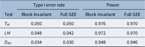
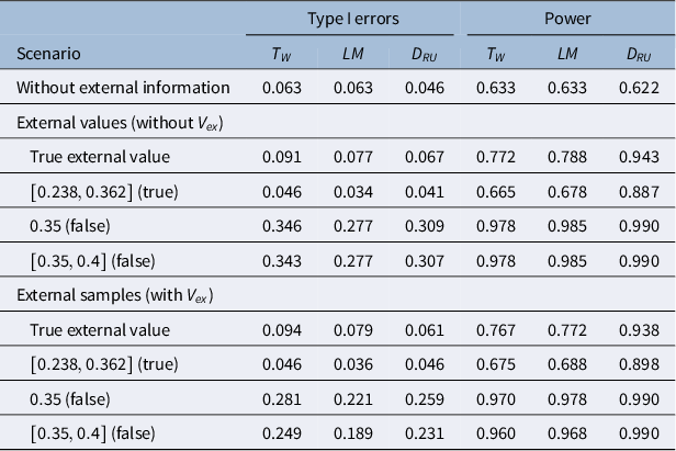
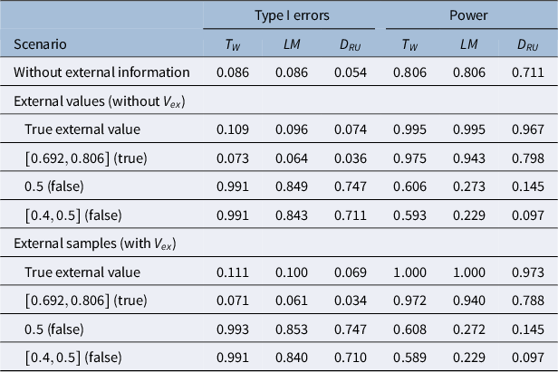

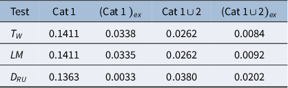


 Open access

