





1. Introduction
Stochastic orderings have served as a fundamental and versatile framework for comparing distributions of random variables, capturing a wide range of relationships relevant to diverse fields. Among these methods, stochastic dominance (SD) is particularly important in decision making under uncertainty, as it allows for ranking alternatives according to the risk preferences of decision makers [Reference Denuit, Dhaene, Goovaerts and Kaas6, Reference Müller and Stoyan22, Reference Shaked and Shanthikumar27].
At its core, SD involves two key components: the integral condition, which is the ordering rule based on distribution functions, and the utility class, which reflects the shared preferences of decision makers. One of the most well-known concepts in stochastic dominance, first-order stochastic dominance (FSD), ranks two alternatives based on the distribution functions F and G using the integral condition
 $ F(x) \geq G(x) $
for all
 $ x \in \mathbb{R} $
, denoted as
 $ F \preceq_{\mathrm{FSD}} G $
. This is equivalent to the condition
 $ \mathbb{E}_F[u] \leq \mathbb{E}_G[u] $
for all u within the utility class, consisting of all increasing functions for which the expectations exist. Similarly, the other widely used stochastic dominance relation, second-order stochastic dominance (SSD), states that G dominates F in SSD, denoted as
 $ F \preceq_{\mathrm{SSD}} G$
, if the integral condition
 $ 0 \leq \int_{-\infty}^{t} (F(x) - G(x)) \,{\mathrm{d}} x $
holds for all
 $ t \in \mathbb{R} $
. This condition is equivalent to
 $ \mathbb{E}_F[u] \leq \mathbb{E}_G[u] $
, where u belongs to the class of all increasing and concave utility functions.
A closer look immediately reveals a substantial gap between FSD and SSD. From a mathematical perspective, the integral condition of FSD is highly restrictive, as even a single violation at any point prevents the distributions from being ranked. This results in FSD having low discriminatory power. On the other hand, SSD does not hold when the functions fail to satisfy global concavity, as in the case of those with local non-concave segments. From a decision-theoretic perspective, these functions reflect the preferences of decision makers with mixed risk attitudes – for example, individuals who buy insurance while also engaging in gambling (see [Reference Friedman and Savage9], [Reference Markowitz20]).
The concept of interpolating between dominance rules originates with Fishburn [Reference Fishburn7], who utilized fractional integrals to define relations of any real order
 $\alpha\ge 1$
on bounded supports, a framework subsequently expanded in [Reference Fishburn8] to unbounded distributions through the necessary moment conditions. In a more recent development, the landmark paper by Müller et al. [Reference Müller, Scarsini, Tsetlin and Winkler23] introduced fractional stochastic dominance, which bridges FSD and SSD by incorporating a fixed parameter
 $\gamma \in [0, 1]$
.
Definition 1. (Fractional
 $(1+\gamma)$
-SD.) For fixed
 $\gamma\in [0, 1]$
, we say that G dominates F in the sense of fractional
 $(1+\gamma)$
-SD, denoted by
 $F \preceq_{(1+\gamma)\textrm{-SD}} G$
, if
 \begin{equation}\int_{-\infty}^{t} ( F(x) - G(x) )_{-}\,{\mathrm{d}} x \le \gamma \int_{-\infty}^{t} (F(x) - G(x) )_{+} \,{\mathrm{d}} x \quad \text{for all $t\in \mathbb{R}$,}\end{equation}
where for any real number z,
 $z_+\,:\!=\, \max\{z,0\}$
and
 $z_- \,:\!=\, \max\{ -z,0\}$
.
The utility counterpart of the relation
 $F \preceq_{(1+\gamma)\textrm{-SD}} G$
is as follows. For a given
 $\gamma\in [0, 1]$
,
 $F \preceq_{(1+\gamma)\textrm{-SD}} G$
if and only if
 $ \mathbb{E}_F[u] \leq \mathbb{E}_G[u] $
for every
 $u\in \mathscr{U\,}^{*}_{\gamma}$
, where
 \begin{equation}\mathscr{U\,}^{*}_{\gamma} \,:\!=\, \biggl\{ u\colon \mathbb{R} \to \mathbb{R} \colon0\leq \gamma \dfrac{u(x_4) -u(x_3)}{x_4-x_3} \leq \dfrac{u(x_2)-u(x_1)}{x_2-x_1}\ \text{for all}\ x_1 < x_2 \le x_3 < x_4 \biggr\}. \end{equation}
Specifically,
 $\gamma=0$
corresponds to FSD, while
 $\gamma=1$
aligns with SSD. For values of
 $\gamma \in (0,1)$
, the resulting fractional
 $(1+\gamma)$
-SD relaxes the integral condition of FSD, offering more informative criteria for ranking. Moreover, it expands the SSD utility class, consisting of a broader range of functions, including those with local non-concavities. This pivotal contribution has since served as a foundation for further research, inspiring a series of follow-up studies ([Reference Huang, Tzeng and Zhao10], [Reference Lando and Bertoli-Barsotti12], [Reference Mao and Wang17], [Reference Mao, Wu and Hu19], [Reference Müller, Scarsini, Tsetlin and Winkler24], [Reference Müller, Scarsini, Tsetlin and Winkler25], among others).
In this paper, motivated by the significant interest and the contributions of the fractional
 $(1+\gamma)$
-SD framework, we extend its capabilities by replacing the fixed coefficient
 $\gamma$
with a function
 $\unicode{x1D6C4}\colon \mathbb{R} \to [0, 1]$
. This introduces two distinct generalized families of fractional SD, depending on whether the extension takes place in the integral condition (1) or the utility class (2). The rest of this paper is organized as follows. In Section 2 we introduce multi-fractional stochastic dominance (MFSD) by extending the integral condition (1). We derive the corresponding utility class and prove an associated ‘if and only if’ theorem. We examine the consequences of this generalization and show that MFSD can effectively order distributions that cannot be ordered via fractional SD. In Section 3 we provide another generalized family of functional fractional stochastic dominance (FFSD) obtained from applying the functional extension on the utility side (2). We analyse the properties and implications, presenting an ‘if and only if’ theorem that connects the FFSD utility class to the integral condition. Additionally, we mathematically establish the key distinctions between FFSD and MFSD through their respective utility classes, supported by examples based on piecewise continuously differentiable functions. So far, the first two sections focus more on the mathematical aspects. Section 4 explores functional extensions within the decision-theoretic framework, focusing on the concept of partial greediness in both FFSD and MFSD. This novel measure quantifies how risk-taking behaviour varies with wealth. This variability enables the development of classification tools for both utility spaces. Additionally, we reveal a key relationship between the function
 $\unicode{x1D6C4}$
, partial greediness, and average risk aversion, providing a decision-theoretic interpretation for
 $\unicode{x1D6C4}$
. In Section 5 we follow an approach similar to previous sections in order to construct the generalized family of functional almost stochastic dominance. This framework extends the concept of almost stochastic dominance [Reference Leshno and Levy15]. Section 6 concludes the paper. All technical details and proofs are provided in the supplementary material.
2. Generalization through integral condition
In this section we introduce the multi-fractional stochastic dominance framework, explore its key features, and examine how the generalization via integral condition (1) extends the fractional
 $(1+\gamma)$
-SD framework.
2.1. MFSD: Definition
We begin by defining multi-fractional stochastic dominance.
Definition 2. (Multi-fractional
 $(1+\unicode{x1D6C4})$
-SD.) Let
 $\boldsymbol{ \gamma}\colon \mathbb{R} \to [0, 1]$
be an arbitrary non-decreasing bounded function. Let F and G be two arbitrary distribution functions. We say that G dominates F in the sense of the multi-fractional
 $(1+\boldsymbol{ \gamma})$
-SD, denoted by
 $F \preceq^{\mathrm{MF}}_{(1+\boldsymbol{ \gamma})\textrm{-SD}} G$
, if
 \begin{equation}\int_{-\infty}^{t} ( F(x) - G(x) )_{-}{\mathrm{d}} x \le \boldsymbol{ \gamma}(t) \int_{-\infty}^{t} (F(x) - G(x) )_{+} {\mathrm{d}} x \quad \text{for all $t\in \mathbb{R}$.}\end{equation}
Remark 1.
-
(i) Clearly the multi-fractional
 $(1+\unicode{x1D6C4})$
-SD coincides with the fractional
$(1+\gamma)$
-SD as soon as
$\boldsymbol{ \gamma}(t) =\gamma \in [0, 1]$
for every t. Furthermore, when, for some
$\gamma \in(0,1)$
, function
$\boldsymbol{ \gamma}(t) \leq \gamma$
for every
$t\in \mathbb{R}$
, then the multi-fractional
$(1+\unicode{x1D6C4})$
-SD implies the fractional
$(1+\gamma)$
-SD and, similarly, if the function
$\boldsymbol{ \gamma}(t) \geq \gamma$
for every
$t\in \mathbb{R}$
, then the fractional
$(1+\gamma)$
-SD implies the multi-fractional
$(1+\unicode{x1D6C4})$
-SD.
-
(ii) The non-decreasing nature of the function
$\unicode{x1D6C4}$
is not technically required but is crucial for defining a meaningful order relation. To elaborate this further, consider
$\unicode{x1D6C4}$
as a non-constant, non-increasing function. In this case, any value of
$\unicode{x1D6C4}$
other than its minimum will not influence the ordering of the distribution functions. This is because smaller values of
$\unicode{x1D6C4}$
impose stronger dominance rules. Consequently, the smallest value of
$\unicode{x1D6C4}$
dictates the order relation across the entire support of the distributions. -
(iii) By our assumptions, the function
$\unicode{x1D6C4}$
is non-decreasing and bounded, hence it has at most countably many discontinuities of the first kind, and clearly
$\unicode{x1D6C4} (t) \le \unicode{x1D6C4}(t^+)$
for each t. Therefore, due to continuity of the integral operator, without of loss of generality, one can always assume that the function
$\unicode{x1D6C4}$
is always right-continuous. This desirable feature allows us to add one extra layer of randomness to the multi-fractional stochastic dominance framework by considering
$\unicode{x1D6C4}$
as a distribution function (see Example 6). We expect that such a desirable viewpoint will provide us with extra strengths that can be useful in certain applications.





As noted, the function
 $\unicode{x1D6C4}$
encodes local relationships between the distributions. Accordingly, multi-fractional
 $(1+\unicode{x1D6C4})$
-SD exhibits a form of local interpolation. We now provide an alternative characterization of multi-fractional
 $(1+\unicode{x1D6C4})$
-SD that rigorously formalizes this local interpolation property and clarifies its precise interpretation motivated by the classical work [Reference Atkinson2].
Definition 3. (Restricted fractional
 $(1+\gamma)_{t}^r$
-SD.) For fixed
 $\gamma\in [0, 1]$
and given
 $t\in \mathbb{R}$
, we say that G dominates F in the sense of restricted fractional
 $(1+\gamma)_{t}^r$
-SD, denoted by
 $F \preceq_{(1+\gamma)_{t}^r\textrm{-SD}} G$
, if
 \begin{equation*} \int_{-\infty}^{s} ( F(x) - G(x) )_{-}{\mathrm{d}} x \le \gamma \int_{-\infty}^{s} (F(x) - G(x) )_{+} {\mathrm{d}} x \quad \text{for all $s \le t$.}\end{equation*}
Proposition 1. Let
 $\boldsymbol{ \gamma}\colon \mathbb{R} \to [0, 1]$
be an arbitrary non-decreasing function. Then
 $F \preceq^{\mathrm{MF}}_{(1+\boldsymbol{ \gamma})\textrm{-SD}} G$
if and only if
 $F \preceq_{(1+\boldsymbol{ \gamma}(t))_{t}^r\textrm{-SD}} G$
for all
 $t\in \mathbb{R}$
.
Example 1. (Local interpolation.) Let
 $\gamma\in(0,1)$
be a constant. Consider the following non-decreasing function:
 \begin{equation*}\boldsymbol{ \gamma}(t)=\begin{cases}0 & \text{if $ t \le t_1$,} \\\gamma & \text{if $ t_1 < t \leq t_2$,} \\1 & \text{if $ t>t_2$,} \end{cases}\end{equation*}
where
 $t_1<t_2$
are real numbers. Assume that
 $F \preceq^{\mathrm{MF}}_{ (1+ \boldsymbol{ \gamma})\textrm{-SD}} G$
. Then
 $\boldsymbol{ \gamma}(t_1)=0$
entails that
 $F \preceq_{(1+\boldsymbol{ \gamma}(t_1))^r_{t_1}\textrm{-SD}} G$
, i.e.
 $F(x) \ge G(x)$
for all
 $x \le t_1$
. Similarly, the condition
 $\boldsymbol{ \gamma}(t_2)=\gamma$
yields that
 $F \preceq_{(1+\gamma)^r_{t_2}\textrm{-SD}} G$
, that is,
 $F \preceq_{(1+\gamma)\textrm{-SD}} G$
holds on the interval
 $(\!-\infty, t_2]$
. Lastly, the fact that
 $\boldsymbol{ \gamma}(t) =1$
, for all
 $t \in (t_2,\infty)$
, implies that
 $F \preceq_{\mathrm{SSD}} G$
. Hence, with appropriately chosen non-decreasing function
 $\boldsymbol{ \gamma}$
, one can simultaneously order given F and G from first (strongest) to second (weakest) order on different portions (capture with function
 $\boldsymbol{ \gamma}$
) of the supports.
Now we discuss yet another feature of the MFSD framework. It is known that the assumption of equal means for the distribution functions (
 $\mu_F=\mu_G$
) renders them indistinguishable in terms of the fractional
 $(1 + \gamma)$
-SD, for any constant
 $\gamma \in [0, 1)$
. We exclude the limiting case
 $\gamma=1$
due to the fact that it corresponds to (less interesting) SSD. Nonetheless, as demonstrated in the following example, the multi-fractional
 $(1+\unicode{x1D6C4})$
-SD can effectively order distributions with equal means, provided that an appropriate function, i.e. non-constant and satisfying
 $\boldsymbol{ \gamma}(t)=1$
for some
 $t\in \mathbb{R}$
, is chosen.
Example 2. Consider
 $G \sim \delta_{\mu} $
(the Dirac measure at the point
 $\mu\in \mathbb{R}$
), and the distribution functions
 \begin{equation*}F(x)=\begin{cases}0 & \text{if $ x < \mu-\varepsilon$,} \\1/2 & \text{if $ \mu-\varepsilon \le x < \mu+\varepsilon$,}\\1 & \text{if $ \mu+\varepsilon \le x$,}\end{cases} \quad \text{and} \quad \unicode{x1D6C4}(t)=\begin{cases}0 & \text{if $ \mu-\varepsilon\le t \le \mu$,} \\{{(t-\mu)}/{ \varepsilon}} & \text{if $ \mu< t <\mu+\varepsilon$,}\\1 & \text{if $ \mu+\varepsilon\le t$,}\end{cases}\end{equation*}
where
 $\mu>\varepsilon>0$
. The straightforward calculation shows that the integral condition (3) holds. Hence
 $F \preceq^{\mathrm{MF}}_{(1+\unicode{x1D6C4})\textrm{-SD}} G$
. However,
 $F \npreceq_{ (1+ \gamma)\textrm{-SD}} G$
for any constant
 $\gamma \in [0,1)$
, since the inequality (1) fails at
 $t=\mu+\varepsilon$
,
 \begin{align*}0=\mu_G-\mu_F=\int_{\mu-\varepsilon}^{\mu+\varepsilon} ( F(x)-G(x) )_+ {\mathrm{d}} x - \int_{\mu-\varepsilon}^{\mu+\varepsilon} ( F(x)-G(x) )_- {\mathrm{d}} x.\end{align*}
In contrast, we have
 $\boldsymbol{ \gamma}(\mu+\varepsilon)=1$
.
We can readily construct an additional example that extends Example 2 to a scenario beyond identical means. However, to avoid redundancy, we will not pursue this further. The following example, though rather technical, examines the non-trivial relationship between fractional and multi-fractional SD rules. While we provide the example here for context, the explicit constructions are provided in the supplementary material to avoid disrupting the flow.
Example 3. The purpose of the example is to show that for any given constant
 $\gamma \in (0,1)$
and every (non-decreasing) function
 $\boldsymbol{ \gamma}$
satisfying
 $\boldsymbol{ \gamma}(t^0) < \gamma < \boldsymbol{ \gamma}(t_0)$
for some
 $t^0<t_0$
, there exist distribution functions F and G so that either one of the following holds:
-
(i)
$F \preceq^{\mathrm{MF}}_{ (1+ \boldsymbol{ \gamma})\textrm{-SD}} G$
but
$F \npreceq_{(1+\gamma)\textrm{-SD}} G$
, -
(ii)
$F \npreceq^{\mathrm{MF}}_{ (1+ \boldsymbol{ \gamma})\textrm{-SD}} G$
but
$F \preceq_{(1+\gamma)\textrm{-SD}} G$
.


The full details of the construction are provided in the supplementary material.
The conclusion is that in both non-trivial scenarios, one can always construct two distribution functions F and G that are not distinguishable by the fractional
 $(1+\gamma)$
-SD but it is possible to order them with the multi-fractional
 $(1+\unicode{x1D6C4})$
-SD, and vice versa.
Example 4. In this example we visualize the function
 $t\mapsto \unicode{x1D6C4}(t)$
to show how it changes under perturbations of one distribution within a location–scale family; this provides a visual counterpart to Example 2.11 of [Reference Müller, Scarsini, Tsetlin and Winkler23] in our setting. Let F and G be from the same location–scale family,
 \[F(x)=H\biggl(\frac{x-\mu_F}{\sigma_F}\biggr)\quad \text{and}\quad G(x)=H\biggl(\frac{x-\mu_G}{\sigma_G}\biggr),\]
where H denotes the standard normal CDF. Write
 $\Delta\mu\,:\!=\, \mu_G-\mu_F$
and
 $\Delta\sigma\,:\!=\, \sigma_F-\sigma_G$
. Under
 $\mu_F\le \mu_G$
and
 $\sigma_G<\sigma_F$
, the pair (F,G) is single-crossing with crossing point
 $t_1=\mu_F+\sigma_F{{\Delta\mu}/{\Delta\sigma}}$
. In this regime, the strongest MFSD ordering is obtained by the smallest admissible degree function, denoted
 $\unicode{x1D6C4}_{\min}(F,G)$
, which one can derive as
 \begin{equation*} \unicode{x1D6C4}_{\min}(F,G)(t)=\begin{cases}0, & t\le t_1,\\\dfrac{\Delta \sigma \displaystyle\int_{\Delta \mu/\Delta \sigma}^{(t-\mu_F)/\sigma_F} ( 1 - H (z) )\,{\mathrm{d}} z- \sigma_G \int_{(t-\mu_F)/\sigma_F}^{(t-\mu_G)/\sigma_G} ( 1 - H (z) )\,{\mathrm{d}} z}{\Delta\sigma \displaystyle\int_{-\infty}^{\Delta \mu/\Delta \sigma} H(z)\,{\mathrm{d}} z},& t>t_1.\end{cases}\end{equation*}
For plotting, fix
 $F=\mathcal N(0,1)$
(so
 $\mu_F=0$
,
 $\sigma_F=1$
), and
 $G=\mathcal N(\mu_G,\sigma_G^2)$
with
 $\Delta\mu=\mu_G$
and
 $\Delta\sigma=1-\sigma_G$
. We perturb G over a grid of
 $(\mu_G,\sigma_G)$
summarized by the ratio
 $\Delta\mu/\Delta\sigma=\mu_G/(1-\sigma_G)$
. The resulting surface
 $(t,\Delta\mu/\Delta\sigma)\mapsto \unicode{x1D6C4}_{\min}(F,G)(t)$
(and its contours/slices) makes the interpretation transparent,
 $\unicode{x1D6C4}_{\min}(t)=0$
up to the crossing point
 $t_1=\mu_G/(1-\sigma_G)$
, and larger perturbations (larger
 $\Delta\mu/\Delta\sigma$
) shift the crossing point
 $t_1$
to the right and keep
 $\unicode{x1D6C4}_{\min}(t)$
closer to 0 over a wider range of t. Holding t fixed,
 $\unicode{x1D6C4}_{\min}(F,G)(t)$
falls quickly toward zero as
 $\Delta\mu/\Delta\sigma$
increases, indicating that stronger perturbations push the maximal admissible MFSD degree toward the FSD limit while weaker perturbations move it towards the SSD limit. Higher values of t shift the curve upward, since
 $\unicode{x1D6C4}_{\min}$
is non-decreasing in t and therefore attains larger values.
Normal location–scale perturbations with
 $F=\mathcal N(0,1)$
and
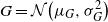 $G=\mathcal N\bigl(\mu_G,\sigma_G^2\bigr)$
. (a) Fixed-
 $\Delta\mu/\Delta\sigma$
slices. (b) Fixed-t slices. (c) Surface.

Figure 1 Long description
Panel A: This line graph shows the relationship between t and gamma_min(F,G)(t) for different values of delta_mu/delta_sigma. The x-axis represents t, and the y-axis represents gamma_min(F,G)(t). The graph includes multiple lines representing different values of delta_mu/delta_sigma (0, 0.5, 1, 2, 3). The lines show how gamma_min(F,G)(t) changes with t for each value of delta_mu/delta_sigma. Panel B: This line graph shows the relationship between delta_mu/delta_sigma and gamma_min(F,G)(t) for different values of t. The x-axis represents delta_mu/delta_sigma, and the y-axis represents gamma_min(F,G)(t). The graph includes multiple lines representing different values of t (0.5, 1, 2, 4). The lines show how gamma_min(F,G)(t) changes with delta_mu/delta_sigma for each value of t. Panel C: This 3D surface plot shows the relationship between delta_mu/delta_sigma, t, and gamma_min(F,G)(t). The x-axis represents delta_mu/delta_sigma, the y-axis represents t, and the z-axis represents gamma_min(F,G)(t). The surface plot illustrates how gamma_min(F,G)(t) varies with both delta_mu/delta_sigma and t.
2.2. The MFSD universe
In this section we formalize all prior observations within a structured framework. For every constant
 $\gamma \in [0, 1]$
and non-decreasing function
 $\boldsymbol{ \gamma }\colon \mathbb{R} \to [0, 1]$
, we introduce
 \begin{align*}\unicode{x1D4D4}_{{F}}(\gamma) & \,:\!=\, \{ (F,G) \in \unicode{x1D4D3}\,(\mathbb{R}) \times \unicode{x1D4D3}\,(\mathbb{R}) \colon F \preceq_{(1+\gamma)\textrm{-SD}} G \},\\\unicode{x1D4D4}_{\mathrm{MF}}(\boldsymbol{ \gamma}) & \,:\!=\, \bigr\{ (F,G) \in \unicode{x1D4D3}\,(\mathbb{R}) \times \unicode{x1D4D3}\,(\mathbb{R}) \colon F \preceq^{\mathrm{MF}}_{ (1+ \boldsymbol{ \gamma})\textrm{-SD}} G \bigr\},\end{align*}
where
 $\unicode{x1D4D3}\,(\mathbb{R})$
is the set of all distribution functions supported on
 $\mathbb{R}$
. Also, we denote
 $\unicode{x1D4D4}_{{F}}(1) = \unicode{x1D4D4}_{\mathrm{SSD}}$
. Note that, clearly, we have the set identity
 $ \unicode{x1D4D4}_{\mathrm{MF}}(\boldsymbol{ \gamma}) = \unicode{x1D4D4}_{{F}}(\gamma)$
as soon as
 $\unicode{x1D6C4} \equiv \gamma$
is the constant function, and furthermore, when
 $ \boldsymbol{ \gamma} (t ) \ge \gamma$
 $(\boldsymbol{ \gamma} (t ) \le \gamma)$
for every
 $t \in \mathbb{R}$
, the set inclusion
 $ \unicode{x1D4D4}_{{F}}(\gamma) \, \subsetneq \, \unicode{x1D4D4}_{\mathrm{MF}}(\boldsymbol{ \gamma})$
 $( \unicode{x1D4D4}_{\mathrm{MF}}(\boldsymbol{ \gamma}) \, \subsetneq \, \unicode{x1D4D4}_{{F}}(\gamma))$
holds. Lastly, Example 3 shows that for every constant
 $\gamma \in (0,1)$
and every (non-decreasing) function
 $\boldsymbol{ \gamma}$
satisfying
 $\boldsymbol{ \gamma}(t^0) < \gamma < \boldsymbol{ \gamma}(t_0)$
for some
 $t^0<t_0$
, we have
 \begin{equation*}\unicode{x1D4D4}_{\mathrm{MF}}(\boldsymbol{ \gamma}) \setminus \unicode{x1D4D4}_{{F}}(\gamma) \neq \emptyset \quad \text{and} \quad \unicode{x1D4D4}_{{F}}(\gamma) \setminus \unicode{x1D4D4}_{\mathrm{MF}}(\boldsymbol{ \gamma}) \neq \emptyset .\end{equation*}
Before proceeding further, for notational convenience throughout this paper, we use the following notation for the limits of a non-decreasing function
 $\unicode{x1D6C4}$
. We define
 \[{\stackrel{\rule{.6em}{1.5pt}}{\unicode{x1D6C4}}}\,:\!=\, \lim_{t\to +\infty}\boldsymbol{ \gamma}(t)=\sup\nolimits_{t\in\mathbb{R}}\unicode{x1D6C4}(t) \quad \text{and} \quad \raise-4.8pt\hbox{$\buildrel \displaystyle\unicode{x1D6C4} \over {\rule{.6em}{1.5pt}}$} \,:\!=\, \lim_{t\to -\infty}\boldsymbol{ \gamma}(t)=\inf_{t \in \mathbb{R}} \unicode{x1D6C4}(t).\]
The next result aims to summarize the non-trivial relations between the corresponding universes.
Theorem 1. Let
 $\boldsymbol{ \gamma}\colon \mathbb{R}\rightarrow [0, 1]$
be an arbitrary non-decreasing function. Then the following statements hold.
-
(a) The inclusions
$\unicode{x1D4D4}_{{F}}(\raise-4.8pt\hbox{$\buildrel \displaystyle\unicode{x1D6C4} \over {\rule{.6em}{1.5pt}}$} \subseteq \unicode{x1D4D4}_{\mathrm{MF}}(\boldsymbol{ \gamma}) \subseteq \unicode{x1D4D4}_{{F}}({\stackrel{\rule{.6em}{1.5pt}}{\unicode{x1D6C4}}})$
hold and are strict as soon as
$\boldsymbol{ \gamma}$
is a non-constant function. -
(b) The corresponding universes associated to fractional and multi-fractional stochastic dominances coincide with
$\unicode{x1D4D4}_{\mathrm{SSD}}$
, namely that (4)In addition, if the non-interesting case, i.e.
\begin{align}\bigcup_{ \gamma \in[0, 1] } \unicode{x1D4D4}_{{F}}(\gamma) =\bigcup_{ {\substack{ \boldsymbol{ \gamma}\colon \mathbb{R} \to [0, 1] \\{non\text{-}decreasing} } } } \, \unicode{x1D4D4}_{\mathrm{MF}}(\boldsymbol{ \gamma}) = \unicode{x1D4D4}_{\mathrm{SSD}}.\end{align}
$\boldsymbol{ \gamma}\equiv\gamma=1$
, is excluded from both sides, then the relation (4) reduces to
\begin{equation*} \bigcup_{ \gamma \in[0,1) } \unicode{x1D4D4}_{{F}}(\gamma) \subsetneq\bigcup_{ {\substack{ \boldsymbol{ \gamma}\colon \mathbb{R} \to [0, 1] \\{non\text{-}decreasing} \\\boldsymbol{ \gamma} \not\equiv 1 } } } \, \unicode{x1D4D4}_{\mathrm{MF}}(\boldsymbol{ \gamma}) = \unicode{x1D4D4}_{\mathrm{SSD}}.\end{equation*}



Remark 2. Part (b) of Theorem 1 demonstrates a significant feature of multi-fractional stochastic dominance in the sense that by removing the constant function
 $\boldsymbol{ \gamma}\equiv\gamma=1$
(corresponding to the SSD case), the universe of multi-fractional stochastic dominance remains as large as that of SSD, whereas this is not the case for fractional stochastic dominance.
2.3. Utility class
In this section we first introduce the set of utility functions that generates the multi-fractional SD. Then we prove the ‘if and only if’ theorem between the introduced utility class and the integral condition (3). As mentioned previously, the utility class corresponding to MFSD is not readily available. Therefore the definition requires preliminary steps to be established. As our starting point, we present the following simple lemma and the subsequent proposition, inspired by the fractional SD utility space
 $\mathscr{U\,}^*_{\gamma}$
and by [Reference Müller, Scarsini, Tsetlin and Winkler23, Theorem 2.4] (specifically, direction (b)).
Lemma 1. Let
 $\boldsymbol{ \gamma}\,:\, \mathbb{R} \rightarrow [0, 1]$
be an arbitrary non-decreasing function. For each
 $t \in \mathbb{R}$
, we consider the following function space:
 \begin{align*} \mathscr{U\,}^{t}_{\boldsymbol{ \gamma}(t)}&\,:\!=\, \biggl\{ u\colon \mathbb{R} \to \mathbb{R}\colon u(x)=u(t) \ \ {for\, all}\ \, x \ge t \ \, {and} \notag \\&\qquad {for\, all}\,\,\ x_1 < x_2 \le x_3 < x_4, \, 0\leq \boldsymbol{ \gamma}(t) \dfrac{u(x_4) -u(x_3)}{x_4-x_3} \leq \dfrac{u(x_2)-u(x_1)}{x_2-x_1} \biggr\}.\end{align*}
Let F and G be two arbitrary distribution functions. For every
 $t \in \mathbb{R}$
, define the continuous function
 $u_t$
via its right-derivative
 \begin{equation}u_t^{\prime}(x)=\begin{cases}\boldsymbol{ \gamma}(t) & {if \, G(x) \le F(x)\, and \, x \leq t,} \\1 & {if \, F(x) < G(x)\, and \, x \leq t\,,} \\0 & {if \, t < x\,.}\end{cases}\end{equation}
Then
 $u_t \in \mathscr{U\,}^{t}_{\boldsymbol{ \gamma}(t)}\,$
for every
 $t \in \mathbb{R}$
.
Proposition 2. Let F and G be two arbitrary probability distributions having finite means, and let
 $\boldsymbol{ \gamma}\colon \mathbb{R} \rightarrow [0, 1]$
be a non-decreasing function. Then relation
 \begin{equation*} \mathbb{E}_F[u_t] \le \mathbb{E}_G [u_t] \quad {for\, all \, t \in \mathbb{R}}\end{equation*}
implies that
 $F \preceq^{\mathrm{MF}}_{(1+\boldsymbol{ \gamma})\textrm{-SD}} G$
.
The conclusion is that any desirable utility class for MFSD should contain the family of those base-type functions
 $\{u_t \colon t \in \mathbb{R}\}$
given in (5). Observe that these functions enjoy two important characteristics.
-
(i) They are constant over the region
$(t,+\infty)$
and hence their derivatives vanish (this in particular implies that there is no contribution to the expected value via the integration by parts formula). -
(ii) On the complementary range
$(\!-\infty,t)$
they should manifest the fractional
$(1+\gamma)$
-SD base-type functions with
$\unicode{x1D6C4}(t)$
instead of a fixed parameter
$\gamma$
.


Based on the discussion thus far, we take the function spaces
 $\mathscr{U\,}^{t}_{\boldsymbol{ \gamma}(t)}$
for
 $t \in \mathbb{R}$
as the building blocks of the MFSD utility class. Before proceeding, let us summarize some of the key mathematical properties that are crucial for the subsequent discussion.
Proposition 3. Let
 $\boldsymbol{ \gamma}\colon \mathbb{R}\rightarrow [0, 1]$
be an arbitrary non-decreasing function and let
 $t \in \mathbb{R}$
.
-
(a) Every
$u\in \mathscr{U\,}^{t}_{\boldsymbol{ \gamma}(t)}$
is bounded from above (in fact
$u(x) =u(t)$
for all
$x \ge t$
) and is a non-decreasing function, hence differentiable almost everywhere. -
(b) Suppose
$ \boldsymbol{ \gamma}(t) \neq 0 $
. Then every function
$ u\in \mathscr{U\,}^{t}_{\boldsymbol{ \gamma}(t)} $
is continuous on
$\mathbb{R}$
and Lipschitz-continuous on any interval of the form
$ [a,\infty) $
. Consequently, it is absolutely continuous on every compact interval of
$\mathbb{R}$
. -
(c) Let
$\unicode{x1D6C4}(t)<1$
and Then
\begin{equation*} \widetilde{\mathscr{U\,}}^{t}_{\unicode{x1D6C4}(t)}\,:\!=\, \bigl\{u\in \mathscr{U\,}^{t}_{\unicode{x1D6C4}(t)}\colon {u_-'(x)\, and \, u_+'(x)\, exist\, for\, all \, x \in\mathbb{R}} \bigr\}.\end{equation*}
$\widetilde{\mathscr{U\,}}^{t}_{\unicode{x1D6C4}(t)} \subsetneq \mathscr{U\,}^{t}_{\unicode{x1D6C4}(t)}$
.
-
(d) The class
$\mathscr{U\,}_{\boldsymbol{ \gamma}(t)}^t$
is a convex cone and closed in the topology of pointwise convergence. -
(e) Let
$ s \le t$
. Then the following set inclusions are in place:
\begin{equation*}\mathscr{U\,}^s_{\unicode{x1D6C4}(t)} \subseteq \mathscr{U\,}^t_{\unicode{x1D6C4}(t)} \quad \textit{and} \quad \mathscr{U\,}^s_{\unicode{x1D6C4}(t)} \subseteq \mathscr{U\,}^s_{\unicode{x1D6C4}(s)}.\end{equation*}
-
(f) Limit
$\displaystyle{\lim_{t\rightarrow -\infty }\mathscr{U\,}^t_{\unicode{x1D6C4}(t)}}$
as
$t \to -\infty$
exists, and moreover,
\begin{equation*}\displaystyle{\lim_{t\rightarrow -\infty }\mathscr{U\,}^t_{\unicode{x1D6C4}(t)}}\,=\!:\, \mathscr{U\,}^{-\infty}_{\!\substack{{\unicode{x1D6C4}}\\\rule{.6em}{1.5pt}}} =\{{constant\, functions}\}.\end{equation*}
-
(g) Limit
$\displaystyle{\lim_{t\rightarrow \infty }\mathscr{U\,}^t_{\unicode{x1D6C4}(t)}}$
as
$t \to +\infty$
exists, and moreover, where
\begin{equation*}\lim_{t\rightarrow \infty }\mathscr{U\,}^t_{\unicode{x1D6C4}(t)}=\mathscr{U\,}^{+\infty}_{\stackrel{\rule{.6em}{1.5pt}}{\unicode{x1D6C4}}}{,}\end{equation*}
\[\mathscr{U\,}^{+\infty}_{\stackrel{\rule{.6em}{1.5pt}}{\unicode{x1D6C4}}} \,:\!=\, \biggl\{ u \colon 0 \le {\stackrel{\rule{.6em}{1.4pt}}{\unicode{x1D6C4}}} \dfrac{u(x_4) -u(x_3)}{x_4-x_3} \leq \dfrac{u(x_2)-u(x_1)}{x_2-x_1} \ for\ all\ x_1 < x_2 \le x_3 < x_4\biggr\}=\mathscr{U\,}^{*}_{\stackrel{\rule{.6em}{1.5pt}}{\unicode{x1D6C4}}}.\]


For each
 $t \in \mathbb{R}$
, the class
 $\mathscr{U\,}^{t}_{\boldsymbol{ \gamma}(t)}$
contains (utility) functions with a limited variety of characteristics. Therefore, by gathering spaces
 $\mathscr{U\,}^{t}_{\boldsymbol{ \gamma}(t)}$
for all
 $t\in [\!-\infty,\infty]$
, one can create a larger class which contains a broader range of utility functions with different attributes. Define
 \begin{equation*} \mathscr{U\,}^{\mathrm{Union}}_{\unicode{x1D6C4}}\,:\!=\, \bigcup_{t\in [\!-\infty,\infty]}\mathscr{U\,}^t_{\unicode{x1D6C4}(t)}.\end{equation*}
In the above, for technical reasons, when
 $\unicode{x1D6C4}(t)=0$
, we restrict the utility space
 $\mathscr{U\,}^{t}_{\unicode{x1D6C4}(t)}$
to consist of non-decreasing continuous functions. As follows from Proposition 3(d), although for each
 $t \in [\!-\infty,\infty]$
the class
 $\mathscr{U\,}^t_{\unicode{x1D6C4}(t)}$
is a convex cone, however,
 $\mathscr{U\,}^{\mathrm{Union}}_{\unicode{x1D6C4}}$
is not necessarily closed under (arbitrary) addition. Given that the sum of utility functions naturally produces a new utility function, and considering the linearity of expected utilities, the class
 $\mathscr{U\,}^{\mathrm{Union}}_{\unicode{x1D6C4}}$
alone is not a useful candidate for the utility class of the multi-fractional
 $(1+\unicode{x1D6C4})$
-SD. However, it is simple to overcome the latter issue by considering all the possible positive (finite) linear combinations. Hence we finally introduce the following (utility) class.
Definition 4. (Utility class of MFSD.) Let
 $\boldsymbol{ \gamma}\colon \mathbb{R} \rightarrow[0, 1]$
be an arbitrary non-decreasing function. A (utility) class for the multi-fractional
 $(1+\unicode{x1D6C4})$
-SD is defined as
 \begin{equation*} \mathscr{U\,}^{\mathrm{MF}}_{\unicode{x1D6C4}} \,:\!=\, \operatorname{span}_{\mathbb{R}_+} \bigl\{u \colon u\in \mathscr{U\,}^{\mathrm{Union}}_{\unicode{x1D6C4}} \bigr\} = \Biggl\{ u = \sum_{\text{finite}} \lambda_k u_k, \, \lambda_k \ge 0, \, u_k \in \mathscr{U\,}^{\mathrm{Union}}_{\unicode{x1D6C4}} \Biggr\}.\end{equation*}
Now we are ready to state the main theorem of this section.
Theorem 2. Let
 $\boldsymbol{ \gamma}\colon \mathbb{R} \rightarrow[0, 1]$
be an arbitrary non-decreasing function. For every two distribution functions F and G, the following statements are equivalent:
-
(a)
$F \preceq^{\mathrm{MF}}_{(1+\boldsymbol{ \gamma})\textrm{-SD}} G$
, -
(b)
$\mathbb{E}_F[u]\leq \mathbb{E}_G[u]$
for every
$u \in \mathscr{U\,}^{\mathrm{MF}}_{\unicode{x1D6C4}}$
.


Following the main theorem, we provide the next remark to emphasize several important points.
Remark 3.
-
(i) Clearly, if the non-decreasing function
$\boldsymbol{ \gamma}\equiv\gamma \in [0, 1]$
is constant, then
$\mathscr{U\,}^{\mathrm{MF}}_{\unicode{x1D6C4}}= \mathscr{U\,}^{*}_{\gamma}$
. In addition, for a non-decreasing function
$\unicode{x1D6C4}$
, the inclusions hold and both inclusions are strict when
\begin{equation*}\mathscr{U\,}^{*}_{\stackrel{\rule{.6em}{1.5pt}}{\unicode{x1D6C4}}} \subseteq \,\mathscr{U\,}^{\mathrm{MF}}_{\unicode{x1D6C4}} \, \subseteq \mathscr{U\,}^{*}_{\!\substack{{\unicode{x1D6C4}}\\\rule{.6em}{1.5pt}}}\end{equation*}
$\unicode{x1D6C4}$
is non-constant (see Theorem 1(a)). From the utility theory perspective, the second set inclusion means that
$\mathscr{U\,}^{\mathrm{MF}}_{\unicode{x1D6C4}}$
provides us with a more informative class compared to
$\mathscr{U\,}^{*}_{\!\substack{{\unicode{x1D6C4}}\\\rule{.6em}{1.5pt}}}$
. However, the first inclusion implies that the utility class
$\mathscr{U\,}^{\mathrm{MF}}_{\unicode{x1D6C4}}$
represents the preferences of a broader class of decision makers.
-
(ii) Due to the linear structure of
$\mathscr{U\,}^{\mathrm{MF}}_{\unicode{x1D6C4}}$
and, for every t, observing that
$\mathscr{U\,}^{t}_{\unicode{x1D6C4}(t)} \subsetneq \mathscr{U\,}^{*}_{\unicode{x1D6C4}(t)} $
, while multi-fractional
$(1+\unicode{x1D6C4})$
-SD establishes stochastic dominance over
$\mathscr{U\,}^{\mathrm{MF}}_{\unicode{x1D6C4}}$
, it is possible that no dominance (in the sense of fractional SD) holds in any
$\mathscr{U\,}^*_\gamma$
for all
$\gamma < {\stackrel{\rule{.6em}{1.5pt}}{\unicode{x1D6C4}}}$
. -
(iii) For a given parameter
$\gamma$
, one can choose a function
$\unicode{x1D6C4}\colon \mathbb{R}\to [0,\gamma]$
to further expand the set from
$\mathscr{U\,}^*_\gamma$
to
$\mathscr{U\,}^{\mathrm{MF}}_{\unicode{x1D6C4}}$
. This will ensure that individuals in
$\mathscr{U\,}^*_\gamma$
also agree on the ordering of random variables under
$(1+\unicode{x1D6C4})$
-SD, since
$\mathscr{U\,}^*_\gamma \subsetneq\mathscr{U\,}^{\mathrm{MF}}_{\unicode{x1D6C4}}$
. Similarly, choosing a function
$\unicode{x1D6C4}\colon \mathbb{R}\to [\gamma,1]$
will result in a smaller set of decision makers,
$\mathscr{U\,}^{\mathrm{MF}}_{\unicode{x1D6C4}} \subsetneq \mathscr{U\,}^*_\gamma$
, who unanimously agree on the ordering of random variables in the
$(1+\gamma)$
-SD sense. Hence MFSD can be utilized to further interpolate between FSD and
$(1+\gamma)$
-SD by choosing a function
$\unicode{x1D6C4}\colon \mathbb{R}\to [0,\gamma]$
, or between
$(1+\gamma)$
-SD and SSD by choosing a function
$\unicode{x1D6C4}\colon \mathbb{R}\to [\gamma,1]$
.


Next we continue with a few illustrating examples to gain a better understanding of the utility class.
Example 5. Let
 $\gamma_1 < \gamma_2 < \cdots < \gamma_n $
be n real numbers belonging to the interval [0, 1]. Consider the function
 \begin{equation}\unicode{x1D6C4} (t) =\begin{cases}\gamma_1 & \text{if $ t \le t_1$,}\\\gamma_2 & \text{if $ t_1\! \lt t \le t_2$,}\\\vdots\\\gamma_{n-1} & \text{if $ t_{n-2} < t \le t_{n-1}$,}\\\gamma_n & \text{if $ t > t_{n-1}$.}\end{cases}\end{equation}
Then we have
 \begin{align*}\mathscr{U\,}^{\mathrm{Union}}_{\unicode{x1D6C4}} = \Biggl( \bigcup_{k=1}^{n-1} \mathscr{U\,}^{\,t_k}_{\unicode{x1D6C4}(t_{k})} \Biggr) \bigcup \mathscr{U\,}^{+\infty}_{\stackrel{\rule{.6em}{1.5pt}}{\unicode{x1D6C4}}} =\Biggl( \bigcup_{k=1}^{n-1} \mathscr{U\,}^{\,t_k}_{\gamma_k} \Biggr) \bigcup \mathscr{U\,}^{*}_{\gamma_n},\end{align*}
where the function class
 $\mathscr{U\,}^{*}_{\gamma_n}$
corresponds to the fractional
 $(1+\gamma_n)$
-SD.
The purpose of the following example is to provide yet another capability of multi-fractional SD through its utility space.
Example 6. On certain occasions we require a given family of utility functions sharing particular features to belong to a single utility space, corresponding to a given SD rule. Next we construct a parametrized family
 $\mathscr{U\,}_{\Theta}$
of utility functions such that the only fractional utility space
 $\mathscr{U\,}^{*}_{\gamma}$
(associated with fractional
 $(1+\gamma)$
-SD) that contains
 $\mathscr{U\,}_{\Theta}$
is the first-order stochastic dominance (FSD) space, i.e.
 $\gamma=0$
. By contrast,
 $\mathscr{U\,}_{\Theta}$
can be embedded in a multi-fractional utility space
 $\mathscr{U\,}^{\mathrm{MF}}_{\unicode{x1D6C4}}$
that is a strict subset of the FSD utility space
 $\mathscr{U\,}_{0}$
, thereby yielding a stochastic dominance criterion under which a larger class of distribution functions can be ordered.
Let
 $\theta^* >0$
be fixed. Let
 $\Theta = (\theta^*,\infty)$
and consider a function
 $\widetilde{\unicode{x1D6C4}} \colon \Theta \to (0,1]$
so that (i) it is non-decreasing, (ii)
 $\widetilde{\unicode{x1D6C4}} (\theta) < \theta $
for every
 $\theta \in \Theta$
, and (iii)
 $\lim_{\theta \to \theta^*} \widetilde{\unicode{x1D6C4}} (\theta) =0$
. For every
 $\theta \in \Theta $
, we define a utility function
 $u_\theta$
via its right-derivative as
 \begin{equation*}u'_\theta (x) =\begin{cases}2 \widetilde{\unicode{x1D6C4}} (\theta)& \text{if $ x \le \widetilde{\unicode{x1D6C4}} (\theta)$,}\\1 + \widetilde{\unicode{x1D6C4}} (\theta)& \text{if $ \widetilde{\unicode{x1D6C4}} (\theta) < x \le \theta$,}\\\widetilde{\unicode{x1D6C4}} (\theta) & \text{if $ x > \theta$.}\end{cases}\end{equation*}
Then it is simple to observe that
 $u_\theta \in \mathscr{U\,}^*_{\widetilde{\unicode{x1D6C4}}(\theta)}$
(see (2) for the definition) for each
 $\theta \in \Theta$
. Let
 $\mathscr{U\,}_{\Theta } \,:\!=\, \{ u_\theta \colon \theta \in \Theta \}$
. Now suppose that, for a given constant
 $\gamma \in [0, 1]$
the set inclusion
 $\mathscr{U\,}_{\Theta} \subseteq \mathscr{U\,}^*_\gamma$
holds. Then property (iii) above dictates that necessarily
 $\gamma =0$
. In other words, the only way to capture all the utility functions
 $u_\theta$
in a single utility space
 $\mathscr{U\,}^*_\gamma$
associated to the fractional
 $(1+\gamma)$
-SD corresponds to the first stochastic dominance. On the other hand, define the non-decreasing function
 \begin{equation*}\unicode{x1D6C4} (\theta)=\begin{cases}0 & \text{if $ \theta \le \theta^*$,}\\\widetilde{\unicode{x1D6C4}}(\theta) & \text{if $ \theta > \theta^*$.}\end{cases}\end{equation*}
Now we claim that
 $\mathscr{U\,}_{\Theta} \subseteq \mathscr{U\,}^{\mathrm{MF}}_{\unicode{x1D6C4}} \subset \mathscr{U\,}_{0}$
, where clearly the second inclusion is strict. For each
 $\theta \in \Theta$
, define utility functions
 $v_\theta$
and
 $w_\theta$
via their right-derivatives
 $v'_\theta (x) = \widetilde{\unicode{x1D6C4}}(\theta)$
and
 \begin{equation*}w'_\theta (x) =\begin{cases}\widetilde{\unicode{x1D6C4}}(\theta) & \text{if $ x \le \widetilde{\unicode{x1D6C4}}(\theta)$,}\\1 & \text{if $ \widetilde{\unicode{x1D6C4}}(\theta) < x \le \theta$,}\\0 & \text{if $ x > \theta$.}\end{cases}\end{equation*}
Then, clearly,
 $v_\theta, w_\theta \in \mathscr{U\,}^{\mathrm{MF}}_{\boldsymbol{\gamma }}$
, and therefore
 $u_\theta = v_\theta + w_\theta \in \mathscr{U\,}^{\mathrm{MF}}_{\boldsymbol{\gamma }}$
for each
 $\theta$
, which proves the validity of the first inclusion. To finalize this example through visualization, we shall specify
 $\widetilde{\unicode{x1D6C4}}(\theta)$
. We set
 $\theta^*=1$
and choose
 $\widetilde{\unicode{x1D6C4}}(\theta)=1-{\mathrm{e}}^{(1-\theta)}$
. It is apparent that it is a non-decreasing function, where
 $1-{\mathrm{e}}^{(1-\theta)}< \theta$
for every
 $\theta \in \Theta$
,
 $\lim_{\theta \to \theta^*} 1-{\mathrm{e}}^{(1-\theta)}=0$
, and
 $\lim_{\theta \to 1} 1-{\mathrm{e}}^{(1-\theta)}=1$
. Now consider an exponential random variable
 $E \sim \text{Exp}(1)$
and let
 $X = E+1$
with the distribution function
 \begin{equation*}F_X(\theta) =\unicode{x1D6C4} (\theta)=\begin{cases}0 & \text{if $ \theta < 1$,}\\1-{\mathrm{e}}^{(1-\theta)} & \text{if $ \theta \ge 1$.}\end{cases}\end{equation*}
Then the derivative of the utility function
 $u'_\theta$
becomes
 \begin{equation*}u'_\theta (x) =\begin{cases}2 (1-{\mathrm{e}}^{(1-\theta)})& \text{if $ x \le 1-{\mathrm{e}}^{(1-\theta)}$,}\\2-{\mathrm{e}}^{(1-\theta)}& \text{if $ 1-{\mathrm{e}}^{(1-\theta)} < x \le \theta$,}\\1-{\mathrm{e}}^{(1-\theta)} & \text{if $ x > \theta$.}\end{cases}\end{equation*}
To highlight the comprehensiveness of our proposed utility class in modelling diverse risk preferences, it is worth emphasizing the inclusion of both star-shaped utility functions [Reference Landsberger and Meilijson13, Reference Landsberger and Meilijson14] and fourth-degree polynomial functions [Reference Benishay3] within our utility class
 $\mathscr{U\,}^{\mathrm{MF}}_{\unicode{x1D6C4}}$
. These specific utility functions are of particular interest due to their ability to capture local convexities. Such convex segments represent intervals where individuals might exhibit risk-seeking behaviour, a phenomenon that traditional concave utility functions fail to capture.
Graphs of
 $u'_{\theta}$
for values
 $\theta=1.01$
,
 $\theta=1.1$
and
 $\theta=3$
, and
 $\unicode{x1D6C4}$
.

2.4. Further mathematical aspects
In this we gather several basic properties of multi-fractional stochastic dominance. First we investigate a few interesting properties of the utility class
 $u\in \mathscr{U\,}^{\mathrm{MF}}_{\unicode{x1D6C4}}$
.
Proposition 4. Let
 $\boldsymbol{ \gamma}\colon \mathbb{R} \rightarrow[0, 1]$
be an arbitrary non-decreasing function. Then the utility class
 $\mathscr{U\,}^{\mathrm{MF}}_{\unicode{x1D6C4}}$
enjoys the following properties.
-
(a) Any function
$u \in \mathscr{U\,}^{\mathrm{MF}}_{\unicode{x1D6C4}}$
is non-decreasing. In addition, it contains all linear non-decreasing functions. -
(b) It is invariant under positive translations, that is, if
$u\in \mathscr{U\,}^{\mathrm{MF}}_{\unicode{x1D6C4}}$
and
$c\ge 0$
, then
$u_c\in \mathscr{U\,}^{\mathrm{MF}}_{\unicode{x1D6C4}}$
, where
$u_c(x)=u( x+c)$
.



Proposition 5. Let section
 $\boldsymbol{ \gamma}\colon \mathbb{R} \rightarrow[0, 1]$
be a non-decreasing function. Assume that
 $X\sim F$
and
 $Y\sim G$
are two arbitrary distributions. Then the following statements are in order.
-
(a) Further assume that F and G have finite left supports, denoted by
$\ell_F$
and
$\ell_G$
. Then
$F \preceq^{\mathrm{MF}}_{(1+ \boldsymbol{ \gamma})\textrm{-SD}} G$
implies that
$\ell_F \le \ell_G$
. -
(b) If
$F \preceq^{\mathrm{MF}}_{ (1+ \boldsymbol{ \gamma})\textrm{-SD}} G$
, then
$\mu_G \ge \mu_F$
. -
(c) Let
$\boldsymbol{ \gamma}_1,\boldsymbol{ \gamma}_2\colon \mathbb{R} \rightarrow[0, 1]$
be non-decreasing functions such that
$\boldsymbol{ \gamma}_1(t)\le \boldsymbol{ \gamma}_2(t)$
for all
$t\in\mathbb{R}$
. Then relation
$F \preceq^{\mathrm{MF}}_{ (1+ \boldsymbol{ \gamma_1})\textrm{-SD}} G $
implies that
$ F \preceq^{\mathrm{MF}}_{ (1+ \boldsymbol{ \gamma_2})\textrm{-SD}} G$
. -
(d) For all
$c\ge 0$
,
$X\preceq^{\mathrm{MF}}_{ (1+ \boldsymbol{ \gamma})\textrm{-SD}} X+c$
. -
(e) If
$a \le b$
, then
$\delta_a \preceq^{\mathrm{MF}}_{(1+ \unicode{x1D6C4})\textrm{-SD}} \delta_b$
, where
$\delta_x$
denotes the Dirac measure at point x.





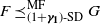
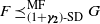




Remark 4. It is worth pointing out that for any non-decreasing functions
 $\boldsymbol{ \gamma}_1,\boldsymbol{ \gamma}_2\colon \mathbb{R} \rightarrow[0, 1]$
with
 $\boldsymbol{ \gamma}_1(t)\le \boldsymbol{ \gamma}_2(t)$
for every
 $t \in \mathbb{R}$
, we have
 \begin{equation*} \mathscr{U\,}^{\mathrm{MF}}_{\boldsymbol{ \gamma}_2} \, \subseteq \mathscr{U\,}^{\mathrm{MF}}_{\boldsymbol{ \gamma}_1} \quad \text{and} \quad \unicode{x1D4D4}_{\mathrm{MF}}(\boldsymbol{ \gamma}_2) \supseteq \unicode{x1D4D4}_{\mathrm{MF}}(\boldsymbol{ \gamma}_1).\end{equation*}
As mentioned earlier in Remark 1(iii), incorporating the function
 $\boldsymbol{ \gamma}$
as a CDF introduces an additional layer of randomness, enriching our framework. In line with this, we now present a probabilistic characterization of Proposition 5(c).
Proposition 6. Let
 $F,G,H_1,H_2$
be distribution functions such that
 $H_2 \preceq_{\mathrm{FSD}} H_1$
. Then relation
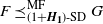 $F \preceq^{\mathrm{MF}}_{ (1+ \boldsymbol{H_1})\textrm{-SD}} G$
implies that
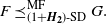 $F \preceq^{\mathrm{MF}}_{ (1+ \boldsymbol{H_2})\textrm{-SD}} G.$
Proposition 7. (Stability properties.) For an arbitrary non-decreasing function
 $\unicode{x1D6C4}$
, the multi-fractional
 $(1+\unicode{x1D6C4})$
-SD is closed under the following operations.
-
(a) Positive location transformations: for all
$c\ge 0$
,
\begin{equation*}X \preceq^{\mathrm{MF}}_{ (1+ \boldsymbol{ \gamma})\textrm{-SD}} Y \quad {implies\, that} \quad X+c \preceq^{\mathrm{MF}}_{ (1+ \boldsymbol{ \gamma})\textrm{-SD}} Y+c.\end{equation*}
-
(b) Convolutions with non-negative independent random variables:
where Z is non-negative and independent of X and Y.
\begin{equation*}X \preceq^{\mathrm{MF}}_{ (1+ \boldsymbol{ \gamma})\textrm{-SD}} Y \quad {implies\, that} \quad X+Z \preceq^{\mathrm{MF}}_{ (1+ \boldsymbol{ \gamma})\textrm{-SD}} Y+Z,\end{equation*}
-
(c) Mixing:
\begin{equation*}[X|\Theta=\theta]\preceq^{\mathrm{MF}}_{ (1+ \boldsymbol{ \gamma})\textrm{-SD}} [Y|\Theta=\theta], \quad {for\, all}\ \theta \in \operatorname{supp}(\Theta) \quad {implies\, that} \quad X \preceq^{\mathrm{MF}}_{ (1+ \boldsymbol{ \gamma})\textrm{-SD}} Y.\end{equation*}
-
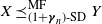
(d) Let
$(\boldsymbol{ \gamma}_n\colon n\ge 1)$
be a sequence of non-decreasing functions so that
$\unicode{x1D6C4}_n {\stackrel{\mathrm{p.wise}}{\longrightarrow}} \unicode{x1D6C4}$
as
$n \to \infty$
. Then
$\boldsymbol{ \gamma}$
is non-decreasing and, moreover, if
$X \preceq^{\mathrm{MF}}_{ (1+ \boldsymbol{ \gamma}_n)\textrm{-SD}} Y$
for every
$n \in \mathbb{N}$
, then
$X \preceq^{\mathrm{MF}}_{ (1+ \boldsymbol{ \gamma})\textrm{-SD}} Y$
.




Inspired by [Reference Müller, Scarsini, Tsetlin and Winkler23, Theorem 4.8], we provide the following result, which extends the invariance property to more general transformations.
Proposition 8. If
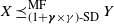 $X \preceq^{\mathrm{MF}}_{ (1+ \boldsymbol{ \gamma}\times\gamma)\textrm{-SD}} Y$
for a non-decreasing function
 $\boldsymbol{ \gamma}\colon \mathbb{R} \rightarrow[0, 1]$
and a constant
 $\gamma \in [0, 1]$
, then we have the following:
-
(a)
$ \phi(X) \preceq^{\mathrm{MF}}_{ (1+ \boldsymbol{ \gamma})\textrm{-SD}} \phi(Y)$
for all
$\phi \in \mathscr{U\,}^*_{\gamma}$
with
$\phi(x)\ge x$
, -
(b)
$\psi(X) \preceq_{ (1+ \gamma)\textrm{-SD}} \psi(Y)$
for all
$\psi \in \mathscr{U\,}^{\mathrm{MF}}_{\unicode{x1D6C4}}$
.





Remark 5. Recall that when
 $\gamma=1$
, the utility class
 $\mathscr{U\,}^*_\gamma$
consists of increasing concave functions. In the special case of Proposition 8 with
 $\gamma=1$
, it follows that (i) multi-fractional
 $(1+\unicode{x1D6C4})$
-SD is invariant under any increasing concave transformation
 $\phi$
satisfying
 $\phi(x) \ge x$
, and (ii) for every
 $\psi \in \mathscr{U\,}^{\mathrm{MF}}_{\unicode{x1D6C4}}$
, the relation
 $\psi(X) \preceq_{\mathrm{SSD}} \psi(Y)$
holds.
2.5. Connection with
$\gamma$
-transfers

In this section we briefly outline a connection to the notion of
 $\gamma$
-transfers introduced in [Reference Müller, Scarsini, Tsetlin and Winkler23]. In fact, the concept of restricted fractional
 $(1+\gamma)^r_t$
-SD, combined with Proposition 1, offers a natural route for formalizing this relationship. Following [Reference Müller, Scarsini, Tsetlin and Winkler23], for two discrete distributions F and G with probability mass functions f and g respectively, we say that:
-
(a) G is obtained from F via an increasing transfer if there exist
$x_1\! < x_2$
and
$\eta > 0$
such that
${g(x_1)} \, = \, {f(x_1)} - \eta$
,
${g(x_2)} \, = \, {f(x_2)} + \eta$
, and
$ {g(z)} \, = \,{ f(z)}$
for all other values of z, -
(b) G is obtained from F via a
$\gamma$
-transfer if there exist
$x_1\! < x_2 < x_3 < x_4$
and
$\eta_1, \eta_2 > 0$
with
$\eta_2(x_4 - x_3) = \gamma \eta_1 (x_2 - x_1)$
such that
${g(x_1)} \, = \, {f(x_1)} - \eta_1$
,
${g(x_2)} \, = \, {f(x_2)} + \eta_1$
,
${g(x_3)} \, = \, {f(x_3)} + \eta_2$
,
${g(x_4)} \, = \, {f(x_4)} - \eta_2$
, and
${g(z)} \, = \,{ f(z)}$
for all other values of z.














For notational convenience, for a given distribution F and
 $t \in \mathbb{R}$
, denote its right-censoring (or upper-tail truncation) version at level t by
 $F^r_t$
:
 \begin{equation*}F^r_t(x)\,:\!=\,\begin{cases}F(x), & x < t,\\1 , & x \ge t.\end{cases}\end{equation*}
Observe that if
 $X\sim F$
, then the right-censored random variable
 $X\wedge t \,:\!=\, \min\{X,t\}$
has distribution function
 $F_t^r$
. Now it follows immediately from Definition 3 that for fixed
 $t\in\mathbb{R}$
and
 $\gamma\in[0, 1]$
,
 \begin{equation*}F \preceq_{(1+\gamma)_{t}^r\textrm{-SD}} G\quad \Longleftrightarrow\quad F_t^r \preceq_{(1+\gamma)\textrm{-SD}} G_t^r .\end{equation*}
Next we can state the following proposition.
Proposition 9. (Multi-fractional SD and local
 $\unicode{x1D6C4}(t)$
-transfers.) Let F and G be distribution functions on
 $\mathbb{R}$
with finite means, and consider an arbitrary non-decreasing function
 $\unicode{x1D6C4}\colon \mathbb{R}\to[0, 1]$
. Assume
 $X\sim F$
and
 $Y\sim G$
. Then the following statements are equivalent:
-
(a)
$F \preceq^{\mathrm{MF}}_{(1+\unicode{x1D6C4})\textrm{-SD}} G$
, -
(b)
$F^r_t \preceq_{(1+\unicode{x1D6C4} (t))\textrm{-SD}} G^r_t$
for every t, -
(c) for every t, there exist two sequences
$\{X_n^{(t)}\}_{n\in\mathbb{N}}$
and
$\{Y_n^{(t)}\}_{n\in\mathbb{N}}$
such that, for all
$n\in \mathbb{N}$
, the distribution of
$Y^{(t)}_n$
can be obtained from the distribution of
$X^{(t)}_n$
via a finite sequence of
$\unicode{x1D6C4}(t)$
-transfers and increasing transfers, and as n tends to infinity, we have
\begin{equation*}X_n^{(t)} \stackrel{\text{law}}{\Longrightarrow} X\wedge t \quad {and} \quad Y_n^{(t)} \stackrel{\text{law}}{\Longrightarrow} Y\wedge t.\end{equation*}




Remark 6. In particular, when the function
 $\unicode{x1D6C4}$
is piecewise constant with finitely many jumps, the set of transfer parameters
 $\{\unicode{x1D6C4}(t)\colon t\in\mathbb{R}\}$
is finite. Hence, across all censoring levels t, the MFSD relation can be characterized using only finitely many types of
 $\unicode{x1D6C4}(t)$
-transfer operations (together with increasing transfers). For a general
 $\unicode{x1D6C4}$
, one can find a sequence
 $(\unicode{x1D6C4}_n)_{n\ge1}$
of non-decreasing, right-continuous, piecewise constant functions with finitely many jumps such that
 $\unicode{x1D6C4}_n \uparrow \unicode{x1D6C4}$
pointwise, and observe that if
 $F \preceq_{(1+\unicode{x1D6C4}_n(t))_{t}^r\textrm{-SD}} G$
holds for every n, then Proposition 7(d) yields
 $F \preceq_{(1+\unicode{x1D6C4}(t))_{t}^r\textrm{-SD}} G$
.
3. Generalization through utility class
In this section we study a generalization of fractional
 $(1+\gamma)$
-SD via the utility class in (2), which gives rise to generalized families of functional fractional stochastic dominance (FFSD).
3.1. FFSD: Definition and the integral condition
In Section 2 we extended fractional
 $(1+\gamma)$
-SD using an integral condition by replacing the constant parameter
 $\gamma$
with its functional analogue
 $\unicode{x1D6C4}$
. Due to the nature of the integral condition (1), this extension was relatively straightforward, as it involves associating the function
 $\unicode{x1D6C4}$
with a single point. However, the extension via the utility class introduces additional complexity, since the set condition for
 $\mathscr{U\,}^{*}_{\gamma}$
given in (2) involves four points. Therefore we require a new framework that enables a functional extension using a function
 $\unicode{x1D6C4}$
of a single variable. We construct this framework with the following requirements in mind.
-
(i) Fractional SD should be representable such that, for any
$\gamma \in [0, 1]$
, the set condition given in (2) is both necessary and sufficient to verify whether a given function u belongs to the fractional SD utility space within the new framework (see Proposition 10). -
(ii) The framework must be meaningful for decision analysis (see Section 4).

Based on the discussion above, we build our framework using the one-sided derivatives of utility functions. This approach not only serves our purposes but also provides a tractable and meaningful structure. Hence we introduce the following.
Definition 5. We say that a function u has the
 ${\boldsymbol{{D}}}_{\pm}$
property if u is two-sided differentiable, that is, the left-derivative
 $ u_-'(x) $
and the right-derivative
 $ u_+'(x) $
exist at each point
 $ x \in \mathbb{R}$
. For a given
 $\gamma \in [0, 1]$
, we define
 \begin{equation*}\widetilde{\mathscr{U\,}}^{*}_{\gamma} \,:\!=\, \mathscr{U\,}^{*}_{\gamma} \cap \mathscr{U\,}({\boldsymbol{{D}}}_{\pm}),\end{equation*}
where
 \begin{equation*} \mathscr{U\,}({\boldsymbol{{D}}}_{\pm})\,:\!=\, \{ u \colon \mathbb{R} \to \mathbb{R} \colon \textit{u}\text{ satisfies the $ {\boldsymbol{{D}}}_{\pm} $ property} \}.\end{equation*}
We present the following proposition, which establishes the representability of fractional SD.
Proposition 10. Let u be a function whose left- and right-derivatives exist at each point
 $x \in \mathbb{R}$
. Then, for a given
 $\gamma \in [0, 1]$
, we have
 $u\in \widetilde{\mathscr{U\,}}^{*}_{\gamma}$
if and only if
 \begin{equation*}0\le\gamma u_+'(y) \le u_+'(x)\quad \textit{for all $ x \le y$.}\end{equation*}
A similar conclusion holds for the left-derivative
 $u'_-$
.
Building on our development so far, we provide the following derivative-relation property for the functional extension of
 $\widetilde{\mathscr{U\,}}^{*}_{\gamma}$
.
Definition 6. (
 ${\boldsymbol{{D}}}_{\pm}(\unicode{x1D6C4})$
-property.) Let
 $\unicode{x1D6C4}\colon \mathbb{R}\to[0, 1]$
be an arbitrary non-decreasing function. We say that a function
 $u\colon \mathbb{R} \to \mathbb{R}$
satisfies the
 ${\boldsymbol{{D}}}_{\pm}(\unicode{x1D6C4})$
-property if it is differentiable from both sides (i.e. it has the
 ${\boldsymbol{{D}}}_{\pm}$
property) and, moreover, at least one of the following conditions hold:
 \begin{equation}{\rm (i)} \quad 0 \le \unicode{x1D6C4} (y) u_+'(y) \le u_+'(x) \quad \text{for all $x \le y$,}\quad {\rm (ii)} \quad 0 \le \unicode{x1D6C4}(y) u'_-(y) \le u'_{-}(x) \quad \text{for all $ x\le y$.}\end{equation}
Clearly, conditions (i) and (ii) are equivalent and simplify, at points where u is differentiable, to
 $0 \le \unicode{x1D6C4}(y)\,u'(y) \le u'(x)$
for all
 $ x \le y$
. We will revisit this relationship in Proposition 13. For a given non-decreasing function
 $\unicode{x1D6C4}\colon \mathbb{R}\to[0, 1]$
, we define the following utility space:
 \begin{equation*} \widetilde{\mathscr{U\,}}^{\mathrm{FF}}_{\unicode{x1D6C4}}\,:\!=\, \{ u\colon \mathbb{R} \to \mathbb{R} \colon \textit{u} \text{ satisfies the $ {\boldsymbol{{D}}}_{\pm(\unicode{x1D6C4})}$-property} \}.\end{equation*}
Now we are ready to define functional fractional stochastic dominance.
Definition 7. (Functional fractional
 $(\boldsymbol{ \gamma})$
-SD.) Let
 $\unicode{x1D6C4}\colon \mathbb{R} \to [0, 1]$
be an arbitrary non-decreasing function, and let F and G be two distribution functions. We say that G dominates F in the sense of functional fractional
 $(\unicode{x1D6C4})$
-SD, denoted by
 $F \preceq^{\mathrm{FF}}_{\unicode{x1D6C4}\textrm{-SD}} G$
, if
 \begin{equation*} \mathbb{E}_F[u] \le \mathbb{E}_G[u] \quad \text{for all $ u \in \widetilde{\mathscr{U\,}}^{\mathrm{FF}}_{\unicode{x1D6C4}}$,}\end{equation*}
provided that the expectations exist.
The following result establishes the relationship between MFSD and FFSD.
Proposition 11. Let
 $\boldsymbol{ \gamma}\colon \mathbb{R} \to [0, 1]$
be an arbitrary non-decreasing function. Then the inclusion
 $ \widetilde{\mathscr{U\,}}^{\mathrm{MF}}_{\unicode{x1D6C4}} \subseteq \widetilde{\mathscr{U\,}}^{\mathrm{FF}}_{\unicode{x1D6C4}} $
holds. Moreover, if
 $\unicode{x1D6C4}\equiv \gamma\in [0, 1]$
, the two sets coincide.
Remark 7.
-
(i) When transitioning from a fixed coefficient
$\gamma$
to its functional form
$\unicode{x1D6C4}$
, the utility space
$\widetilde{\mathscr{U\,}}^{\mathrm{FF}}_{\unicode{x1D6C4}}$
emerges as a natural generalization of
$\widetilde{\mathscr{U\,}}^*_{\gamma}$
. This resembles the extension observed in the MFSD framework, where the integral condition is adapted to incorporate the functional form of
$\boldsymbol{ \gamma}$
. A closer examination of the
${\boldsymbol{{D}}}_{\pm}(\unicode{x1D6C4})$
-property reveals that
$\unicode{x1D6C4}$
controls the maximal possible increase in the one-sided derivatives based on location, i.e.
$u_+(y)/u_+(x) \le 1/\unicode{x1D6C4}(y)$
, where its non-decreasing nature permits a greater increase at lower values on the real line. This implies that steeper local convexities are allowed at lower values. Although
$\boldsymbol{ \gamma}$
has similar interpretations in the class
$\widetilde{\mathscr{U\,}}^{\mathrm{MF}}_{\unicode{x1D6C4}}$
, its control in
$\widetilde{\mathscr{U\,}}^{\mathrm{FF}}_{\unicode{x1D6C4}}$
is more localized, permitting utility functions to be more non-concave. In fact, as discussed in Remark 11, we can construct an insightful example of such a function for which
$u \in \widetilde{\mathscr{U\,}}^{\mathrm{FF}}_{\unicode{x1D6C4}}$
but
$u \notin \widetilde{\mathscr{U\,}}^{\mathrm{MF}}_{\unicode{x1D6C4}}$
. In general, we have
$\widetilde{\mathscr{U\,}}^{\mathrm{FF}}_{\unicode{x1D6C4}}\setminus \widetilde{\mathscr{U\,}}^{\mathrm{MF}}_{\unicode{x1D6C4}}\neq \emptyset$
as soon as
$\boldsymbol{ \gamma}\not\equiv \gamma$
for some
$\gamma \in [0, 1]$
. -
(ii) One advantage of the utility class
$\widetilde{\mathscr{U\,}}^{\mathrm{FF}}_{\unicode{x1D6C4}}$
is that, for a given utility function u, determining whether
$u \in \widetilde{\mathscr{U\,}}^{\mathrm{FF}}_{\unicode{x1D6C4}}$
is relatively straightforward compared to checking membership in
$\widetilde{\mathscr{U\,}}^{\mathrm{MF}}_{\unicode{x1D6C4}}$
. The inclusion relation in Proposition 11 allows us to develop tools that can easily determine whether a given function
$u \in \widetilde{\mathscr{U\,}}^{\mathrm{FF}}_{\unicode{x1D6C4}}$
also belongs to
$\widetilde{\mathscr{U\,}}^{\mathrm{MF}}_{\unicode{x1D6C4}}$
. In Section 4 we introduce the notion of partial greediness, which not only provides meaningful decision-theoretic interpretations but also facilitates this verification. -
(iii) The bounds on the upward jumps in the derivative
$u^{\prime}$
at kink points depend on the location of the kink. For example, let
$x^*_1<x^*_2$
be two points at which u has kinks. Then Such a feature is not available in the context of
\begin{equation*}\dfrac{u_+^{\prime}(x^*_1)}{u_-^{\prime}(x^*_1)} \le \dfrac{1}{\boldsymbol{ \gamma}(x^*_1) } \quad \text{and} \quad \dfrac{u_+^{\prime}(x^*_2)}{u_-^{\prime}(x^*_2)} \le \dfrac{1}{\boldsymbol{ \gamma}(x^*_2)}.\end{equation*}
$\widetilde{\mathscr{U\,}}^*_\gamma$
, where the ratio
$1/\gamma$
provides a global bound that is independent of the locations of the kinks.





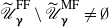


Next, we prove an ‘if and only if’ theorem for FFSD that establishes a connection with the integral condition:
 \begin{equation}\int_{-\infty}^t \dfrac{1}{\boldsymbol{ \gamma}(x)}(F(x)-G(x))_- \,{\mathrm{d}} x \le \int_{-\infty}^t (F(x)-G(x))_+ \,{\mathrm{d}} x \quad \text{for all $t \in \mathbb{R}$.}\end{equation}
But first we make the following remark concerning the well-definedness of the integral condition.
Remark 8. For a given function
 $\unicode{x1D6C4}$
and distribution functions F and G, the integral condition (8) is well-defined if the integral on the left-hand side is finite for every
 $t \in \mathbb{R}$
. First,
 $(F(x)-G(x))_-$
is bounded and non-negative, and assuming
 $\unicode{x1D6C4}\colon \mathbb{R} \to (0,1]$
, ensures that
 ${{1}/{(\unicode{x1D6C4}(x))}}$
is well-defined. Moreover, we impose the following assumptions:
-
(i) the distribution functions have finite means,
-
(ii) the first crossing point between the distributions,
$x_1^*$
, exists, and
$(F(x)-G(x))_- = 0$
for all
$x \le x_1^*$
.



If the distributions never cross, then (8) holds trivially, and the statements follow directly from FSD. Therefore, for a given non-decreasing function
 $\unicode{x1D6C4}\colon \mathbb{R} \to (0,1]$
, by the monotonicity of
 $\unicode{x1D6C4}$
we have
 \[\int_{-\infty}^{t}\dfrac{1}{\unicode{x1D6C4}(x)}(F(x)-G(x))_- \,{\mathrm{d}} x\le\int_{x^*_1}^{t}\dfrac{1}{\unicode{x1D6C4}(x^*_1)}(F(x)-G(x))_-\,{\mathrm{d}} x\quad \text{for all $ t \in \mathbb{R}$.}\]
Now we begin by establishing one direction of the ‘if and only if’ theorem.
Lemma 2. Let
 $\boldsymbol{ \gamma}\colon \mathbb{R} \rightarrow (0,1]$
be an arbitrary non-decreasing right-continuous function with finitely many jumps. Let F and G be two arbitrary distribution functions crossing finitely many times. For every
 $t \in \mathbb{R}$
, define the continuous function
 $u_{\mathrm{FF},t}$
via its right-derivative as
 \begin{equation*} u_{\mathrm{FF},t}^{\prime}(x)=\begin{cases}1 & {if \, G(x) \le F(x)\, and \, x \leq t\,,} \\1/\boldsymbol{ \gamma}(x) & {if \, F(x) < G(x)\, and \, x \leq t\,,} \\0 & {if \, t < x\,.}\end{cases}\end{equation*}
Then
 $u_{\mathrm{FF},t} \in\widetilde{\mathscr{U\,}}^{\mathrm{FF}}_{\unicode{x1D6C4}}$
for every
 $t \in \mathbb{R}$
.
Proposition 12. Let
 $\boldsymbol{ \gamma}\colon \mathbb{R} \rightarrow (0,1]$
be an arbitrary non-decreasing right-continuous function with finitely many jumps. Let F and G be two arbitrary distribution functions with finite means and crossing finitely many times. Then the relation
 \begin{equation*} \mathbb{E}_F[u_{\mathrm{FF},t}] \le \mathbb{E}_G [u_{\mathrm{FF},t}] \quad {for\, all \, t \in \mathbb{R}}\end{equation*}
implies that the integral condition (8) holds.
We are now prepared to present the main theorem.
Theorem 3. Let
 $ \unicode{x1D6C4}\colon \mathbb{R} \to (0,1] $
be a non-decreasing, right-continuous function with a finite number of discontinuities. Consider two distribution functions F and G that intersect only finitely many times. Then the following statements are equivalent:
-
(a)
$ F \preceq^{\mathrm{FF}}_{\unicode{x1D6C4}\textrm{-SD}} G $
, -
(b) the integral condition (8) holds, that is,
\begin{equation*}\int_{-\infty}^t \dfrac{1}{\boldsymbol{ \gamma}(x)}(F(x)-G(x))_- \,{\mathrm{d}} x \le \int_{-\infty}^t (F(x)-G(x))_+ \,{\mathrm{d}} x \quad {for\, all \,t \in \mathbb{R}.}\end{equation*}


Remark 9. The integral condition (8) admits a geometric interpretation as a balance of areas at every threshold t: positive gaps are integrated with respect to the Lebesgue measure
 ${\mathrm{d}} x$
, whereas negative gaps are effectively reweighted by the location-dependent factor
 ${\mathrm{d}} x/\unicode{x1D6C4}(x)$
. In view of the local
 $\unicode{x1D6C4}(t)$
-transfer interpretation of MFSD (Proposition 9), this motivates a transfer-based perspective for FFSD. Let
 $\unicode{x1D6C4}\colon \mathbb{R}\to(0,1]$
be a non-decreasing function. Fix
 $x_1\! < x_2\le x_3 < x_4$
and let
 $\eta_1,\eta_2>0$
. A
 $\unicode{x1D6C4}$
-weighted transfer consists of moving probability mass
 $\eta_1$
from
 $x_1$
to
 $x_2$
and simultaneously moving probability mass
 $\eta_2$
from
 $x_4$
to
 $x_3$
, subject to the balance constraint
 \[\eta_2\int_{x_3}^{x_4}\dfrac{{\mathrm{d}} x}{\unicode{x1D6C4}(x)}=\eta_1\,(x_2-x_1).\]
Such weighted transfers, together with increasing transfers in the sense of [Reference Müller, Scarsini, Tsetlin and Winkler23], preserve the FFSD integral condition (8) uniformly over all censoring thresholds t. Under the regularity conditions of Theorem 3, one could potentially further develop an FFSD analogue of Proposition 9; however, we do not pursue these technical details here.
We conclude this section with the following remark.
Remark 10.
-
(i) As established in Proposition 11, functional fractional stochastic dominance (FFSD) is stronger than MFSD, and therefore implies SSD. Moreover, FSD implies FFSD. Hence
If
\begin{equation*}\mathrm{FSD} \quad \Longrightarrow \quad \mathrm{FFSD} \quad \Longrightarrow \quad \mathrm{MFSD} \quad \Longrightarrow \quad \mathrm{SSD}.\end{equation*}
$\unicode{x1D6C4}\equiv \gamma \in (0,1]$
is constant, then FFSD reduces to MFSD. At the endpoint
$\gamma=1$
, we re-cover SSD. In the limit as
$\gamma\to 0$
, we recover FSD, since this forces
$(F(x)-G(x))_- \equiv 0$
on
$\mathbb{R}$
. Moreover, the integral condition (8) is monotone in
$\boldsymbol{ \gamma}$
, and hence we have the sandwich of orders
\begin{equation*}F \preceq^{\mathrm{FF}}_{{\!\substack{{\unicode{x1D6C4}}\\\rule{.6em}{1.5pt}}}\textrm{-SD}} G \quad \Longrightarrow \quad F \preceq^{\mathrm{FF}}_{\unicode{x1D6C4}\textrm{-SD}} G \quad \Longrightarrow \quad F \preceq^{\mathrm{FF}}_{\stackrel{\rule{.6em}{1.4pt}}{\unicode{x1D6C4}}\textrm{-SD}} G.\end{equation*}
-
(ii) Following Proposition 11, it is evident that
$ \widetilde{\mathscr{U\,}}^*_{\stackrel{\rule{.6em}{1.5pt}}{\unicode{x1D6C4}}} \subseteq \widetilde{\mathscr{U\,}}^{\mathrm{MF}}_{\unicode{x1D6C4}} \subseteq \widetilde{\mathscr{U\,}}^{\mathrm{FF}}_{\unicode{x1D6C4}} \subseteq \widetilde{\mathscr{U\,}}^{*}_{\!\substack{{\unicode{x1D6C4}}\\\rule{.6em}{1.5pt}}}$
and these inclusions are strict as soon as
$ \unicode{x1D6C4} $
is a non-constant function. In the terminology of Section 2.2, the inclusion relation
$ \unicode{x1D4D4}_{\mathrm{FF}}(\unicode{x1D6C4}) \subseteq \unicode{x1D4D4}_{\mathrm{MF}} (\unicode{x1D6C4})$
for the universe of distributions is directly verified by the integral conditions (3) and (8). -
(iii) There is a particularly interesting aspect here that is worth highlighting. Both MFSD and FFSD interpolate between FSD and SSD, but they do so in distinct ways. MFSD, via its integral condition (3), provides a form of local interpolation that is easy to interpret. However, when we consider the corresponding utility class
$ \mathscr{U\,}^{\mathrm{MF}}_{\unicode{x1D6C4}} $
, the interpolation is less transparent: it is difficult both to interpret and to verify whether a given utility function belongs to this class. In contrast, for FFSD the interpolation is clearly visible in the utility class
$ \widetilde{\mathscr{U\,}}^{\mathrm{FF}}_{\unicode{x1D6C4}} $
, which allows for easy verification of whether a given utility function belongs to it. However, the integral condition (8) lacks a clear interpretation of how FFSD interpolates between FSD and SSD, unlike in MFSD.










3.2. FFSD: Examples
In this section we present examples that highlight the key differences between the MFSD and FFSD frameworks. Given the inclusion
 $\widetilde{\mathscr{U\,}}^{\mathrm{MF}}_{\unicode{x1D6C4}} \subseteq \widetilde{\mathscr{U\,}}^{\mathrm{FF}}_{\unicode{x1D6C4}}$
given in Proposition 11, it follows that all example utility functions presented in Section 2.3 for
 $\mathscr{U\,}^{\mathrm{MF}}_{\unicode{x1D6C4}}$
also belong to
 $\widetilde{\mathscr{U\,}}^{\mathrm{FF}}_{\unicode{x1D6C4}}$
, provided they are two-sided differentiable. There are also non-differentiable functions outside the MFSD utility class, but we focus on those that are both realistic and practically significant. Specifically, we concentrate on the family of piecewise continuously differentiable (PCD) functions, which are particularly relevant for modelling decision-making behaviour in applications.
Proposition 13. Let
 $u\colon \mathbb{R}\to \mathbb{R}$
be a piecewise continuously differentiable function. Then the following hold.
-
(a) u is two-sided differentiable on
$\mathbb{R}$
, that is, it satisfies the
${\boldsymbol{{D}}}_{\pm}$
property. -
(b) Let
$\unicode{x1D6C4}\colon \mathbb{R}\to[0, 1]$
be a non-decreasing function that is continuous at each subdivision point
$\{x_1,\dots,x_n\}$
of u. Then the following two derivative conditions are equivalent:
\begin{alignat*}{3}&{\rm (i)} &\quad 0 &\le \unicode{x1D6C4}(y)\,u'_+(y) \le u'_+(x)\quad {for\, all\, x \le y,} \\&{\rm (ii)} &\quad 0 &\le \unicode{x1D6C4}(y)\,u'_-(y) \le u'_-(x)\quad {for\, all \, x \le y.}\end{alignat*}


Proposition 13(a) establishes that PCD functions indeed belong to
 $\widetilde{\mathscr{U\,}}^{\mathrm{FF}}_{\unicode{x1D6C4}}$
provided that they satisfy the derivative-relation property for an appropriately chosen function
 $\unicode{x1D6C4}$
. It is also possible to use mixed-side conditions, such as
 \[0 \le \unicode{x1D6C4}(y) u'_+(y) \le u'_-(x)\quad \text{for all $ x\le y$.}\]
This condition is particularly useful in scenarios where the utility function exhibits upward jumps in its derivative, as discussed in Remark 7(iii). On the other hand, PCD functions are not necessarily included in
 $\widetilde{\mathscr{U\,}}^{\mathrm{MF}}_{\unicode{x1D6C4}}$
, since its definition requires u to be expressible as a linear combination of functions in
 $\widetilde{\mathscr{U\,}}^{\mathrm{Union}}_{\unicode{x1D6C4}}$
. To illustrate this distinction further, we provide the FFSD counterpart of Example 6. This example also highlights key structural differences between
 $\widetilde{\mathscr{U\,}}^{\mathrm{FF}}_{\unicode{x1D6C4}}$
and
 $\widetilde{\mathscr{U\,}}^*_{\gamma}$
.
Example 7. The purpose of this example is to provide a parametrized family
 $\mathscr{U\,}_{\Theta}$
such that the inclusion
 $\mathscr{U\,}_{\Theta} \subseteq \widetilde{\mathscr{U\,}}^*_{\gamma}$
can hold for a constant
 $\gamma \in [0, 1]$
only if
 $\gamma=0$
(hence corresponding to the utility class for FSD). However, one can choose a suitable non-decreasing function
 $\unicode{x1D6C4}$
such that
 \begin{equation*}\mathscr{U\,}_{\Theta} \subseteq \widetilde{\mathscr{U\,}}^{\mathrm{FF}}_{\unicode{x1D6C4}} \neq \widetilde{\mathscr{U\,}}_{0} \quad \text{and more importantly} \quad \mathscr{U\,}_{\Theta} \not\subseteq \widetilde{\mathscr{U\,}}^{\mathrm{MF}}_{\unicode{x1D6C4}}.\end{equation*}
Let
 $\Theta=(0,1)$
and consider a function
 $\widetilde{\unicode{x1D6C4}} \colon \Theta \to (0,1)$
with
 $\lim_{\theta \to 0}\widetilde{\unicode{x1D6C4}}(\theta)=0$
. For every
 $\theta \in \Theta$
, we define the following PCD utility function
 $u_\theta$
via its right-derivative as
 \begin{equation*}u'_\theta(x)=\begin{cases}u_{\theta,1}^{\prime}(x) & \text{if $ -\infty< x < \theta$,}\\x & \text{if $ \theta\le x < \sqrt{\theta} $,}\\u_{\theta,2}^{\prime}(x) & \text{if $ \sqrt{\theta}\le x < \infty$,}\\\end{cases}\end{equation*}
where
 $u_{\theta,1}^{\prime}$
and
 $u_{\theta,2}^{\prime}$
are arbitrary non-negative and non-increasing continuous functions with
 $\inf_{x\in \mathbb{R}}u_{\theta,1}^{\prime}(x)=\sqrt{\theta}$
and
 $\sup_{x\in \mathbb{R}} u_{\theta,2}^{\prime}(x)=\theta$
. Thus, for a given
 $\theta$
, it is straightforward to see that
 $u_\theta \in \widetilde{\mathscr{U\,}}^{*}_{\gamma}$
for some constant
 $\gamma$
(i.e. we have
 $ 0 \le \gamma u'_{\theta}(y) \le u'_{\theta} (x)$
for all
 $ x\le y $
) if and only if the condition
 \begin{equation}\sqrt{\theta} \ge \gamma\end{equation}
holds true. Let
 $\mathscr{U\,}_{\Theta } \,:\!=\, \{ u_\theta \colon \theta \in \Theta \}$
. Now observe that, for some constant
 $\gamma$
, the validity of the set inclusion
 $\mathscr{U\,}_{\Theta} \subseteq \mathscr{U\,}^*_{\gamma}$
dictates that necessarily
 $\gamma=0$
. This conclusion directly follows from (9) when
 $\theta\to 0$
. Hence the only scenario where
 $u_\theta$
for every
 $\theta\in \Theta$
included within a single utility space associated with the fractional
 $(1+\gamma)$
-SD corresponds to the utility class
 $\widetilde{\mathscr{U\,}}_{0} = \widetilde{\mathscr{U\,}}^*_{\gamma=0}$
. Next, consider the continuous non-decreasing function
 \begin{align*}\boldsymbol{ \gamma} (x) =\begin{cases}0 & \text{if $ x < 0 $,}\\x &\text{if $ 0 \le x \le 1$,}\\1 & \text{if $ x >1$.}\end{cases}\end{align*}
We first show that
 $\mathscr{U\,}_{\Theta} \subseteq \widetilde{\mathscr{U\,}}^{\mathrm{FF}}_{\unicode{x1D6C4}}$
. In order to do this, note that, for each
 $\theta \in \Theta$
, the condition
 \begin{equation}\theta \ge u'_{\theta}(y) \boldsymbol{ \gamma}(y) = y \times y \quad \text{for all $y \in [\theta, \sqrt{\theta})$}\end{equation}
is both necessary and sufficient for the validity of
 $u_\theta \in \widetilde{\mathscr{U\,}}^{\mathrm{FF}}_{\unicode{x1D6C4}}$
, which obviously holds true. Lastly, we show that
 $\mathscr{U\,}_{\Theta} \not\subseteq \widetilde{\mathscr{U\,}}^{\mathrm{MF}}_{\unicode{x1D6C4}}$
. Fix
 $\theta \in \Theta$
. First, when
 $y\approx\sqrt{\theta}$
(from left) and
 $x=\theta< y$
, it follows from (10) that
 \begin{equation}\dfrac{1}{\boldsymbol{ \gamma}(y)}=\dfrac{1}{\sqrt{\theta}}=\dfrac{u_\theta'(y)}{u_\theta'(x)}.\end{equation}
Next, we discuss that
 $u_\theta \notin \widetilde{\mathscr{U\,}}^{\mathrm{Union}}_{\unicode{x1D6C4}}$
. Note that
 $u_\theta$
is not a globally concave function and hence
 $u_\theta \notin \widetilde{\mathscr{U\,}}^{+\infty}_{{\stackrel{\rule{.6em}{1.5pt}}{\unicode{x1D6C4}}} =1}$
. Now, by contradiction, assume that there exists
 $t\in \mathbb{R} $
such that
 $u_\theta \in \widetilde{\mathscr{U\,}}^t_{\unicode{x1D6C4}(t)}$
. Therefore, based on the equality in (11), this is only possible when
 $t=\sqrt{\theta}$
. However, this leads to a contradiction, as the derivative of the subsequent concave segment,
 $u'_{2,\theta}$
of
 $u_\theta$
is not necessarily equal to 0 after
 $\sqrt{\theta}$
. Hence
 $u_\theta$
can only belong to
 $ \widetilde{\mathscr{U\,}}^{\mathrm{MF}}_{\unicode{x1D6C4}}$
if it can be represented as a convex combination of functions that belong to
 $\widetilde{\mathscr{U\,}}^{\mathrm{Union}}_{\unicode{x1D6C4}}$
. For the moment, assume that
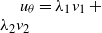 $u_\theta = \lambda_1 v_1 + \lambda_2 v_2$
where
 $v_1 \in \widetilde{\mathscr{U\,}}^{t = \sqrt{\theta}}_{\unicode{x1D6C4}(t) =\sqrt{\theta}}$
with
 ${{v_1'(\sqrt{\theta})}/{v_2'(\theta)}}={{1}/{\sqrt{\theta}}}$
and
 $v_2 \in \widetilde{\mathscr{U\,}}^*_{1}$
. Then, from the mediant inequality, we obtain
 \begin{equation*}\dfrac{u_\theta'(\sqrt{\theta})}{u_\theta'(\theta)}=\dfrac{\lambda_1v_1(\sqrt{\theta})+\lambda_2v_2(\sqrt{\theta})}{\lambda_1v_1(\theta)+\lambda_2v_2(\theta)}=\dfrac{\lambda_1\sqrt{\theta}+\lambda_2v_2(\sqrt{\theta})}{\lambda_1\theta+\lambda_2v_2(\theta)}<\dfrac{1}{\sqrt{\theta}}\end{equation*}
since
 ${{v_2(\sqrt{\theta})}/{v_2(\theta)}}\le 1$
for any
 $v_2\in \widetilde{\mathscr{U\,}}^*_{1}$
by definition, which violates (11). The general case can be discussed in a similar way relying on mediant inequality and the fact that any linear combination should contain at least one piece from the utility space
 $\widetilde{\mathscr{U\,}}^{\sqrt{\theta}}_{\sqrt{\theta}}$
and another piece from
 $\widetilde{\mathscr{U\,}}^{*}_{1}$
.
Plot of
 $u_\theta'$
.

We conclude with the following remark.
Remark 11. In addition to the examples above, we can also construct a non-decreasing function
 $\unicode{x1D6C4}$
and a utility function
 $u \in \widetilde{\mathscr{U\,}}^{\mathrm{FF}}_{\unicode{x1D6C4}}$
such that
 $u \notin \widetilde{\mathscr{U\,}}^{\mathrm{MF}}_{\unicode{x1D6C4}}$
. Moreover, there exist distribution functions F and G with
 $F \preceq^{\mathrm{MF}}_{(1+\unicode{x1D6C4})\textrm{-SD}} G$
such that the constructed function u violates the non-negativity condition
 $\mathbb{E}_G[u] - \mathbb{E}_F[u] \geq 0$
. While the construction of these functions and distributions is straightforward, it is omitted here for brevity (see [Reference Hür11, Example 4.2.2.]). This confirms that the class
 $\widetilde{\mathscr{U\,}}^{\mathrm{FF}}_{\unicode{x1D6C4}}$
cannot serve as a utility class for MFSD, contrary to what one might naturally expect.
4. MFSD and FFSD: Economic aspects
In this section we focus on examining the decision-theoretic aspects of both the FFSD and MFSD frameworks. In addition, we introduce a novel concept of partial greediness, which not only offers insights from an economic perspective but also provides a straightforward criterion for determining whether a given utility function in
 $\widetilde{\mathscr{U\,}}^{\mathrm{FF}}_{\unicode{x1D6C4}}$
is also contained in
 $\widetilde{\mathscr{U\,}}^{\mathrm{MF}}_{\unicode{x1D6C4}}$
.
4.1. Partial greediness
We introduce the novel notion of partial greediness of a utility function at an arbitrary point
 $x\in \mathbb{R}$
that provides a meaning to the function
 $\boldsymbol{ \gamma}$
from a decision-making perspective in both the multi-fractional and functional fractional stochastic dominance frameworks. The notion of partial greediness at the location
 $x\in \mathbb{R}$
characterizes the greediness behaviour of decision makers over half-open intervals
 $(x,\infty)$
, rather than over the entire real line, as in [Reference Chateauneuf, Cohen and Meilijson5]. They define the index of global greediness (non-concavity) for a strictly increasing function
 $u\colon \mathbb{R}\to \mathbb{R}$
as follows:
 \begin{equation}G_u\,:\!=\, \sup\nolimits _{x_1 < x_2 \leq x_3 < x_4}\biggl(\dfrac{u(x_4)-u(x_3)}{x_4-x_3} \bigg/ \dfrac{u(x_2)-u(x_1)}{x_2-x_1}\biggr).\end{equation}
It is known that always
 $G_u \ge 1$
and
 $G_u =1$
if and only if u is a concave function. Moreover, when u is differentiable, it is true that
 $G_u = \sup_{x \le y} u'(y)/ u'(x)$
(see [Reference Chateauneuf, Cohen and Meilijson5]). In this regard, the index
 $G_u$
globally determines the maximal magnitude of the increase in the slope of the utility function (marginal utility) over its entire domain. Upon closer examination of the set condition of the utility space
 $\mathscr{U\,}^*_{\gamma}$
, as provided in (2), it becomes evident that
 $\gamma$
serves as an upper bound for the level of greediness (non-concavity)
 $G_u$
for all
 $u \in \mathscr{U\,}^*_\gamma$
, established by the inequality
 $G_u \leq 1/\gamma$
. Inspired by [Reference Chateauneuf, Cohen and Meilijson5], we define a more local version of the greediness index as follows.
Definition 8. (Discrete partial greediness.) Let u be a strictly increasing function. The discrete partial greediness at location
 $x \in \mathbb{R}$
is defined as
 \begin{equation*} G^d_{\mathrm{par}}(u;\,x)\,:\!=\, \sup\nolimits_{x < x_1 < x_2\le x_3 < x_4}\biggl(\dfrac{u(x_4)-u(x_3)}{x_4-x_3}\bigg/\dfrac{u(x_2)-u(x_1)}{x_2-x_1}\biggr).\end{equation*}
Proposition 14.
-
(a) Clearly
$G^d_{\mathrm{par}}(u;\cdot) \le G_u$
, where the global index of greediness
$G_u$
is given by (12). -
(b) The function
$x \mapsto G^d_{\mathrm{par}}(u;\,x)$
is non-increasing, i.e.
$G^d_{\mathrm{par}}(u;\,x_2) \le G^d_{\mathrm{par}}(u;\,x_1)$
for
$x_1 \le x_2$
. Moreover,
$G^d_{\mathrm{par}}(u;\,x) \to G_u$
as
$x \to -\infty$
. -
(c) For every x,
$G^d_{\mathrm{par}}(u;\,x) \ge 1$
and
$G^d_{\mathrm{par}}(u;\,x)=1$
if and only if u is concave on
$(x,\infty)$
. In addition, u is concave on
$\mathbb{R}$
if and only if
$G^d_{\mathrm{par}}(u;\,x)=1$
for every
$x\in\mathbb{R}$
. -
(d) The function
$x \mapsto G^d_{\mathrm{par}}(u;\,x)$
is right-continuous.
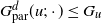




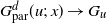


Remark 12.
-
(i) From a mathematical perspective,
$G^d_{\mathrm{par}}(u;\,x)$
is a measure of non-concavity over half-open intervals
$(x, \infty)$
. -
(ii) In the context of decision theory,
$G_u$
serves as a global measure, capturing the maximal proportional increase in a decision-maker’s valuation of an additional cent as wealth transitions from lower to higher values. Thus
$G_u$
takes into account all possible wealth levels, making it a natural measure of global greediness over
$\mathbb{R}$
. Building on the concept of
$G_u$
, for a fixed wealth level
$x\in \mathbb{R}$
, the measure
$G^d_{\mathrm{par}}(u;\,x)$
provides a region-restricted analogue of global greediness by quantifying the maximal amplification of marginal valuation over the upper tail
$(x,\infty)$
. We refer the reader to [Reference Caballé and Esteban4], [Reference Huang, Tzeng and Zhao10], [Reference Mao and Wang16, [Reference Mao and Wang17], [Reference Mao and Yang18], [Reference Müller, Scarsini, Tsetlin and Winkler23], [Reference Müller, Scarsini, Tsetlin and Winkler24] for the use of greediness indices in the contexts of stochastic dominance and expected utility. -
(iii) The discrete partial greediness
$G^{d}_{\mathrm{par}}$
is well-defined for functions that are not necessarily strictly increasing. For example, it makes perfect sense to consider
$G^{d}_{\mathrm{par}}(u;\cdot)$
for functions
$u \in \widetilde{\mathscr{U\,}}^{\mathrm{FF}}_{\unicode{x1D6C4}}$
, which includes functions that allow for non-strictly increasing segments. We discuss this in greater detail in Remark 14.


Although the discrete partial greediness
 $G^d_{\mathrm{par}}$
provides us with a measure of greediness attached to the location, it is not well suited for studying functions of interest in the space
 $\widetilde{\mathscr{U\,}}^{\mathrm{FF}}_{\unicode{x1D6C4}}$
. This is because functions in this space are defined via conditions on one-sided derivatives. Therefore, in line with the approach followed at the beginning of this section, we introduce a new local notion that is better suited to the structure of
 $\widetilde{\mathscr{U\,}}^{\mathrm{FF}}_{\unicode{x1D6C4}}$
structure. We present the following results in a more general setting, requiring continuity and one-sided differentiability rather than two-sided differentiability.
Definition 9. (Continuous partial greediness.) Let u be a strictly increasing function whose right-derivatives exist at each point
 $x \in \mathbb{R}$
. We define the continuous partial greediness at x as follows:
 \begin{equation*} G^c_{\mathrm{par}}(u;\,x)\,:\!=\, \sup\nolimits_{x < y < z} \dfrac{u'_+(z)}{u'_+(y)}.\end{equation*}
The same definition applies to left-differentiable functions by replacing right-derivatives with left-derivatives.
Next we state the following proposition, which shows that the two notions of discrete and continuous partial greediness coincide in a more general framework.
Proposition 15. Let u be a continuous, strictly increasing function that has either left- or right-derivatives at each point. Then
 \[G^d_{\mathrm{par}}(u,x)=G^c_{\mathrm{par}}(u,x) \quad {for\, all \, x \in \mathbb{R}.}\]
Remark 13.
-
(i) There is no ambiguity in Definition 9, in the sense that when the function u is two-sided differentiable, it then follows immediately from the above that
$G^{c}_{\mathrm{par}} (u;\cdot)$
is independent of the choice of one-sided derivatives. -
(ii) From the perspective of the minimal characterization of concavity via one-sided derivatives,
$G^c_{\mathrm{par}}(u;\,x)$
also serves as a measure of non-concavity, i.e.
$G^c_{\mathrm{par}}(u;\,x)=1$
if and only if u is concave on
$(x,\infty)$
. -
(iii) It is worth mentioning that the continuous partial greediness is invariant under any linear transformation.


Hereafter, in our framework, Proposition 15 allows us to use the notation
 $G_{\mathrm{par}}(u;\cdot\!)$
interchangeably without any ambiguity.
Proposition 16. Let
 $u_1,\dots,u_n$
be n strictly increasing continuous functions whose left- or right-derivatives exist at each point
 $x \in \mathbb{R}$
. Then, for non-negative constants
 $\lambda_1,\dots, \lambda_n$
, the following statements hold.
-
(a) For every x, we have
$G_{\mathrm{par}} (\lambda_1 u_1+ \cdots+\lambda_n u_n ;\,x) \le \max_{1 \le k \le n} G_{\mathrm{par}}(u_k;\,x)$
. -
(b) For every x,
$G_{\mathrm{par}}(\cdot;\,x)$
is a sub-linear functional in the sense that
\begin{equation*}G_{\mathrm{par}} (\lambda_1 u_1+ \cdots+\lambda_n u_n;\,x) \le \sum_{k=1}^{n} G_{\mathrm{par}}(u_k;\,x).\end{equation*}



Remark 14. In this remark we discuss both notions of partial greediness in the (utility) space
 $\widetilde{\mathscr{U\,}}^{\mathrm{FF}}_{\unicode{x1D6C4}}$
, where the assumption that utility functions are strictly increasing may fail in general. For instance, from the derivative-relation condition in (7),
 \begin{equation*} 0\le \unicode{x1D6C4} (y) u_{-}' (y) \le u_{-}'(x) \quad \text{for all $ x\le y$,}\end{equation*}
it follows immediately that if
 $u_-'(x)=0$
then
 $u_-'(y)=0$
for all
 $y>x$
. Therefore, when considering the ratio
 $u_-'(y)/u_-'(x)$
,
 $ x\le y$
, the only potentially problematic case is
 $0/0$
. Adopting the convention
 $0/0=1$
removes this ambiguity. Moreover, this convention does not affect the measurement of non-concavity, since the lower bound 1 is attained if and only if the function is concave; in particular, constant functions are concave. In addition, under this convention, Proposition 16 remains valid for functions in
 $\widetilde{\mathscr{U\,}}^{\mathrm{FF}}_{\unicode{x1D6C4}}$
. We will use this on several occasions below in Section 4.2.
Corollary 1. Let
 $u \in \widetilde{\mathscr{U\,}}^{\mathrm{FF}}_{\unicode{x1D6C4}}$
. Then, for all
 $x \in \mathbb{R}$
,
 $G^d_{\mathrm{par}}(u;\,x)=G^c_{\mathrm{par}}(u;\,x)\,=\!:\, G_{\mathrm{par}}(u;\,x)$
. Moreover,
 \begin{equation}G_{\mathrm{par}} (u;\,x) \le \dfrac{1}{\unicode{x1D6C4}(x)}.\end{equation}
In the following remark, we highlight the decision-theoretic implications of the
 $\unicode{x1D6C4}$
function.
Remark 15.
-
(i) Analogous to the constant
$\gamma$
in fractional SD, which controls the global index of greediness (or non-concavity), in our context – in both the multi-fractional and functional fractional SD frameworks – the function
$\unicode{x1D6C4}$
controls partial greediness (or non-concavity), as stated in Corollary 1. -
(ii) From a mathematical point of view, relation (13) provides local upper bounds on the maximal steepness of non-concave segments, depending on the location x. Under the assumption that
$\boldsymbol{ \gamma}$
is non-decreasing, the utility function
$u \in \widetilde{\mathscr{U\,}}^{\mathrm{MF}}_{\unicode{x1D6C4}}\subseteq \widetilde{\mathscr{U\,}}^{\mathrm{FF}}_{\unicode{x1D6C4}}$
is allowed to have less steep non-concave segments as one moves to the right-hand side of the real axis. This is perfectly in line with the local interpolation property of MFSD (see Example 1). In essence, the non-decreasing nature of
$\unicode{x1D6C4}$
enforces a stronger dominance relation (closer to FSD) over lower values, while the dominance progressively weakens (closer to SSD) as one moves toward higher values. -
(iii) From a decision-theoretic perspective, the bounding relation (13) is meaningful and consistent with realistic decision-making behaviour. Specifically, the upper bound on partial greediness at wealth level x – that is, the maximal proportional increase in the valuation of an additional cent as wealth rises above x – decreases as x increases. In other words, as the decision maker becomes wealthier, the maximum satisfaction derived from an additional cent diminishes.


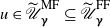

4.2.
$\widetilde{\mathscr{U\,}}^{\mathrm{MF}}_{\unicode{x1D6C4}}$
and the partial greediness

In this section we provide several tools based on the partial greediness
 $G_{\mathrm{par}}(u;\cdot)$
to verify whether a given function
 $u \in \widetilde{\mathscr{U\,}}^{\mathrm{FF}}_{\unicode{x1D6C4}}$
belongs to the multi-fractional utility space
 $\widetilde{\mathscr{U\,}}^{\mathrm{MF}}_{\unicode{x1D6C4}}$
. The underlying principle relies on the observation in Remark 7: for a function
 $\unicode{x1D6C4}$
, the space
 $\widetilde{\mathscr{U\,}}^{\mathrm{FF}}_{\unicode{x1D6C4}}$
contains more non-concave functions than
 $\mathscr{U\,}^{\mathrm{MF}}_{\unicode{x1D6C4}}$
. Therefore, given a function u, we use partial greediness to assess its degree of non-concavity and, in turn, determine whether it belongs to
 $\widetilde{\mathscr{U\,}}^{\mathrm{MF}}_{\unicode{x1D6C4}}$
. First, we start with the following lemma.
Lemma 3. Let
 $\unicode{x1D6C4}\colon \mathbb{R} \to [0, 1]$
be an arbitrary non-decreasing function. Let
 $u=\sum_{k=1}^{n} \lambda_k u_k \in \widetilde{\mathscr{U\,}}^{\mathrm{MF}}_{\unicode{x1D6C4}}$
,
 $n\in \mathbb{N}$
,
 $\lambda_k \ge 0$
, and
 $u_k \in \widetilde{\mathscr{U\,}}^{\mathrm{Union}}_{\unicode{x1D6C4}}$
,
 $k=1,\dots,n$
. Assume that there exists
 $x_0 \in \mathbb{R}$
such that
 $\unicode{x1D6C4}(x_0) \neq 0$
and, moreover,
 \begin{equation*} G_{\mathrm{par}}(u;\,x_0) = \dfrac{1}{\unicode{x1D6C4}(x_0)}.\end{equation*}
Then there exists an index
 $1 \le j \le n$
so that
 \begin{equation*}G_{\mathrm{par}}(u;\,x_0) = G_{\mathrm{par}}(u_j;\,x_0) =\max_{1 \le k\le n} G_{\mathrm{par}}(u_k;\,x_0) =\dfrac{1}{\unicode{x1D6C4}(x_0)}.\end{equation*}
The main message of Lemma 3 is that for
 $u \in \widetilde{\mathscr{U\,}}^{\mathrm{MF}}_{\unicode{x1D6C4}}$
,
 $G_{\mathrm{par}}(u;\,x)$
touches the upper bound given in (13) at
 $x_0$
if and only if u has an extreme component belonging to
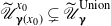 $\widetilde{\mathscr{U\,}}^{x_0}_{\unicode{x1D6C4}(x_0)} \subsetneq \widetilde{\mathscr{U\,}}^{\mathrm{Union}}_{\unicode{x1D6C4}}$
. We proceed with the following proposition, which asserts that for any
 $u \in \widetilde{\mathscr{U\,}}^{\mathrm{MF}}_{\unicode{x1D6C4}}$
, the upper bound for greediness (non-concavity) is reached only when
 $\boldsymbol{ \gamma}$
is constant in a neighbourhood of that point. The usefulness of this proposition becomes evident in the subsequent corollary, which states that if
 $G_{\mathrm{par}}(u;\,x)$
reaches the upper bound at some point and
 $\boldsymbol{ \gamma}$
is not constant around that point, then u cannot belong to
 $\widetilde{\mathscr{U\,}}^{\mathrm{MF}}_{\unicode{x1D6C4}}$
. It is important to note that such conditions are not required for functions in
 $\widetilde{\mathscr{U\,}}^{\mathrm{FF}}_{\unicode{x1D6C4}}$
.
Proposition 17. Let
 $\unicode{x1D6C4}\colon \mathbb{R} \to [0, 1]$
be an arbitrary non-decreasing function. Assume that
 $u \in \widetilde{\mathscr{U\,}}^{\mathrm{MF}}_{\unicode{x1D6C4}}$
and there exists
 $x_0 \in \mathbb{R}$
such that
 $\unicode{x1D6C4}(x_0) \neq 0$
and, moreover,
 \begin{equation*} G_{\mathrm{par}}(u;\,x_0) = \dfrac{1}{\unicode{x1D6C4}(x_0)}.\end{equation*}
Then there exists an open interval
 $I=I_{x_0} = (x_0,x_0+\delta)$
for some
 $\delta >0$
such that
 $\unicode{x1D6C4}$
is a constant function on I.
Corollary 2. Let
 $\unicode{x1D6C4}\colon \mathbb{R} \rightarrow [0, 1]$
be an arbitrary non-decreasing function such that there exists an open subset
 $U \subseteq \mathbb{R}$
where
 $\unicode{x1D6C4}$
is strictly increasing on U. Assume that
 $u \in \widetilde{\mathscr{U\,}}^{\mathrm{FF}}_{\unicode{x1D6C4}}$
and there exists
 $x_0 \in U$
such that
 \begin{equation*} G_{\mathrm{par}}(u;\, x_0)=\dfrac{1}{\boldsymbol{ \gamma}(x_0)}.\end{equation*}
Then
 $u \notin\widetilde{\mathscr{U\,}}^{\mathrm{MF}}_{\unicode{x1D6C4}}$
.
Next we present the main result of this section, which states that if, for a given
 $u \in \widetilde{\mathscr{U\,}}^{\mathrm{FF}}_{\unicode{x1D6C4}}$
, the partial greediness
 $G_{\mathrm{par}}(u;\, x)$
touches the upper bound for at least two distinct values of the function
 $\boldsymbol{ \gamma}$
, then
 $u \not\in \widetilde{\mathscr{U\,}}^{\mathrm{MF}}_{\unicode{x1D6C4}}$
. This follows because, for
 $u \in \widetilde{\mathscr{U\,}}^{\mathrm{MF}}_{\unicode{x1D6C4}}$
, once
 $G_{\mathrm{par}}(u;\, x)$
reaches its upper bound at a certain point x due to the extreme component (as per Lemma 3), u must remain constant thereafter. If not, the linear structure of
 $\widetilde{\mathscr{U\,}}^{\mathrm{MF}}_{\unicode{x1D6C4}}$
implies that combining this extreme component with other functions that are not constant after x – i.e. those unable to exhibit as steep non-concave segments – would detract the degree of non-concavity of u at x. Conversely, by the definition of the
 ${\boldsymbol{{D}}}_{\pm}(\unicode{x1D6C4})$
property, this does not apply to the functions within
 $\widetilde{\mathscr{U\,}}^{\mathrm{FF}}_{\unicode{x1D6C4}}$
.
Theorem 4. Let
 $\unicode{x1D6C4}\colon \mathbb{R} \to [0, 1]$
be an arbitrary non-decreasing function. Assume that
 $u \in \widetilde{\mathscr{U\,}}^{\mathrm{FF}}_{\unicode{x1D6C4}}$
and that there exist
 $x_0, x_1 \in \mathbb{R}$
such that
 $0 < \unicode{x1D6C4}(x_0) \neq \unicode{x1D6C4}(x_1)<1$
and
 \begin{equation*} G_{\mathrm{par}}(u;\,x_k) = \dfrac{1}{\unicode{x1D6C4}(x_k)}, \quad k=0,1.\end{equation*}
Then
 $u \notin \widetilde{\mathscr{U\,}}^{\mathrm{MF}}_{\unicode{x1D6C4}}$
.
We conclude this section with the following corollary, which provides the last piece of the overall framework. From Proposition 17 we already know that for a given u, if
 $G_{\mathrm{par}}(u;\,x_0)$
reaches the upper bound around a point where
 $\boldsymbol{ \gamma}$
is strictly increasing, then u cannot belong to
 $\widetilde{\mathscr{U\,}}^{\mathrm{MF}}_{\unicode{x1D6C4}}$
. Furthermore, this corollary establishes that when
 $\boldsymbol{ \gamma}$
is a piecewise constant function, and
 $G_{\mathrm{par}}(u;\,x)$
attains the upper bound for more than one value of
 $\boldsymbol{ \gamma}$
, then u does not lie in
 $\widetilde{\mathscr{U\,}}^{\mathrm{MF}}_{\unicode{x1D6C4}}$
.
Corollary 3. Let
 $\unicode{x1D6C4}\colon \mathbb{R} \to [0, 1]$
be a piecewise step function of the form given in (6). Assume that
 $u \in \widetilde{\mathscr{U\,}}^{\mathrm{FF}}_{\unicode{x1D6C4}}$
and that there exist
 $x_i \in (t_{i-1},t_i)$
and
 $x_j \in (t_{j-1},t_j)$
, where
 $1 \le i \neq j \le n$
such that
 \begin{equation*}G_{\mathrm{par}} (u;\,x_k) = \dfrac{1}{\unicode{x1D6C4}(x_k)}, \quad k=i,j.\end{equation*}
Then
 $u\notin \widetilde{\mathscr{U\,}}^{\mathrm{MF}}_{\unicode{x1D6C4}}$
.
4.3. Average risk aversion
In the preceding sections we explored the implications of the function
 $\boldsymbol{ \gamma}$
from an economics perspective, emphasizing non-differentiable utility functions. Now our focus shifts to differentiable utility functions, specifically strictly increasing twice-differentiable utility functions within
 $\widetilde{\mathscr{U\,}}^{\mathrm{FF}}_{\unicode{x1D6C4}}$
. In this context, the function
 $\boldsymbol{ \gamma}$
can be interpreted as a somewhat local lower bound on the average risk aversion (or an upper bound on risk loving behaviour) of a decision maker. Recall the well known Arrow–Pratt measure of absolute risk aversion (ARA) coefficient [Reference Arrow1, Reference Pratt26]:
 \begin{equation*}r_u(x) = r(x)\,:\!=\, -\dfrac{u^{\prime\prime}(x)}{u^{\prime}(x)}, \quad x\in \mathbb{R}.\end{equation*}
Then, invoking the classical Arrow–Pratt log–marginal–utility identity, one obtains a local (interval–average) lower bound on the average absolute risk aversion coefficient:
 \begin{equation}\int_x^y -\dfrac{u^{\prime\prime}(z)}{u^{\prime}(z)}{\mathrm{d}} z= [\!-{\ln}(u^{\prime}(y))+\ln(u^{\prime}(x))]={\ln}\biggl(\dfrac{u^{\prime}(x)}{u^{\prime}(y)}\biggr) \geq \ln\!(\unicode{x1D6C4}(y)) \quad \text{for all $x\le y$.}\end{equation}
Meyer [Reference Meyer21] generalizes SSD by restricting attention to decision makers whose Arrow–Pratt absolute risk aversion lies between prescribed lower and upper (wealth-dependent) bounds for all x. In the same vein, fractional degree SD [Reference Huang, Tzeng and Zhao10] provides a continuum between FSD and SSD via a global, constant bound on risk aversion/loving. However, (14) shows that the function
 $\unicode{x1D6C4}$
imposes an interval-average lower bound on absolute risk aversion on the entire interval [x, y] rather than pointwise.
When
 $\unicode{x1D6C4}(y)=0$
, the estimate becomes obvious since
 $\ln\!(\unicode{x1D6C4}(y))=-\infty$
. If u is fully concave then
 $r_u(x)\ge 0$
and the left-hand side is non-negative, so the inequality is immediate whenever
 $\unicode{x1D6C4}(y)\in(0,1]$
. In the more interesting case where u allows local non-concavity, the bound (14) quantifies risk attitudes on an average basis over [x, y]. Because
 $\unicode{x1D6C4}$
is non-decreasing, lower wealth levels permit (on average) more risk loving behaviour in the admissible classes
 $\widetilde{\mathscr{U\,}}^{\mathrm{FF}}_{\unicode{x1D6C4}}$
and
 $\widetilde{\mathscr{U\,}}^{\mathrm{MF}}_{\unicode{x1D6C4}}$
. This is consistent with the non-monotone curvature patterns proposed by [Reference Friedman and Savage9] and [Reference Markowitz20], which explain the coexistence of gambling and insurance and a wealth-dependent willingness to bear risk.
Another interesting observation is that when the function
 $\unicode{x1D6C4}$
is continuous, and by a direct application of the mean value theorem, in addition, we can observe that, for every x and every y in a tiny neighbourhood of x,
 \begin{equation*}\dfrac{\log \!( \unicode{x1D6C4} (x) ) }{y-x}\lessapprox r_u(x), \quad x \neq y.\end{equation*}
The latter heuristic observation interprets that the function
 $\unicode{x1D6C4}$
at each instance controls the non-concavity of the utility function u through the ARA coefficient. Similarly, one can discuss the relative absolute risk aversion coefficient
 $R_{u}(x)=-x({{u^{\prime\prime}(x)}/{u^{\prime}(x)}})$
as well.
In conclusion, it is evident that both the MFSD and FFSD methods utilize extra information regarding the position (wealth) of non-concave segments in the utility function u. Consequently, this approach enables a more comprehensive and realistic representation of decision makers’ behaviour, aligning with the expected utility theory.
5. Functional almost stochastic dominance
In this section we extend the concept of almost stochastic dominance (ASD), introduced in [Reference Leshno and Levy15]. This extension employs a combined concave/convex approach, parallelling the methodologies discussed in [Reference Müller, Scarsini, Tsetlin and Winkler23] within the framework of FFSD. Before proceeding, let us first recall the definition of the
 $\varepsilon$
-ASD utility space consisting of smooth functions,
 \begin{equation*}\mathscr{U\,}_{\varepsilon\textrm{-ASD}} = \biggl\{ u \colon \mathbb{R} \to \mathbb{R} \in C^{1}(\mathbb{R}) \colon 0 \le u^{\prime}(x) \le \inf_{x\in \mathbb{R}}u^{\prime(x)} \biggl[\dfrac{1-\varepsilon}{\varepsilon}\biggr]\ \text{for all } \textit{x} \biggr\},\end{equation*}
where
 $\varepsilon\in (0,1/2)$
. Inspired by the derivative-relation conditions given in (7), we obtain the following natural functional extension of the utility set
 $\mathscr{U\,}_{\varepsilon\textrm{-ASD}}$
through
 \begin{align}&{\rm (i)} \quad 0 \leq u'_-(x) \leq \inf_{x \in \mathbb{R}} u'_-(x) \biggl[\dfrac{1 - \unicode{x1D6DC}(x)}{\unicode{x1D6DC}(x)}\biggr] \quad \text{for all }\textit{x}, \end{align}
 \begin{align}&{\rm (ii)} \quad 0 \leq u'_+(x) \leq \inf_{x \in \mathbb{R}} u'_+(x) \biggl[\dfrac{1 - \unicode{x1D6DC}(x)}{\unicode{x1D6DC}(x)}\biggr] \quad \text{for all } \textit{x}, \end{align}
where
 $\unicode{x1D6DC}\colon \mathbb{R} \to (0,1/2)$
. Accordingly, we define the following property.
Definition 10. (
 ${\boldsymbol{{D}}}^{\mathrm{ASD}}_{\pm}(\unicode{x1D6DC})$
-property.) Let
 $\unicode{x1D6DC}\colon \mathbb{R} \to (0,1/2)$
be an arbitrary function. We say that a function
 $u\colon \mathbb{R} \to \mathbb{R}$
satisfies in
 ${\boldsymbol{{D}}}^{\mathrm{ASD}}_{\pm}(\unicode{x1D6DC})$
if it is two-sided differentiable and at least one of the conditions given in (15) and (16) holds.
Now we are ready for the formal definition.
Definition 11. (Functional
 $\unicode{x1D6DC}$
-ASD.) Let
 $\unicode{x1D6DC}\colon \mathbb{R} \to (0,1/2)$
be an arbitrary function. Let F and G be two distribution functions. We say that G dominates F in the sense of the functional
 $\unicode{x1D6DC}$
-ASD, denoted by
 $F \preceq_{\unicode{x1D6DC}\textrm{-ASD}} G$
, if
 \begin{equation*} \mathbb{E}_F [u] \le \mathbb{E}_G [u] \quad \text{for all $ u \in \widetilde{\mathscr{U\,}}^{\mathrm{ASD}}_{\unicode{x1D6DC}}$,}\end{equation*}
where
 \begin{equation*} \widetilde{\mathscr{U\,}}^{\mathrm{ASD}}_{\unicode{x1D6DC}} \,:\!=\, \bigl\{ u\colon \mathbb{R} \to \mathbb{R} \colon \textit{u}\text{ satisfies}\ {\boldsymbol{{D}}}^{\mathrm{ASD}}_{\pm}(\unicode{x1D6DC}) \bigr\},\end{equation*}
whenever the expectations exist.
Following the approach used in the proof of Proposition 11, we can demonstrate that setting
 $\unicode{x1D6DC}\equiv \varepsilon \in (0,1/2)$
results in the equality
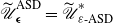 $\widetilde{\mathscr{U\,}}^{\mathrm{ASD}}_{\unicode{x1D6DC}} = \widetilde{\mathscr{U\,}}^*_{\varepsilon\textrm{-ASD}}$
. Here
 $\mathscr{U\,}^*_{\varepsilon\textrm{-ASD}}$
represents the set of non-differentiable utility functions associated with
 $\varepsilon$
-ASD. Furthermore, a close examination of conditions (15) and (16) shows that the function
 $\unicode{x1D6DC}$
controls the maximal possible jump in the one-sided derivatives at a given location x. This control is highly localized, meaning its impact does not extend to values other than x, unlike other orders introduced so far. For instance, at those points where
 $\unicode{x1D6DC}(x)\approx 0$
, utility functions in
 $\widetilde{\mathscr{U\,}}^{\mathrm{ASD}}_{\unicode{x1D6DC}}$
may exhibit greater jumps in their one-sided derivatives compared to points where
 $\unicode{x1D6DC}(x)\approx \frac{1}{2}$
, at which the one-sided derivatives are constrained to be closer to their infimum. Also, note that any
 $u \in \widetilde{\mathscr{U\,}}^{\mathrm{ASD}}_{\unicode{x1D6DC}}$
is either a constant function or strictly increasing. It is evident that, for any chosen function
 $\unicode{x1D6DC}\colon \mathbb{R} \to (0,1/2)$
, the set
 $\widetilde{\mathscr{U\,}}^{\mathrm{ASD}}_{\unicode{x1D6DC}}$
is non-empty, and it is easy to verify whether a given utility function belongs to it. Moreover, it is always possible to choose an appropriate
 $\unicode{x1D6DC}$
for specific purposes, without restricting the selection to solely monotone functions. Next, we present the ‘if and only if’ theorem along with the corresponding integral condition for a given
 $\unicode{x1D6DC}\colon \mathbb{R} \to (0,1/2)$
, as follows:
 \begin{equation}\int_{-\infty}^\infty \dfrac{1}{\unicode{x1D6DC}(x)} (F(x)-G(x))_-{\mathrm{d}} x \le \int_{-\infty}^\infty |(F(x)-G(x))|{\mathrm{d}} x.\end{equation}
Before proceeding, we give the following remark, which highlights a few important points.
Remark 16.
-
(i) We give the proof without assuming monotonicity on
$\unicode{x1D6DC}$
and avoid arguments relying on the first crossing point of given distribution functions. To ensure the integral condition is meaningful and avoid potential technical difficulties, we consider a restricted subset of pairs of distribution functions. For a given
$\unicode{x1D6DC}\colon \mathbb{R} \to (0,1/2)$
, we define
\begin{equation*}\operatorname{L}^1(\unicode{x1D6DC})\,:\!=\, \biggl\{F,G\in \unicode{x1D4D3}\,(\mathbb{R})\colon \int_{-\infty}^{\infty}\biggl|\dfrac{1}{\unicode{x1D6DC}(x)} (F(x)-G(x))_-\biggr|\,{\mathrm{d}} x<\infty\biggr\}.\end{equation*}
-
(ii) The integral condition (17) can be equivalently represented as
\begin{equation*} \int_{-\infty}^\infty \dfrac{1-\unicode{x1D6DC}(x)}{\unicode{x1D6DC}(x)} (F(x)-G(x))_-{\mathrm{d}} x \le \int_{-\infty}^\infty (F(x)-G(x))_+{\mathrm{d}} x.\end{equation*}
-
(iii) Building on the approach detailed in Remark 8(ii) for FFSD, we prove one direction of the theorem under the additional assumptions regarding both
$\boldsymbol{ \epsilon}$
and the crossing points of the given distribution functions. -
(iv) To focus on essential aspects of the proof and avoid unnecessary discussion, we assume
$\mathbb{E}_F[|u|],\mathbb{E}_G[|u|]<\infty$
for all
$u \in \widetilde{\mathscr{U\,}}^{\mathrm{ASD}}_{\unicode{x1D6DC}}$
.






Theorem 5. Let
 $\unicode{x1D6DC}\colon \mathbb{R} \to (0,1/2)$
be an arbitrary right-continuous function with finitely many jumps and one-sided limits at each point. Let F and G be distribution functions in
 $\operatorname{L}^1(\unicode{x1D6DC})$
that cross finitely many times. Then
 $F \preceq_{\unicode{x1D6DC}\textrm{{-ASD}}} G$
if and only if the integral condition (17) holds.
We conclude that the utility class
 $\widetilde{\mathscr{U\,}}^{\mathrm{ASD}}_{\unicode{x1D6DC}}$
admits an integral condition, leading to functional
 $\unicode{x1D6DC}$
-ASD as a meaningful ordering relation. This extension may be beneficial for broader applications and interpretations across various contexts, particularly in scenarios where the traditional
 $\varepsilon$
-ASD falls short.
6. Conclusion
In this paper we propose a twofold generalization of fractional stochastic dominance by replacing the fixed parameter
 $\gamma$
with a non-decreasing function
 $\unicode{x1D6C4}\colon \mathbb{R} \rightarrow [0, 1]$
. This leads to the introduction of two novel families, MFSD and FFSD. These generalizations effectively interpolate between FSD and SSD, thereby addressing their limitations. Unlike fractional SD, which provides only global interpolation, our approach enables more informative local interpolation. This distinction allows MFSD and FFSD to rank distributions that are otherwise indistinguishable under fractional SD. Moreover, the corresponding utility classes consist of functions with local non-concavities, where the steepness of the convexities is controlled by the function
 $\unicode{x1D6C4}$
.
Another contribution of our framework is the introduction of partial greediness, which captures the evolution of greediness behaviour with changes in wealth. As wealth increases, decision makers exhibit diminishing greediness, reflected in the non-increasing bounds defined by
 $\unicode{x1D6C4}$
. Partial greediness also serves as a practical criterion for identifying whether a utility function falls under MFSD or FFSD. Additionally, we extend the same analysis to risk-taking behaviour through the bounding relationship of average risk aversion, offering insights that fractional SD cannot provide due to its reliance on a fixed
 $\gamma$
. Lastly, we provide a generalized family of FASD that extends the results of ASD.
We have introduced a novel framework for understanding choice under uncertainty, providing a more comprehensive and flexible approach than traditional methods. Our extension offers a methodology that contributes to the literature and opens new avenues for research and practical applications across a range of fields. Future research could examine the use of these generalizations in specific economic models, such as portfolio optimization and behavioural economics, and explore their implications for decision-making under uncertainty. There is also substantial potential for applications in actuarial science, particularly in risk assessment, where the ability to compare risk distributions is critical.
Acknowledgement
The authors are grateful to the two anonymous reviewers for their constructive and insightful comments, which have helped to improve the manuscript.
Funding information
This work presents research originally included in Ozan Hür’s PhD thesis [Reference Hür11], completed at the University of Liverpool under the supervision of Ehsan Azmoodeh. We acknowledge the funding provided by the University of Liverpool during the doctoral research that made this work possible.
Competing interests
There were no competing interests to declare which arose during the preparation or publication process of this article.
Supplementary material
The supplementary material for this article can be found at https://doi.org/10.1017/jpr.2026.10111.

 F=N(0,1)
 G=N(μG,σG2)
 Δμ/Δσ
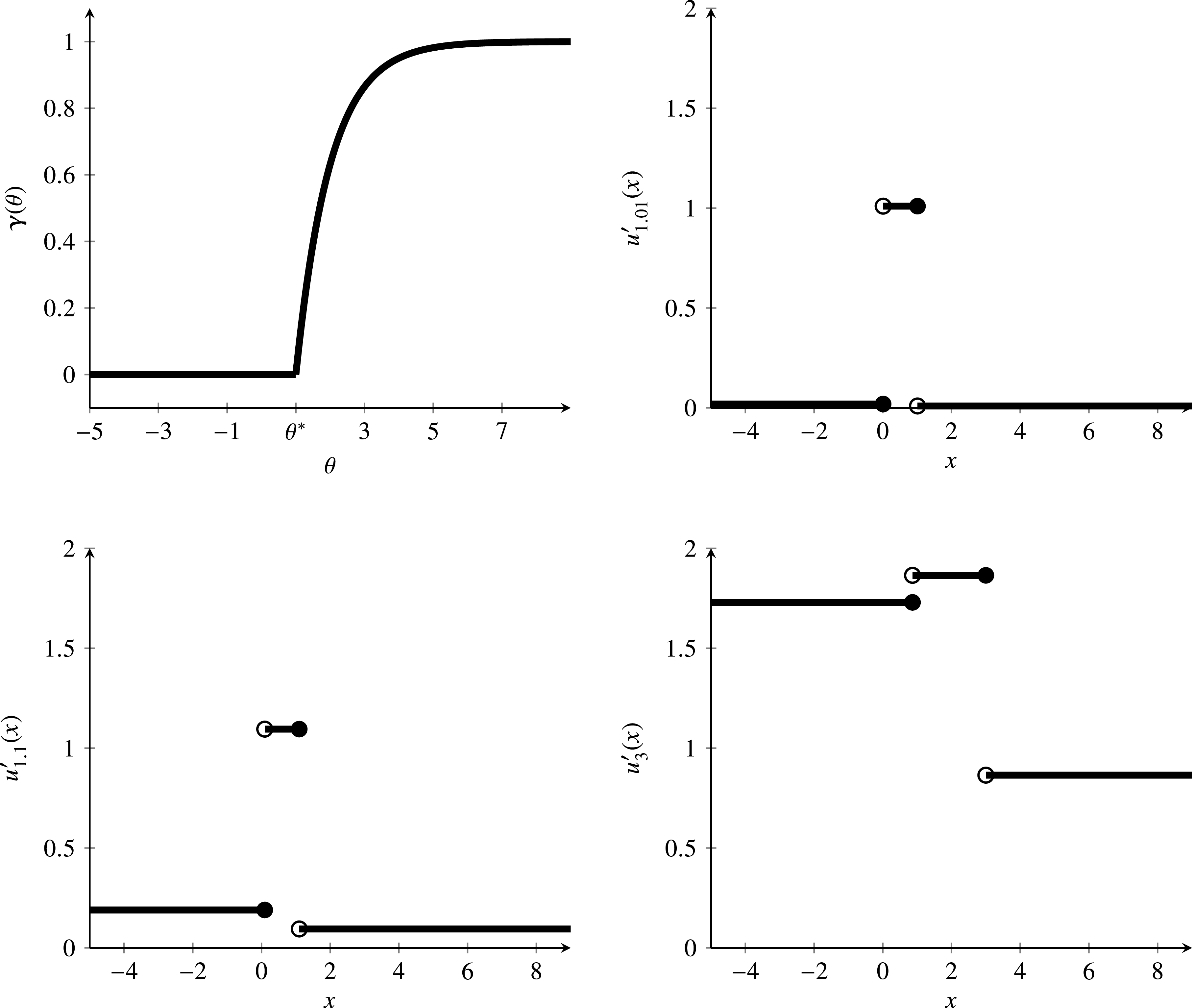
 uθ′
 θ=1.01
 θ=1.1
 θ=3
 𝛄
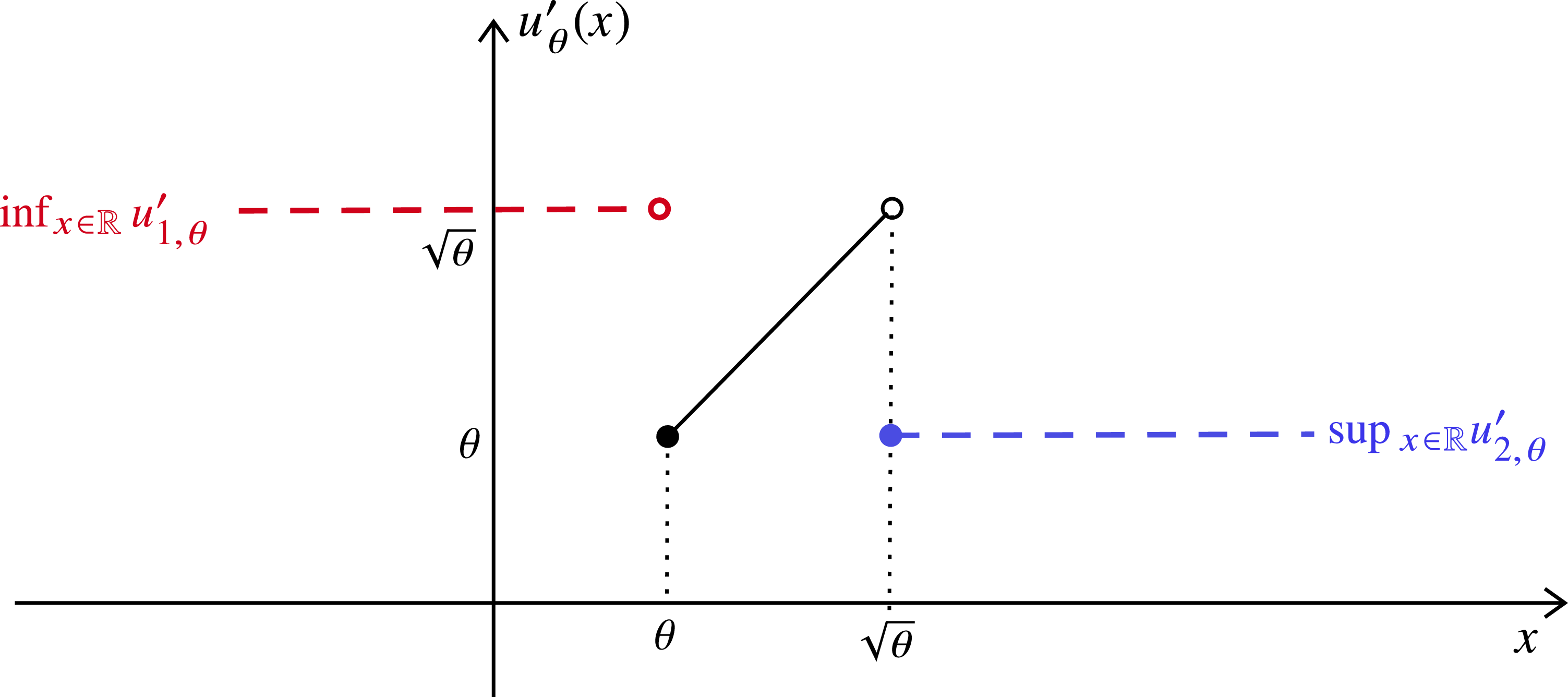
 uθ′


 Open access

