


1. Introduction
Series–parallel systems arise across critical infrastructures such as power networks, manufacturing lines, telecommunication architectures, and supply chains where components within the same subsystem often share environmental stressors that classical independent-failure models cannot represent. The Marshall–Olkin (MO) framework [Reference Marshall and Olkin15] provides a natural mechanism for such dependence: each component is exposed to a private shock source affecting only that component and to a common shock source shared by all components in the same block, so that failure occurs when either source accumulates sufficient damage. When shock damage is governed by a run mechanism requiring  $k$ consecutive critical shocks rather than a single harmful event [Reference Mallor and Omey14], the model captures the inherent resilience of engineered systems to isolated stressors while remaining analytically tractable through the theory of phase-type (PH) distributions [Reference Assaf and Levikson2, Reference He13, Reference Neuts18].
Run shock models have been developed in several directions, including discrete-time formulations [Reference Eryilmaz9], generalized  $\delta$-shock variants [Reference Eryilmaz8], and Polya process arrivals [Reference Eryilmaz10]. Closely related
 $\delta$-shock models include the system reliability analysis of Tuncel and Eryilmaz [Reference Tuncel and Eryilmaz28] and the mixed
 $\delta$-shock model with a change in shock distribution of Chadjiconstantinidis et al. [Reference Chadjiconstantinidis, Tuncel and Eryilmaz6]. Eryilmaz and Kan [Reference Eryilmaz and Kan11] extended the run shock concept by allowing the shock size distribution to change after the first shock exceeding a warning threshold, establishing that the resulting system lifetime has a matrix-exponential distribution when interarrival times follow an Erlang law. More recently, Ozkut et al. [Reference Ozkut, Kan and Franko23] developed a multi-state system model in which runs of shocks cause partial damage before complete system failure. Fan and Tang [Reference Fan and Tang12] studied a mixed run shock model that combines run shocks, extreme shocks, and degradation, and used phase-type distributions to evaluate the hard failure process. A recent review of MO shock models and their applications in reliability is given by Bayramoglu and Ozkut [Reference Bayramoglu and Ozkut5]. Bakry and Mokhlis [Reference Bakry and Mokhlis3] studied the reliability of a
 $k$-out-of-
 $n$:G system exposed to component-specific and common MO shocks, while also accounting for shock magnitudes. MO type shock models have also been studied by Ozkut and Bayramoglu [Reference Ozkut and Bayramoglu20], Bayramoglu and Ozkut [Reference Bayramoglu and Ozkut4], Rafiee et al. [Reference Rafiee, Feng and Coit24], and Durante et al. [Reference Durante, Girard and Mazo7]. Phase-type distributions, whose closure properties under minimum, maximum, and random summation have been applied to shock models by Montoro-Cazorla et al. [Reference Montoro-Cazorla, Pérez-Ocón and Segovia16, Reference Montoro-Cazorla, Pérez-Ocón and Segovia17] and Segovia and Labeau [Reference Segovia and Labeau25], and to two-component systems by Neuts and Meier [Reference Neuts and Meier19]. More recently, Wang et al. [Reference Wang, Zhao, Zhao, Chen and Ning30] used phase-type distributions to study a heterogeneous system exposed to several shock sources under a mixed shock model. Recent work by Torrado and Ozkut [Reference Torrado and Ozkut27] considers series–parallel systems with dependent components. Ozkut and Kan [Reference Ozkut and Kan22] later applied the MO run shock model to coherent systems with phase-type shock interarrival times. Most relevantly, Ozkut and Eryilmaz [Reference Ozkut and Eryilmaz21] introduced the MO run shock model for a two-component system with PH interarrival times, deriving the joint survival function and mean residual life in closed matrix-exponential form.
The aim of this paper is twofold. First, we extend the MO run shock model from the two-component system of [Reference Ozkut and Eryilmaz21] to a general  $m$-block series–parallel system with an arbitrary number of parallel components per block. Second, we derive its reliability measures in closed matrix-exponential form. This is not a routine application of known closure results. The parallel blocks create a dependence that blocks the standard phase-type maximum closure, and removing this obstacle requires the new decomposition lemma below. The paper also proves a new invariance property of the conditional mean residual life. We state both contributions precisely in what follows.
The present paper addresses the natural but technically non-trivial extension of [Reference Ozkut and Eryilmaz21] to  $m$-block series–parallel systems in which each block contains an arbitrary number
 $n_i \geq 1$ of parallel components. This extension introduces a fundamental obstacle absent from [Reference Ozkut and Eryilmaz21]. In [Reference Ozkut and Eryilmaz21], every block contains a single component, so all random variables involved are independent and only the PH minimum closure is needed. Once a block contains
 $n_i \geq 2$ parallel components that share a common run-shock time
 $T_{iC}(k)$, the component lifetimes within the block become dependent through this shared term. Direct application of the PH maximum closure, which requires independence of its arguments, is therefore blocked. Lemma 4.1 resolves this obstacle by establishing the representation
 \begin{equation*}
S_i \;=\; \min\!\Bigl\{T_{iC}(k),\;\max_{1 \leq j \leq n_i} T_{ij}(k)\Bigr\},
\end{equation*}
which expresses the block lifetime entirely in terms of mutually independent run-shock times, restoring full applicability of the PH closure machinery. This lemma is the structural hinge on which the entire hierarchical construction rests, and it has no counterpart in [Reference Ozkut and Eryilmaz21]. A second contribution, developed in Section 5, establishes that the conditional mean residual life of any component given the survival of all other components in its block depends on their observation times only through their maximum, a structural invariance property specific to the MO parallel-block architecture with no direct analog in independent-failure models.
The main contributions of this work are as follows.
(i) A structural decomposition that overcomes the dependence obstacle created by shared common shocks in parallel blocks. By reformulating each block lifetime in terms of independent run-shock times, the PH maximum closure, an operation not required in [Reference Ozkut and Eryilmaz21], becomes applicable, yielding exact phase-type representations for block lifetimes via nested Kronecker products.
(ii) Exact phase-type representations for component, block, and system lifetimes under the MO run shock mechanism, generalizing [Reference Ozkut and Eryilmaz21] from a single-block pair to an arbitrary series–parallel architecture with
 $n_i \geq 1$ parallel components per block.
(iii) Survival functions, mean time to failure, variance, hazard rate, and mean residual life are computable without Monte Carlo simulation (equations (17)–(19) and Theorem 4.5).
(iv) Explicit matrix-exponential formulas for the conditional MRL of any component given multi-component survival observations within the same block, together with the maximum-observation-time invariance property (Corollary 5.1).
(v) Closed-form expressions quantifying how state-space complexity scales with the number of blocks, components per block, phase dimensions, and the run-length threshold
$k$.


We close the introduction by stating how these contributions relate to the existing literature. The two-component model of [Reference Ozkut and Eryilmaz21] is the closest work. There, every block holds a single component, so the component lifetimes are independent and only the phase-type minimum closure is used. Our model allows any number of parallel components per block. This makes the within-block lifetimes dependent and forces the use of the maximum closure, and Lemma 4.1 is what makes this step possible. This lemma does not appear in [Reference Ozkut and Eryilmaz21]. The run shock model with a change in shock size distribution of Eryilmaz and Kan [Reference Eryilmaz and Kan11] treats a single component and a different mechanism, so the dependence studied here does not arise there. Phase-type methods have been used for shock and wear models by [Reference Montoro-Cazorla, Pérez-Ocón and Segovia16, Reference Montoro-Cazorla, Pérez-Ocón and Segovia17, Reference Segovia and Labeau25] and for two-component systems by Neuts and Meier [Reference Neuts and Meier19], but not for the MO run shock model on a general series–parallel architecture with block-common shocks. Recent studies have also used phase-type methods for mixed run shocks and multi-source shock environments [Reference Fan and Tang12, Reference Wang, Zhao, Zhao, Chen and Ning30]. However, their failure mechanisms and system structures differ from the block-common MO setting considered here. The maximum closure we use follows the generalized geometric results of Tank and Eryilmaz [Reference Tank and Eryilmaz26]. To our knowledge, the conditional MRL invariance in Corollary 5.1, which says that the companion observations enter only through their maximum, has not been reported before.
The paper is organized as follows. Section 2 collects the necessary PH distribution theory and Kronecker algebra. Section 3 defines the system model and shock structure. Section 4 derives the hierarchical reliability construction. Section 5 develops the conditional MRL results. Section 6 presents a numerical illustration. Section 7 concludes.
2. Mathematical preliminaries
Throughout,  $\mathbf{1}_n$ denotes the
 $n\times 1$ vector of ones,
 $I_n$ the
 $n\times n$ identity matrix, and
 $\otimes$ the Kronecker product.
2.1. Phase-type distributions
Definition 2.1. A non-negative continuous random variable  $X$ has a continuous phase-type distribution, written
 $X\sim\mathrm{PH}_c(\alpha,A)$, if it represents the time to absorption in a continuous-time Markov chain with
 $m$ transient states and one absorbing state. The subgenerator matrix
 $A\in\mathbb{R}^{m\times m}$ satisfies
 $a_{ii} \lt 0$,
 $a_{ij}\geq 0$ for
 $i\neq j$, and
 $A\mathbf{1}_m\leq\mathbf{0}_m$; the initial vector
 $\alpha\in\mathbb{R}^{1\times m}$ satisfies
 $\alpha\mathbf{1}_m\leq 1$. The survival function is
 \begin{equation}
\bar{F}_X(t)=P(X \gt t)=\alpha\exp(At)\mathbf{1}_m,\qquad t\geq 0.
\end{equation}
The integer  $m$ is called the order of the representation.
The class of continuous phase-type distributions includes exponential, Erlang, hypoexponential, and hyperexponential distributions as special cases and is dense in the set of all distributions on  $(0,\infty)$ [Reference Aalen1].
Proposition 2.1 ([Reference He13])
Let  $X\sim\mathrm{PH}_c(\alpha,A)$ with
 $\alpha\mathbf{1}_m=1$. Then
 \begin{equation*}
E[X^n]=(-1)^n\,n!\;\alpha A^{-n}\mathbf{1}_m, \qquad n\in\mathbb{N}.
\end{equation*}
In particular,  $E[X]=-\alpha A^{-1}\mathbf{1}_m$ and
 $\operatorname{Var}(X)=2\alpha A^{-2}\mathbf{1}_m-({\alpha A^{-1}\mathbf{1}_m})^2$.
Proposition 2.2 ([Reference He13])
Let  $X\sim\mathrm{PH}_c(\alpha,A)$. For
 $t \gt 0$, the conditional residual lifetime satisfies
 \begin{equation*}
(X-t\mid X \gt t)\sim\mathrm{PH}_c\!\left(
\frac{\alpha\exp(At)}{\alpha\exp(At)\mathbf{1}_m},\;A\right).
\end{equation*}
In particular, the mean residual life function is
 \begin{equation*}
E[X-t\mid X \gt t]
=\frac{-\alpha\exp(At)A^{-1}\mathbf{1}_m}{\alpha\exp(At)\mathbf{1}_m}.
\end{equation*}
Definition 2.2. Let  $A\in\mathbb{R}^{m\times m}$ and
 $B\in\mathbb{R}^{n\times n}$. The Kronecker product
 $A\otimes B\in\mathbb{R}^{mn\times mn}$ is the block matrix with
 $(i,j)$-block
 $a_{ij}B$. The Kronecker sum is
 \begin{equation*}
A\oplus B:=A\otimes I_n + I_m\otimes B\;\in\mathbb{R}^{mn\times mn}.
\end{equation*}
Lemma 2.1. For  $A\in\mathbb{R}^{m\times m}$ and
 $B\in\mathbb{R}^{n\times n}$,
 \begin{equation*}
\exp\ \bigl((A\oplus B)t\bigr)=\exp(At)\otimes\exp(Bt),\qquad t\geq 0.
\end{equation*}
Proof. The matrices  $A\otimes I_n$ and
 $I_m\otimes B$ commute, since by the mixed-product rule
 $(A\otimes I_n)(I_m\otimes B)=A\otimes B=(I_m\otimes B)(A\otimes I_n)$. For commuting matrices, the exponential of a sum factors as a product, so
 $\exp((A\oplus B)t)=\exp((A\otimes I_n)t)\,\exp((I_m\otimes B)t)$. Each factor is
 $\exp(At)\otimes I_n$ and
 $I_m\otimes\exp(Bt)$, and the mixed-product rule gives their product as
 $\exp(At)\otimes\exp(Bt)$. See [Reference He13] for details.
The following three propositions establish the closure results on which the entire hierarchical construction in Section 4 rests.
Proposition 2.3 ([Reference Assaf and Levikson2, Reference He13])
Let  $X\sim\mathrm{PH}_c(\alpha_X,A_X)$ and
 $Y\sim\mathrm{PH}_c(\alpha_Y,A_Y)$ be independent, with dimensions
 $r_X$ and
 $r_Y$. Then
 \begin{equation*}
\min(X,Y)\sim\mathrm{PH}_c(\alpha_X\otimes\alpha_Y,\;A_X\oplus A_Y),
\end{equation*}
with dimension  $r_X r_Y$.
Proposition 2.4 ([Reference He13, Reference Tank and Eryilmaz26])
Under the same conditions as Proposition 2.3, define  $t_0=-A_X\mathbf{1}_{r_X}$ and
 $s_0=-A_Y\mathbf{1}_{r_Y}$. Then
 \begin{equation*}
\max(X,Y)\sim\mathrm{PH}_c(\gamma,L),
\end{equation*}
where
 \begin{equation*}
\gamma=\bigl(\alpha_X\otimes\alpha_Y,\;
\alpha_X(1-\alpha_Y\mathbf{1}_{r_Y}),\;
(1-\alpha_X\mathbf{1}_{r_X})\alpha_Y\bigr)
\in\mathbb{R}^{1\times(r_Xr_Y+r_X+r_Y)},
\end{equation*}
 \begin{equation*}
L=\begin{pmatrix}
A_X\oplus A_Y & I_{r_X}\otimes s_0 & t_0\otimes I_{r_Y}\\
0 & A_X & 0 \\
0 & 0 & A_Y
\end{pmatrix}
\in\mathbb{R}^{(r_Xr_Y+r_X+r_Y)\times(r_Xr_Y+r_X+r_Y)}.
\end{equation*}
The dimension of  $\max(X,Y)$ is
 $(r_X+1)(r_Y+1)-1$.
Remark 2.1. The minimum closure gives dimension  $r_Xr_Y$ (multiplicative), while the maximum closure gives
 $(r_X+1)(r_Y+1)-1$ (strictly larger). For systems with substantial parallel redundancy, state-space growth is dominated by iterated maximum operations.
Proposition 2.5 ([Reference He13])
Let  $\{X_i\}_{i\geq 1}$ be i.i.d. with
 $X_i\sim\mathrm{PH}_c(\alpha,A)$ of dimension
 $d$ and
 $\alpha\mathbf{1}_d=1$, and let
 $N$ be an independent counting random variable having a discrete phase-type distribution
 $N\sim\mathrm{PH}_d(a,Q)$ of dimension
 $k$ with
 $a\mathbf{1}_k=1$ (i.e.,
 $N$ is the absorption time in a discrete-time Markov chain with substochastic transition matrix
 $Q$). Then
 \begin{equation*}
T=\sum_{i=1}^{N}X_i
\sim\mathrm{PH}_c\!\bigl(\alpha\otimes a,\;
A\otimes I_k+(a_0\alpha)\otimes Q\bigr),
\end{equation*}
where  $a_0=-A\mathbf{1}_d$, with dimension
 $dk$.
2.2. Geometric distribution of order
$k$

The run shock mechanism requires counting the number of Bernoulli trials until  $k$ consecutive successes first occur; this counting variable follows the geometric distribution of order
 $k$ [Reference He13].
Proposition 2.6 ([Reference He13])
Let  $\{Y_i\}_{i\geq 1}$ be i.i.d. Bernoulli with success probability
 $p\in(0,1)$, and let
 $N$ be the total number of trials until
 $k$ consecutive successes occur. Then
 $N\sim\mathrm{PH}_d(a,Q)$ with
 $a=(1,0,\ldots,0)\in\mathbb{R}^{1\times k}$ and
 \begin{equation*}
Q=\begin{pmatrix}
1-p & p & 0 & \cdots & 0 & 0\\
1-p & 0 & p & \cdots & 0 & 0\\
1-p & 0 & 0 & \ddots & & 0\\
\vdots & & & \ddots & \ddots & \vdots\\
1-p & 0 & 0 & \cdots & 0 & p\\
1-p & 0 & 0 & \cdots & 0 & 0
\end{pmatrix}\in\mathbb{R}^{k\times k},
\end{equation*}
where state  $j\in\{1,\ldots,k\}$ represents a current run of
 $j-1$ consecutive successes, and absorption corresponds to reaching run length
 $k$.
3. System model
3.1. Series–parallel architecture
We consider a system of  $m$ blocks connected in series, where block
 $i$ contains
 $n_i \geq 1$ components connected in parallel (
 $i = 1, \ldots, m$;
 $j = 1, \ldots, n_i$). Let
 $S_{ij}$,
 $S_i$, and
 $T$ denote the lifetimes of component
 $(i,j)$, block
 $i$, and the system, respectively. The structural equations are
 \begin{equation}
S_i = \max_{1 \leq j \leq n_i} S_{ij}, \qquad
T = \min_{1 \leq i \leq m} S_i
= \min_{1 \leq i \leq m}\Bigl(\max_{1 \leq j \leq n_i} S_{ij}\Bigr).
\end{equation}
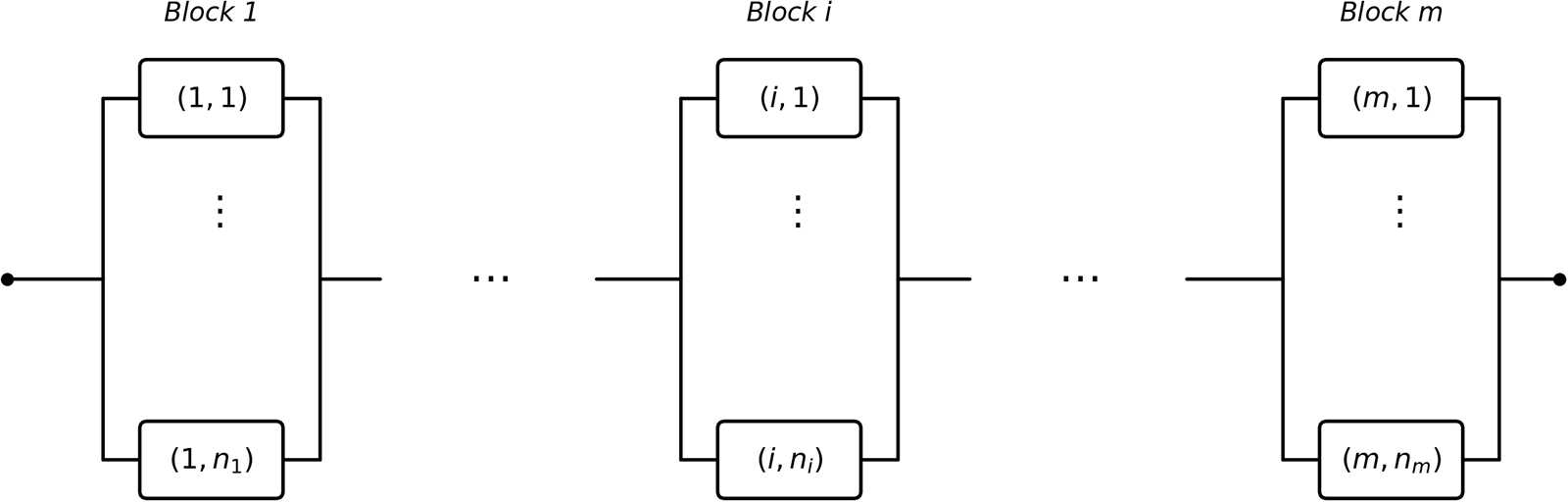
The block-size vector  $\boldsymbol{n}=(n_1,\ldots,n_m)$ fully characterizes the architecture; Figure 1 illustrates the general case.
Series–parallel system with  $m$ blocks in series, block
 $i$ containing
 $n_i$ parallel components.

3.2. Marshall–Olkin run shock mechanism
Definition 3.1 (Marshall–Olkin run shock model)
Each component  $(i,j)$ is subject to shocks from two mutually independent sources:
(a) Private source
$(i,j)$: affects only component
$(i,j)$, with i.i.d. interarrival times
$X_{ij,n} \sim \mathrm{PH}_c(\alpha_{ij},A_{ij})$ of phase dimension
$d_{ij}$, and critical shock probability
$p_{ij}\in(0,1)$.(b) Block-common source
$(i,C)$: shared by all
$n_i$ components in block
$i$, with i.i.d. interarrival times
$X_{iC,n} \sim \mathrm{PH}_c(\alpha_{iC},A_{iC})$ of phase dimension
$d_{iC}$, and critical shock probability
$p_{iC}\in(0,1)$.


Each shock from source  $r$ is independently classified as critical (with probability
 $p_r$) or non-critical (with probability
 $1-p_r$). A non-critical shock resets the consecutive-critical-shock counter to zero. Component
 $(i,j)$ fails when either source
 $(i,j)$ or source
 $(i,C)$ first accumulates
 $k \geq 1$ consecutive critical shocks. All shock processes across different sources are mutually independent.
The block-common source  $(i,C)$ induces positive dependence among the lifetimes of components within block
 $i$: any two components
 $(i,j)$ and
 $(i,j')$ with
 $j \neq j'$ share
 $T_{iC}(k)$, so their lifetimes are positively correlated. Components in different blocks share no common source and are therefore independent.
3.3. Run-shock time distributions
For source  $r$ with critical probability
 $p_r$, let
 $N_r(k)$ be the total number of shocks until
 $k$ consecutive critical shocks occur. By Proposition 2.6,
 $N_r(k) \sim \mathrm{PH}_d(\boldsymbol{a}, Q_r)$ with
 $\boldsymbol{a} = (1,0,\ldots,0) \in \mathbb{R}^{1 \times k}$ and
 \begin{equation}
Q_r = \begin{pmatrix}
1-p_r & p_r & 0 & \cdots & 0 \\
1-p_r & 0 & p_r & \cdots & 0 \\
\vdots & & \ddots & \ddots & \vdots \\
1-p_r & 0 & 0 & \cdots & p_r \\
1-p_r & 0 & 0 & \cdots & 0
\end{pmatrix} \in \mathbb{R}^{k \times k}.
\end{equation}
The run-shock time  $T_r(k) = \sum_{n=1}^{N_r(k)} X_{r,n}$ is the time until source
 $r$ first produces
 $k$ consecutive critical shocks. By Proposition 2.5,
 $T_r(k)$ has a phase-type distribution with explicit parameters:
Proposition 3.1. The run-shock time  $T_r(k)$ satisfies
 $T_r(k) \sim \mathrm{PH}_c(\boldsymbol{v}_r, Z_r)$, where
 \begin{equation}
\boldsymbol{v}_r = \alpha_r \otimes \boldsymbol{a},
\qquad
Z_r = A_r \otimes I_k + (\boldsymbol{a}_{0,r}\,\alpha_r) \otimes Q_r,
\end{equation}
with  $\boldsymbol{a}_{0,r} = -A_r \mathbf{1}_{d_r}$, and
 $\bar{d}_r := \dim(Z_r) = d_r \cdot k$.
Proof. We obtain the expression from the random-sum closure of Proposition 2.5. The run-shock time is the random sum  $T_r(k)=\sum_{n=1}^{N_r(k)}X_{r,n}$, where the interarrival times
 $X_{r,n}\sim\mathrm{PH}_c(\alpha_r,A_r)$ are i.i.d. of order
 $d_r$, and the shock count
 $N_r(k)$ is independent of the interarrival times. By Proposition 2.6,
 $N_r(k)$ has the discrete phase-type representation
 $\mathrm{PH}_d(\boldsymbol{a},Q_r)$ of order
 $k$, with
 $\boldsymbol{a}=(1,0,\ldots,0)$ and
 $Q_r$ given by (3). We now apply Proposition 2.5 with
 $\alpha=\alpha_r$,
 $A=A_r$,
 $\boldsymbol{a}=(1,0,\ldots,0)$, and
 $Q=Q_r$. With
 $\boldsymbol{a}_{0,r}=-A_r\mathbf{1}_{d_r}$, this gives the initial vector
 $\boldsymbol{v}_r=\alpha_r\otimes\boldsymbol{a}$ and the subgenerator
 $Z_r=A_r\otimes I_k+(\boldsymbol{a}_{0,r}\alpha_r)\otimes Q_r$ of order
 $\bar{d}_r=d_r k$, which is (4).
Applying Proposition 3.1 to every shock source gives
 \begin{equation}
T_{ij}(k) \sim \mathrm{PH}_c(\boldsymbol{v}_{ij}, Z_{ij}),
\quad \bar{d}_{ij} = d_{ij} k,
\qquad
T_{iC}(k) \sim \mathrm{PH}_c(\boldsymbol{v}_{iC}, Z_{iC}),
\quad \bar{d}_{iC} = d_{iC} k,
\end{equation}
for  $i = 1,\ldots,m$ and
 $j = 1,\ldots,n_i$. Under Definition 3.1, the lifetime of component
 $(i,j)$ is
 \begin{equation}
S_{ij} = \min\bigl\{T_{ij}(k),\; T_{iC}(k)\bigr\},
\qquad i = 1,\ldots,m;\; j = 1,\ldots,n_i.
\end{equation}
Equation (6) reflects the competing-risks structure: the component fails due to whichever source first accumulates  $k$ consecutive critical shocks. Phase-type representations for
 $S_{ij}$,
 $S_i$, and
 $T$ are derived in Section 4.
Example 3.1 (Explicit Erlang-2 building blocks)
We make the construction explicit for the Erlang $(2,\lambda)$ interarrival times and
 $k=2$ used in Section 6. Here
 $\alpha_r=(0,1)$,
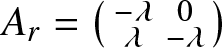 $A_r=\left(\begin{smallmatrix}-\lambda&0\\\lambda&-\lambda\end{smallmatrix}\right)$, so
 $\boldsymbol{a}_{0,r}=-A_r\mathbf{1}_2=(\lambda,0)^{\top}$, and the run matrix is
 $Q_r=\left(\begin{smallmatrix}1-p&p\\1-p&0\end{smallmatrix}\right)$. By (4), the run-shock time
 $T_r(2)$ has order
 $\bar{d}_r=4$ with
 \begin{equation}
\boldsymbol{v}_r=(0,0,1,0),
\qquad
Z_r=\begin{pmatrix}
-\lambda & 0 & \lambda(1-p) & \lambda p\\
0 & -\lambda & \lambda(1-p) & 0\\
\lambda & 0 & -\lambda & 0\\
0 & \lambda & 0 & -\lambda
\end{pmatrix}.
\end{equation}
The exit vector is  $-Z_r\mathbf{1}_4=(0,\lambda p,0,0)^{\top}$, so absorption occurs at rate
 $\lambda p$ from the single state in which one critical shock has already occurred, and the next interarrival is in its last phase. The component lifetime
 $S_{ij}=\min(T_{ij}(2),T_{iC}(2))$ then has the explicit order-
 $16$ representation (Theorem 4.1)
 $\alpha^{(S)}_{ij}=\boldsymbol{v}_{ij}\otimes\boldsymbol{v}_{iC}$ and
 $A^{(S)}_{ij}=Z_{ij}\oplus Z_{iC}$, where each factor has the form (7) with its own rate and probability. The block and system generators of Theorems 4.2 and 4.3, and the conditional MRL formulas (28)–(29) of Section 5, are obtained from these same
 $4\times4$ matrices through the Kronecker operations. The numerical values in Section 6 use exactly this specialization.
4. Reliability analysis
The analysis proceeds hierarchically through three levels. Table 1 summarizes the complete construction pipeline; the subsections below supply the proofs.
Hierarchical construction of the system lifetime. All operations use PH closure results from Section 2.

Table 1 Long description
Columns are Level, Quantity, Operation, and Dimension, describing how lifetime quantities are constructed across five levels. Shock source lists quantity T r of k, with operation Random sum, and dimension d r times k. Component lists quantity S i j, defined as the minimum of two T terms, with operation Minimum, and dimension d i j times d i C times k squared. Private max lists quantity W i, defined as the maximum over j of T i j of k, with operation Iterated max, and dimension given as a product over j of d bar i j plus 1, minus 1. Block lists quantity S i, defined as the minimum of T i C of k and W i, with operation Minimum, and dimension s i. System lists quantity T, defined as the minimum over i of S i, with operation Iterated min, and dimension given as a product over i of s i.
4.1. Component lifetime
By (6),  $S_{ij}=\min\{T_{ij}(k),T_{iC}(k)\}$. Since
 $T_{ij}(k)$ and
 $T_{iC}(k)$ are independent PH random variables (Proposition 3.1), Proposition 2.3 applies directly.
Theorem 4.1. The lifetime of component  $(i,j)$ has distribution
 $S_{ij}\sim\mathrm{PH}_c(\alpha_{ij}^{(S)},A_{ij}^{(S)})$, where
 \begin{equation}
\alpha_{ij}^{(S)} = \boldsymbol{v}_{ij}\otimes\boldsymbol{v}_{iC},
\qquad
A_{ij}^{(S)} = Z_{ij}\oplus Z_{iC},
\end{equation}
with dimension  $r_{ij}=\bar{d}_{ij}\cdot\bar{d}_{iC}=d_{ij}d_{iC}k^2$. The survival function and mean time to failure are
 \begin{equation}
\bar{F}_{S_{ij}}(t)=\alpha_{ij}^{(S)}\exp(A_{ij}^{(S)}t)\mathbf{1}_{r_{ij}},
\qquad
E[S_{ij}]=-\alpha_{ij}^{(S)}\bigl(A_{ij}^{(S)}\bigr)^{-1}\mathbf{1}_{r_{ij}}.
\end{equation}
Proof. Apply Proposition 2.3 to the independent pair  $T_{ij}(k)\sim\mathrm{PH}_c(\boldsymbol{v}_{ij},Z_{ij})$ and
 $T_{iC}(k)\sim\mathrm{PH}_c(\boldsymbol{v}_{iC},Z_{iC})$, giving (8) with dimension
 $\bar{d}_{ij}\cdot\bar{d}_{iC}=d_{ij}d_{iC}k^2$. Equations (9) follow from Definition 2.1 and Proposition 2.1.
Although each  $S_{ij}$ has an explicit PH representation, the component lifetimes within block
 $i$ are not independent: for
 $j\neq j'$, both
 $S_{ij}=\min\{T_{ij}(k),T_{iC}(k)\}$ and
 $S_{ij'}=\min\{T_{ij'}(k),T_{iC}(k)\}$ share the common factor
 $T_{iC}(k)$. This dependence prevents direct application of Proposition 2.4 to
 $S_i=\max_j S_{ij}$. Lemma 4.1 below resolves this obstacle.
4.2. Block lifetime
Lemma 4.1 (Structural decomposition)
The lifetime of block  $i$ satisfies
 \begin{equation}
S_i \;=\; \min\ \Bigl(T_{iC}(k),\;\max_{1\leq j\leq n_i}T_{ij}(k)\Bigr).
\end{equation}
Proof. For any  $t\geq 0$, block
 $i$ survives beyond
 $t$ iff at least one component does:
 \begin{equation*}
\{S_i \gt t\}
=\bigcup_{j=1}^{n_i}\{S_{ij} \gt t\}
=\bigcup_{j=1}^{n_i}\bigl(\{T_{ij}(k) \gt t\}\cap\{T_{iC}(k) \gt t\}\bigr).
\end{equation*}
Factoring out  $\{T_{iC}(k) \gt t\}$, which is common to every term:
 \begin{equation*}
\{S_i \gt t\}
=\{T_{iC}(k) \gt t\}\cap\Bigl\{\max_j T_{ij}(k) \gt t\Bigr\}
=\Bigl\{\min\Bigl(T_{iC}(k),\max_j T_{ij}(k)\Bigr) \gt t\Bigr\}.
\end{equation*}
Since this holds for all  $t\geq 0$, equation (10) follows.
Lemma 4.1 expresses  $S_i$ entirely in terms of the mutually independent run-shock times
 $T_{iC}(k),T_{i1}(k),\ldots,T_{in_i}(k)$, so Propositions 2.3 and 2.4 both become applicable.
Theorem 4.2. The lifetime of block  $i$ has distribution
 $S_i\sim\mathrm{PH}_c(\alpha^{(i)},A^{(i)})$, constructed as follows.
Step 1 (iterated maximum). Define  $W_i:=\max_{1\leq j\leq n_i}T_{ij}(k)$. For
 $n_i=1$,
 $W_i=T_{i1}(k)$. For
 $n_i\geq 2$, apply Proposition 2.4 iteratively:
 \begin{equation*}
V_i^{(1)}:=\max(T_{i1}(k),T_{i2}(k)),\quad
V_i^{(j)}:=\max(V_i^{(j-1)},T_{i,j+1}(k)),\quad j=2,\ldots,n_i-1,
\end{equation*}
each step valid because the arguments are independent. Write  $W_i=V_i^{(n_i-1)}\sim\mathrm{PH}_c(\gamma_i^{(W)},L_i^{(W)})$ with dimension
 $R_i^{(W)}$ (Lemma 4.2).
Step 2 (minimum with block-common shock). Apply Proposition 2.3 to the independent pair  $\bigl(T_{iC}(k),W_i\bigr)$:
 \begin{equation}
S_i=\min(T_{iC}(k),W_i)\sim\mathrm{PH}_c(\alpha^{(i)},A^{(i)}),
\end{equation}
where
 \begin{equation}
\alpha^{(i)}=\boldsymbol{v}_{iC}\otimes\gamma_i^{(W)},
\qquad
A^{(i)}=Z_{iC}\oplus L_i^{(W)}.
\end{equation}
The survival function and mean time to failure of block  $i$ are
 \begin{equation}
\bar{F}_{S_i}(t)=\alpha^{(i)}\exp(A^{(i)}t)\mathbf{1}_{s_i},
\qquad
E[S_i]=-\alpha^{(i)}\bigl(A^{(i)}\bigr)^{-1}\mathbf{1}_{s_i}.
\end{equation}
Proof. Step 1 is valid because  $T_{i1}(k),\ldots,T_{in_i}(k)$ arise from distinct private sources and are mutually independent. Step 2 is valid because
 $W_i$ depends only on private sources
 $(i,1),\ldots,(i,n_i)$, while
 $T_{iC}(k)$ arises from the block-common source; mutual independence across distinct sources (Section 3) gives independence of the pair. The expressions in (13) follow from Definition 2.1 and Proposition 2.1.
Remark 4.1. When  $n_i=1$, Step 1 gives
 $W_i=T_{i1}(k)$ trivially, and
 $S_i=\min(T_{i1}(k),T_{iC}(k))$, which recovers Theorem 4.1 as a special case with dimension
 $s_i=\bar{d}_{iC}\cdot\bar{d}_{i1}=d_{iC}d_{i1}k^2$.
Lemma 4.2. The dimension of  $W_i$ is
 \begin{equation}
R_i^{(W)}=\prod_{j=1}^{n_i}(\bar{d}_{ij}+1)-1,
\end{equation}
and the block lifetime dimension is
 \begin{equation}
s_i:=\bar{d}_{iC}\cdot R_i^{(W)}
=\bar{d}_{iC}\cdot\Bigl[\prod_{j=1}^{n_i}(\bar{d}_{ij}+1)-1\Bigr].
\end{equation}
Proof. We prove the result by induction on  $n_i$. For
 $n_i=2$, Proposition 2.4 gives
 $R_i^{(1)}=(\bar{d}_{i1}+1)(\bar{d}_{i2}+1)-1=\prod_{j=1}^{2}(\bar{d}_{ij}+1)-1$. If
 $R_i^{(j-1)}=\prod_{\ell=1}^{j}(\bar{d}_{i\ell}+1)-1$, then
 $R_i^{(j)}=(R_i^{(j-1)}+1)(\bar{d}_{i,j+1}+1)-1=\prod_{\ell=1}^{j+1}(\bar{d}_{i\ell}+1)-1$. Equation (15) follows from the minimum closure dimension
 $s_i=\bar{d}_{iC}\cdot R_i^{(W)}$.
4.3. System lifetime
Since blocks use distinct shock sources (Section 3), the block lifetimes  $S_1,\ldots,S_m$ are mutually independent, and
 $T=\min_i S_i$ is obtained by iterating Proposition 2.3.
Theorem 4.3. The system lifetime has distribution  $T\sim\mathrm{PH}_c(\alpha_{\mathrm{sys}},A_{\mathrm{sys}})$, where
 \begin{equation}
\alpha_{\mathrm{sys}}=\bigotimes_{i=1}^{m}\alpha^{(i)},
\qquad
A_{\mathrm{sys}}=\bigoplus_{i=1}^{m}A^{(i)},
\end{equation}
with dimension  $D_{\mathrm{sys}}=\prod_{i=1}^{m}s_i$. The survival function, MTTF, and variance are
 \begin{equation}
\bar{F}_T(t)=\alpha_{\mathrm{sys}}\exp(A_{\mathrm{sys}}t)\mathbf{1}_{D_{\mathrm{sys}}},
\end{equation}
 \begin{equation}
E[T]=-\alpha_{\mathrm{sys}}A_{\mathrm{sys}}^{-1}\mathbf{1}_{D_{\mathrm{sys}}},
\end{equation}
 \begin{equation}
\mathrm{Var}(T)=2\alpha_{\mathrm{sys}}A_{\mathrm{sys}}^{-2}\mathbf{1}_{D_{\mathrm{sys}}}
-\bigl(\alpha_{\mathrm{sys}}A_{\mathrm{sys}}^{-1}\mathbf{1}_{D_{\mathrm{sys}}}\bigr)^2.
\end{equation}
Proof. We prove the result by induction on  $m$. The base case
 $m=2$ follows from a single application of Proposition 2.3. For the inductive step, let
 $U^{(m-1)}=\min\{S_1,\ldots,S_{m-1}\}$; by hypothesis,
 $U^{(m-1)}\sim\mathrm{PH}_c\!\bigl(\bigotimes_{i=1}^{m-1}\alpha^{(i)},
\bigoplus_{i=1}^{m-1}A^{(i)}\bigr)$ with dimension
 $\prod_{i=1}^{m-1}s_i$. Applying Proposition 2.3 to the independent pair
 $(U^{(m-1)},S_m)$ gives (16) with dimension
 $\prod_{i=1}^{m}s_i$. Equations (17)–(19) follow from Definition 2.1 and Proposition 2.1.
Theorem 4.4. The system dimension is
 \begin{equation}
D_{\mathrm{sys}}
=\prod_{i=1}^{m}s_i
=\prod_{i=1}^{m}\left\{\bar{d}_{iC}\cdot
\Bigl[\prod_{j=1}^{n_i}(\bar{d}_{ij}+1)-1\Bigr]\right\},
\end{equation}
where  $\bar{d}_{ij}=d_{ij}k$ and
 $\bar{d}_{iC}=d_{iC}k$. For a homogeneous system (
 $n_i=n$,
 $d_{ij}=d_{iC}=d$ for all
 $i,j$), this reduces to
 $D_{\mathrm{sys}}=\{\bar{d}[(\bar{d}+1)^n-1]\}^m$ with
 $\bar{d}=dk$.
Proof. Combine Theorem 4.3 and Lemma 4.2.
Example 4.1. For  $m=3$,
 $(n_1,n_2,n_3)=(1,2,2)$,
 $k=2$, and
 $\mathrm{Erlang}(2,\lambda)$ interarrival times (
 $d=2$):
 $\bar{d}_{ij}=\bar{d}_{iC}=4$ for all sources, giving
 $s_1=16$,
 $s_2=s_3=96$, and
 $D_{\mathrm{sys}}=16\times 96\times 96=147\,456$. The Kronecker structure allows computing
 $\exp(A_{\mathrm{sys}}t)$ as
 $\exp(A^{(1)}t)\otimes\exp(A^{(2)}t)\otimes\exp(A^{(3)}t)$, replacing one large matrix exponential with three small ones.
4.4. Mean residual life and hazard rate
Theorem 4.5. The mean residual life (MRL) function of the system is
 \begin{equation}
\mu_T(t):=E[T-t\mid T \gt t]
=\frac{-\alpha_{\mathrm{sys}}\exp(A_{\mathrm{sys}}t)
A_{\mathrm{sys}}^{-1}\mathbf{1}_{D_{\mathrm{sys}}}}
{\alpha_{\mathrm{sys}}\exp(A_{\mathrm{sys}}t)
\mathbf{1}_{D_{\mathrm{sys}}}},
\qquad t\geq 0.
\end{equation}
Proof. By Proposition 2.2,  $(T-t\mid T \gt t)\sim\mathrm{PH}_c\!\bigl(
\alpha_{\mathrm{sys}}\exp(A_{\mathrm{sys}}t)/
[\alpha_{\mathrm{sys}}\exp(A_{\mathrm{sys}}t)\mathbf{1}],\,A_{\mathrm{sys}}\bigr)$. Proposition 2.1 then gives (21).
Remark 4.2. The hazard rate of  $T$ is
 \begin{equation*}
h_T(t)=\frac{\alpha_{\mathrm{sys}}\exp(A_{\mathrm{sys}}t)
\boldsymbol{a}_{0,\mathrm{sys}}}
{\alpha_{\mathrm{sys}}\exp(A_{\mathrm{sys}}t)
\mathbf{1}_{D_{\mathrm{sys}}}},
\quad
\boldsymbol{a}_{0,\mathrm{sys}}=-A_{\mathrm{sys}}\mathbf{1}_{D_{\mathrm{sys}}}.
\end{equation*}
By a standard property of PH distributions [Reference Aalen1], both  $h_T(t)$ and
 $\mu_T(t)$ converge as
 $t\to\infty$ to
 $\lambda_{\max}$ and
 $\lambda_{\max}^{-1}$, respectively, where
 $\lambda_{\max}$ is the largest real eigenvalue of
 $-A_{\mathrm{sys}}$.
4.5. Computational complexity and feasibility
Theorem 4.4 shows that the nominal state-space dimension  $D_{\mathrm{sys}}$ grows quickly with the system size and with the run-length threshold
 $k$. For the three-block example of Example 4.1 it equals
 $147\,456$, and for
 $k=4$ it exceeds
 $2.6\times 10^{7}$ (Table 5). A dense matrix of order
 $D_{\mathrm{sys}}$ cannot be stored or exponentiated directly. For the example,
 $A_{\mathrm{sys}}$ would need about
 $2.2\times 10^{10}$ double-precision entries, that is, about
 $170$ GB. This is the practical concern raised by such product-form dimensions.
The construction avoids this cost, because the full matrix  $A_{\mathrm{sys}}$ is never formed. By Lemma 2.1, we have
 $\exp(A_{\mathrm{sys}}t)=\bigotimes_{i=1}^{m}\exp(A^{(i)}t)$. Since the blocks are independent and
 $T=\min_i S_i$, the system survival function factors into a product of block survival functions,
 \begin{equation}
\bar{F}_T(t)=\prod_{i=1}^{m}\bar{F}_{S_i}(t)
=\prod_{i=1}^{m}\alpha^{(i)}\exp(A^{(i)}t)\mathbf{1}_{s_i}.
\end{equation}
Each factor uses only the block matrix  $A^{(i)}$ of order
 $s_i$. The mean time to failure and the variance follow from the same factorization by scalar integration,
 \begin{equation}
E[T]=\int_0^{\infty}\prod_{i=1}^{m}\bar{F}_{S_i}(t)\,dt,
\qquad
E[T^2]=\int_0^{\infty}2t\prod_{i=1}^{m}\bar{F}_{S_i}(t)\,dt,
\end{equation}
so the expressions in (18)–(19) are evaluated without assembling or inverting  $A_{\mathrm{sys}}$.
This lowers the storage cost from order  $D_{\mathrm{sys}}^2$ to order
 $\sum_{i=1}^{m}s_i^2$. For the example, this is
 $16^2+96^2+96^2=18\,688$ entries, instead of about
 $2.2\times 10^{10}$. The cost of one evaluation of
 $\bar{F}_T(t)$ is dominated by the largest block exponential, which is
 $O(\max_i s_i^3)$ under the scaling-and-squaring method. Here
 $\max_i s_i=96$, and for the
 $k=4$ case the largest block has order
 $640$. Both are routine sizes.
The building blocks are sparse. The run matrix  $Q_r$ in (3) has at most two nonzero entries per row, and the source matrix
 $Z_r$ in (4) inherits this sparsity through the Kronecker sum. When the blocks are small, as in all cases considered here, a dense exponential of each block is already fast, so sparse storage is not required. For systems with much larger blocks, the same factored form combines with sparse storage and with Krylov methods that compute the action
 $\exp(A^{(i)}t)\mathbf{1}_{s_i}$ directly, without forming the matrix
 $\exp(A^{(i)}t)$.
The computation is also numerically stable. Each  $A^{(i)}$ is a subgenerator, so its eigenvalues have negative real part and
 $\exp(A^{(i)}t)$ is substochastic with entries in
 $[0,1]$. The block survival values therefore lie in
 $[0,1]$, their product in (22) decays to zero, and the integrals in (23) converge, so the quadrature is well conditioned. In our implementation, every reliability measure reported in Section 6 was obtained in well under one second on a standard desktop computer.
5. Conditional mean residual life within a block
For block  $i$ with
 $n_i$ parallel components, suppose all components are observed to be functioning at (possibly different) times
 $t_1, t_2, \ldots, t_{n_i} \geq 0$. The conditional mean residual life (MRL) of component
 $(i,1)$,
 \begin{equation*}
E\!\left(S_{i1} - t_1 \;|\;
S_{i1} \gt t_1,\, S_{i2} \gt t_2,\, \ldots,\, S_{i,n_i} \gt t_{n_i}\right),
\end{equation*}
quantifies the expected remaining lifetime of that component given all available survival information within the block—a quantity directly relevant to condition-based maintenance scheduling. Recent work also shows how reliability models under shock environments can support protection and preventive maintenance decisions [Reference Wang, Wang, Chen, Ning and Zhou29]. A key structural consequence of the MO framework is that all intra-block dependence is mediated exclusively through the shared block-common run-shock time  $T_{iC}(k)$; as a result, the observation times of components
 $(i,2), \ldots, (i,n_i)$ influence the conditional MRL of component
 $(i,1)$ only through their maximum
 $t^{-} := \max(t_2, \ldots, t_{n_i})$, regardless of how many components are in the block or what their individual phase-type parameters are. We first establish the integral representation, then evaluate it in closed matrix-exponential form.
Lemma 5.1 (Conditional MRL: integral representation)
Consider block  $i$ with
 $n_i \geq 2$ and let
 $t^{-} := \max(t_2, \ldots, t_{n_i})$. The conditional MRL of component
 $(i,1)$ satisfies:
Case 1  $(t_1 \geq t^{-})$:
 \begin{equation}
E\!\left(S_{i1}-t_1\;|\;S_{i1} \gt t_1,\ldots,S_{i,n_i} \gt t_{n_i}\right)
= \int_0^\infty
\frac{P(T_{i1}(k) \gt x+t_1)\cdot P(T_{iC}(k) \gt x+t_1)}
{P(T_{i1}(k) \gt t_1)\cdot P(T_{iC}(k) \gt t_1)}
\,dx.
\end{equation}
Case 2  $(t_1 \lt t^{-})$:
 \begin{align}E\!\left(S_{i1}-t_1\;|\;S_{i1} \gt t_1,\ldots,S_{i,n_i} \gt t_{n_i}\right)
&= \int_0^{t^{-}-t_1}
\frac{P(T_{i1}(k) \gt x+t_1)}
{P(T_{i1}(k) \gt t_1)}
\,dx \notag\\
&\quad+ \int_{t^{-}-t_1}^{\infty}
\frac{P(T_{i1}(k) \gt x+t_1)\cdot P(T_{iC}(k) \gt x+t_1)}
{P(T_{i1}(k) \gt t_1)\cdot P(T_{iC}(k) \gt t^{-})}
\,dx.\end{align}
In both cases, the conditional MRL depends on  $t_2,\ldots,t_{n_i}$ only through
 $t^{-}$; the parameters
 $(v_{ij},Z_{ij})$ of the private shock sources of components
 $(i,2),\ldots,(i,n_i)$ do not appear.
Proof. By the survival-function representation,
 \begin{equation*}
E\!\left(S_{i1}-t_1\;|\;\cdots\right)
= \int_0^\infty
P\!\left(S_{i1}-t_1 \gt x\;|\;
S_{i1} \gt t_1,\ldots,S_{i,n_i} \gt t_{n_i}\right)dx.
\end{equation*}
Step 1: Expand the joint event. Since  $S_{ij}=\min(T_{ij}(k),T_{iC}(k))$, the identity
 $\bigcap_j\{X \gt a_j\}=\{X \gt \max_j a_j\}$ applied to
 $T_{iC}(k)$ gives
 \begin{align*}
\{S_{i1} \gt s,\,S_{i2} \gt t_2,\ldots,S_{i,n_i} \gt t_{n_i}\}
&= \{T_{i1}(k) \gt s\}\cap\bigcap_{j=2}^{n_i}\{T_{ij}(k) \gt t_j\}
\cap\{T_{iC}(k) \gt \max(s,t^{-})\}.
\end{align*}
Step 2: Apply mutual independence. All run-shock times arise from distinct sources and are mutually independent (Section 3), so
 \begin{equation}
P(S_{i1} \gt s,\,\ldots)
= P(T_{i1}(k) \gt s)\cdot
\prod_{j=2}^{n_i}P(T_{ij}(k) \gt t_j)\cdot
P(T_{iC}(k) \gt \max(s,t^{-})).
\end{equation}
Step 3: Form the ratio and cancel. Substituting (26) with  $s=x+t_1$ (numerator) and
 $s=t_1$ (denominator), the product
 $\prod_{j=2}^{n_i}P(T_{ij}(k) \gt t_j)$ is strictly positive and cancels, leaving
 \begin{equation}
P\!\left(S_{i1}-t_1 \gt x\;|\;\cdots\right)
= \frac{P(T_{i1}(k) \gt x+t_1)\cdot
P(T_{iC}(k) \gt \max(x+t_1,t^{-}))}
{P(T_{i1}(k) \gt t_1)\cdot
P(T_{iC}(k) \gt \max(t_1,t^{-}))},
\end{equation}
which depends on  $t_2,\ldots,t_{n_i}$ only through
 $t^{-}$.
Step 4: Integrate and separate cases. Case 1 ( $t_1\geq t^{-}$):
 $\max(t_1,t^{-})=t_1$ and
 $\max(x+t_1,t^{-})=x+t_1$ for all
 $x\geq 0$; integrating (27) over
 $x\geq 0$ yields (24). Case 2 (
 $t_1 \lt t^{-}$):
 $\max(t_1,t^{-})=t^{-}$; the threshold
 $x=t^{-}-t_1$ separates two sub-intervals on which
 $\max(x+t_1,t^{-})$ equals
 $t^{-}$ and
 $x+t_1$, respectively. Integrating each part and summing gives (25).
Remark 5.1. The cancellation in Step 3 reveals the structural reason for the invariance: all intra-block dependence passes through the single shared random variable  $T_{iC}(k)$. The private shock sources of components
 $(i,2),\ldots,(i,n_i)$ are conditionally independent of
 $S_{i1}$ given
 $T_{iC}(k)$, so conditioning on their survival times updates only the conditional distribution of
 $T_{iC}(k)$, which is fully captured by the single scalar
 $t^{-}$, and leaves
 $T_{i1}(k)$ unaffected. Neither the number of remaining components
 $n_i-1$ nor their phase-type parameters appear anywhere in the result.
Remark 5.2. In Case 1 ( $t_1\geq t^{-}$), the event
 $\{S_{i1} \gt t_1\}$ already implies
 $\{T_{iC}(k) \gt t_1\}\supseteq\{T_{iC}(k) \gt t^{-}\}$, so the companion survival observations add no new information about
 $T_{iC}(k)$; the conditional MRL coincides with the marginal MRL
 $E(S_{i1}-t_1\mid S_{i1} \gt t_1)$. In Case 2 (
 $t_1 \lt t^{-}$), the companion observations establish
 $T_{iC}(k) \gt t^{-} \gt t_1$, which is strictly stronger than what
 $\{S_{i1} \gt t_1\}$ alone implies. This deferred-common-shock evidence reduces the immediate threat from the block-common source, so the conditional MRL is no smaller than the marginal MRL:
 \begin{equation*}
E\!\left(S_{i1}-t_1\;|\;
S_{i1} \gt t_1,\,S_{i2} \gt t_2,\ldots,S_{i,n_i} \gt t_{n_i}\right)
\;\geq\; E(S_{i1}-t_1\mid S_{i1} \gt t_1),
\quad t_1 \lt t^{-},
\end{equation*}
with equality as  $t^{-}\to t_1^+$.
Theorem 5.1 (Conditional MRL: matrix-exponential form)
Under the conditions of Lemma 5.1, let  $T_{i1}(k)\sim\mathrm{PH}_c(v_{i1},Z_{i1})$ and
 $T_{iC}(k)\sim\mathrm{PH}_c(v_{iC},Z_{iC})$ be from Proposition 3.1, with dimensions
 $\bar{d}_{i1}$ and
 $\bar{d}_{iC}$, and let
 $t^{-}=\max(t_2,\ldots,t_{n_i})$.
Case 1  $(t_1\geq t^{-})$:
 \begin{equation}
E\!\left(S_{i1} - t_1 \;|\;
S_{i1} \gt t_1,\, S_{i2} \gt t_2,\, \ldots,\, S_{i,n_i} \gt t_{n_i}\right)
=\frac{(v_{i1}\otimes v_{iC})\,
\bigl(-(Z_{i1}\oplus Z_{iC})\bigr)^{-1}\,
\exp\!\bigl((Z_{i1}\oplus Z_{iC})\,t_1\bigr)\,
\mathbf{1}}
{\bigl[v_{i1}\exp(Z_{i1}t_1)\mathbf{1}\bigr]\cdot
\bigl[v_{iC}\exp(Z_{iC}t_1)\mathbf{1}\bigr]}.
\end{equation}
Case 2  $(t_1 \lt t^{-})$:
 \begin{align}E\!\left(S_{i1} - t_1 \;|\;
S_{i1} \gt t_1,\, S_{i2} \gt t_2,\, \ldots,\, S_{i,n_i} \gt t_{n_i}\right)
&=\frac{v_{i1}\,Z_{i1}^{-1}\,
\bigl[\exp(Z_{i1}t^{-})-\exp(Z_{i1}t_1)\bigr]\,\mathbf{1}}
{v_{i1}\exp(Z_{i1}t_1)\,\mathbf{1}}
\notag\\
&\quad+\frac{(v_{i1}\otimes v_{iC})\,
\bigl(-(Z_{i1}\oplus Z_{iC})\bigr)^{-1}\,
\exp\!\bigl((Z_{i1}\oplus Z_{iC})\,t^{-}\bigr)\,
\mathbf{1}}
{\bigl[v_{i1}\exp(Z_{i1}t_1)\mathbf{1}\bigr]\cdot
\bigl[v_{iC}\exp(Z_{iC}t^{-})\mathbf{1}\bigr]}.\end{align}
Proof. Both survival functions are scalars,  $P(T_{i1}(k) \gt t)=v_{i1}\exp(Z_{i1}t)\mathbf{1}$ and
 $P(T_{iC}(k) \gt t)=v_{iC}\exp(Z_{iC}t)\mathbf{1}$. We first record two identities.
(i) A scalar equals its own  $1\times1$ Kronecker factor. Using the mixed-product rule
 $(A\otimes B)(C\otimes D)=(AC)\otimes(BD)$ and Lemma 2.1, which gives
 $\exp(Z_{i1}t)\otimes\exp(Z_{iC}t)=\exp((Z_{i1}\oplus Z_{iC})t)$, we obtain
 \begin{equation}
\bigl[v_{i1}\exp(Z_{i1}t)\mathbf{1}\bigr]\cdot
\bigl[v_{iC}\exp(Z_{iC}t)\mathbf{1}\bigr]
=(v_{i1}\otimes v_{iC})\exp\!\bigl((Z_{i1}\oplus Z_{iC})t\bigr)\mathbf{1}.
\end{equation}
(ii) Let  $M$ be a square matrix whose eigenvalues all have strictly negative real part. Then
 $\exp(Mx)\to 0$ as
 $x\to\infty$,
 $M$ is invertible, and
 \begin{equation}
\int_0^{\tau}\exp(Mx)\,dx=M^{-1}\bigl(\exp(M\tau)-I\bigr),
\qquad
\int_0^{\infty}\exp(Mx)\,dx=-M^{-1}.
\end{equation}
The eigenvalues of  $Z_{i1}\oplus Z_{iC}$ are the pairwise sums of the eigenvalues of
 $Z_{i1}$ and
 $Z_{iC}$. Both
 $Z_{i1}$ and
 $Z_{iC}$ are subgenerators, so their eigenvalues have negative real part, and the same holds for
 $Z_{i1}\oplus Z_{iC}$. Hence (31) applies to both
 $M=Z_{i1}\oplus Z_{iC}$ and
 $M=Z_{i1}$.
Case 1  $(t_1\geq t^{-})$. By Lemma 5.1, the conditional MRL equals the integral (24). Using (30) at argument
 $x+t_1$, the numerator integral is
 \begin{equation*}
\int_0^{\infty}(v_{i1}\otimes v_{iC})
\exp\!\bigl((Z_{i1}\oplus Z_{iC})(x+t_1)\bigr)\mathbf{1}\,dx
=(v_{i1}\otimes v_{iC})\exp\!\bigl((Z_{i1}\oplus Z_{iC})t_1\bigr)
\!\int_0^{\infty}\!\exp\!\bigl((Z_{i1}\oplus Z_{iC})x\bigr)dx\,\mathbf{1}.
\end{equation*}
By (31) the inner integral equals  $-(Z_{i1}\oplus Z_{iC})^{-1}$. The factors
 $\exp((Z_{i1}\oplus Z_{iC})t_1)$ and
 $(Z_{i1}\oplus Z_{iC})^{-1}$ are functions of the same matrix, so they commute. Dividing by the denominator
 $P(T_{i1} \gt t_1)\,P(T_{iC} \gt t_1)$ gives (28).
Case 2  $(t_1 \lt t^{-})$. By Lemma 5.1, the conditional MRL equals the sum of the two integrals in (25).
First term. Since  $\int_0^{t^{-}-t_1}\exp(Z_{i1}(x+t_1))\,dx
=\exp(Z_{i1}t_1)\int_0^{t^{-}-t_1}\exp(Z_{i1}x)\,dx$, identity (31) gives
 \begin{equation*}
\int_0^{t^{-}-t_1}v_{i1}\exp(Z_{i1}(x+t_1))\mathbf{1}\,dx
=v_{i1}Z_{i1}^{-1}\bigl[\exp(Z_{i1}t^{-})-\exp(Z_{i1}t_1)\bigr]\mathbf{1}.
\end{equation*}
Dividing by  $P(T_{i1} \gt t_1)$ gives the first term of (29).
Second term. The substitution  $u=x-(t^{-}-t_1)$ moves the lower limit to
 $0$ and replaces
 $x+t_1$ by
 $u+t^{-}$. The integrand becomes
 $P(T_{i1} \gt u+t^{-})\,P(T_{iC} \gt u+t^{-})$, and by (30) and the same computation as in Case 1,
 \begin{equation*}
\int_0^{\infty}(v_{i1}\otimes v_{iC})
\exp\ \bigl((Z_{i1}\oplus Z_{iC})(u+t^{-})\bigr)\mathbf{1}\,du
=(v_{i1}\otimes v_{iC})\bigl(-(Z_{i1}\oplus Z_{iC})^{-1}\bigr)
\exp\ \bigl((Z_{i1}\oplus Z_{iC})t^{-}\bigr)\mathbf{1}.
\end{equation*}
Dividing by  $P(T_{i1} \gt t_1)\,P(T_{iC} \gt t^{-})$ gives the second term of (29).
Corollary 5.1. The conditional MRL in Theorem 5.1 depends on  $t_2,\ldots,t_{n_i}$ only through
 $t^{-}=\max(t_2,\ldots,t_{n_i})$. In particular:
(a) Adding components to block
$i$ (increasing
$n_i$) does not change the conditional MRL of component
$(i,1)$, provided their observation times do not exceed
$t^{-}$.(b) Any two observation configurations with the same maximum
$t^{-}$ yield identical conditional MRL values.(c) As
$t^{-}\to t_1^+$ in Case 2, the conditional MRL converges to the marginal MRL
$E(S_{i1}-t_1\mid S_{i1} \gt t_1)$.


Proof. Parts (a) and (b) are immediate from the fact that  $t_2,\ldots,t_{n_i}$ enter (28)–(29) only through
 $t^{-}$. For part (c): as
 $t^{-}\to t_1^+$, the first term of (29) vanishes (upper limit
 $\to 0$) and the second term converges to (28) at
 $t_1$ by continuity of the matrix exponential and right-continuity of
 $v_{iC}\exp(Z_{iC}t^{-})\mathbf{1}$.
The numerical behavior of Theorem 5.1 is illustrated in Section 6 for the three-block example introduced in Section 3.
6. Numerical illustration
We illustrate the methodology on a three-block series–parallel system with  $m=3$,
 $\boldsymbol{n}=(1,2,2)$, and Erlang-2 shock interarrival times.
6.1. An engineering application
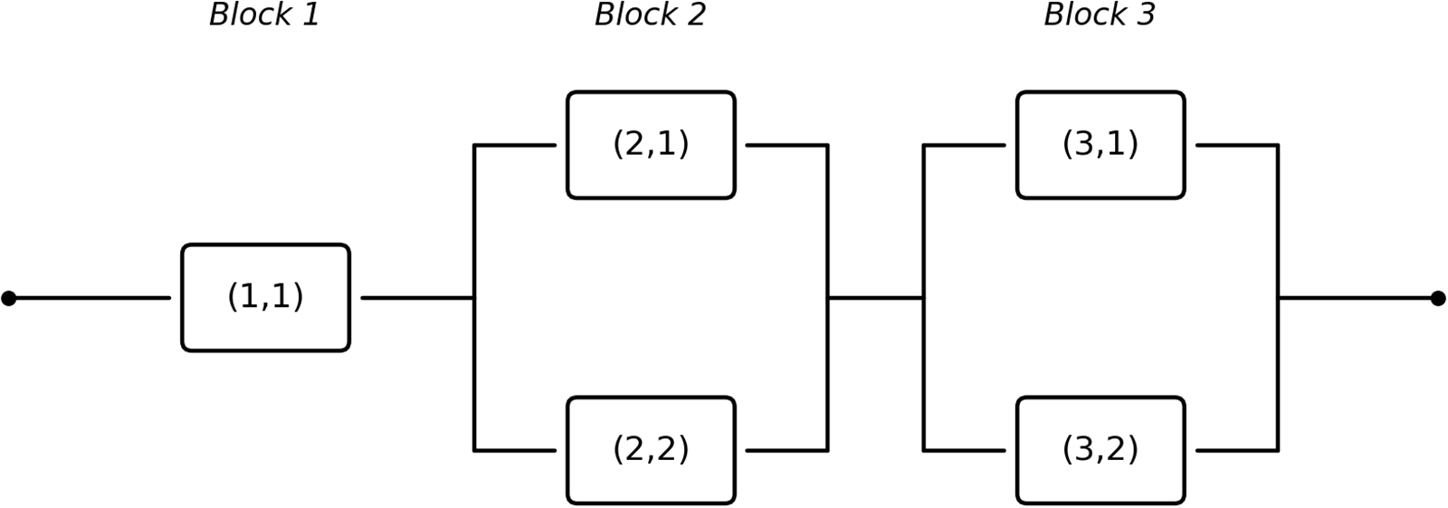
To fix ideas, we read the three-block example as a small power-supply system, of the kind found in the power networks mentioned in Section 1. The system has three stages in series: an intake stage, a conversion stage, and a distribution stage. The whole chain must work for the system to work, which gives the series structure. Stage 1 has a single unit, and stages 2 and 3 each have two redundant units in parallel, so  $\boldsymbol{n}=(1,2,2)$.
The shocks are voltage and thermal transients. Each unit faces its own local transients from its own load, which is the private source  $(i,j)$. The units in a stage also share a stage-wide stressor, such as transients on the common busbar or heat in the shared enclosure. This is the block-common source
 $(i,C)$, and it hits every unit in the stage at the same time. A unit withstands an isolated transient, but a run of
 $k$ consecutive severe transients damages it. This is the run mechanism, with
 $k=2$ here. The Erlang-2 interarrival times describe transients that arrive in a fairly regular pattern, less erratic than a Poisson stream.
The results then have a direct reading. The system MTTF is  $14.10$ time units with the shared transients and
 $27.19$ without them (Table 6), so a model that ignores the stage-wide stressor overestimates the life of the system by about a factor of two. For maintenance, Corollary 5.1 says that, to update the residual-life estimate of one unit, the operator needs only the latest inspection time among the other units in the same stage, not the full inspection history. This keeps condition-based inspection simple.
The model parameters can be estimated from field records. The transient arrival rates  $\lambda_r$ and the critical probabilities
 $p_r$ follow from event logs and severity thresholds, and phase-type fitting can match the interarrival distribution. A full calibration to a specific data set is left for future work.
6.2. System configuration and parameters
The Erlang $(2,\lambda)$ distribution has phase-type representation
 $\mathrm{PH}_c(\alpha,A)$ with
 $d=2$,
 $\alpha=(0,1)$, and
 $A=\bigl(\begin{smallmatrix}-\lambda&0\\\lambda&-\lambda\end{smallmatrix}\bigr)$; its mean is
 $2/\lambda$. We use the Erlang-2 distribution because it is the simplest phase-type distribution beyond the exponential. It has only two phases, which keeps the matrices small and the example easy to follow, while still exercising the full construction. Unlike the exponential, it is not memoryless and has an increasing hazard rate, so it describes shock interarrivals that are more regular than a Poisson stream. The method itself works for any phase-type interarrival distribution, and Erlang-2 is used here only as a transparent illustration. Table 2 gives the rate and critical probability for each of the eight shock sources; the run-length threshold is
 $k=2$ throughout. Figure 2 shows the system architecture.
Erlang-2 rate parameters and critical shock probabilities.

Table 2 Long description
Columns are Block, Source, Rate lambda r, and p r. Block 1 lists Private (1,1) with rate 0.5 and p r 0.30, and Block-common (1,C) with rate 0.9 and p r 0.25. Block 2 lists Private (2,1) with rate 0.6 and p r 0.35, Private (2,2) with rate 0.8 and p r 0.30, and Block-common (2,C) with rate 1.0 and p r 0.20. Block 3 lists Private (3,1) with rate 0.4 and p r 0.40, Private (3,2) with rate 0.7 and p r 0.25, and Block-common (3,C) with rate 1.2 and p r 0.15. Across blocks, Block-common rates increase from 0.9 to 1.0 to 1.2 while their p r values decrease from 0.25 to 0.20 to 0.15. Private sources span rates from 0.4 to 0.8 and p r values from 0.25 to 0.40.
Three-block series–parallel system,  $\boldsymbol{n}=(1,2,2)$.

6.3. Phase-type representations and state-space dimensions
Applying Proposition 3.1 to each source gives  $\bar{d}_r = d_r k = 2\times 2 = 4$ for all eight sources. Theorems 4.1–4.3 then yield the dimensions shown in Table 3.
State-space dimensions at each hierarchical level.

Table 3 Long description
Hierarchical levels list a quantity and its state space dimension. Run shock time uses Tr2 for each source with dimension 4. Component level lists Sij for all components with dimension 16. Intermediate maxima list W2 as the maximum of T21 and T22 with dimension 24, and W3 as the maximum of T31 and T32 with dimension 24. Block level lists S1 with n1 1 and dimension 16, S2 with n2 2 and dimension 96, and S3 with n3 2 and dimension 96. System level lists T as the minimum of S1, S2, and S3 with dimension 147,456.
The system parameters are  $\alpha_{\mathrm{sys}}=\alpha^{(1)}\otimes\alpha^{(2)}\otimes\alpha^{(3)}
\in\mathbb{R}^{1\times147456}$ and
 $A_{\mathrm{sys}}=A^{(1)}\oplus A^{(2)}\oplus A^{(3)}
\in\mathbb{R}^{147456\times147456}$. All subsequent computations exploit the Kronecker factorization
 $\exp(A_{\mathrm{sys}}t)=\exp(A^{(1)}t)\otimes\exp(A^{(2)}t)
\otimes\exp(A^{(3)}t)$, replacing one enormous matrix exponential with three small ones (Remark 4.2). All calculations were performed in MATLAB.
6.4. Reliability measures
Table 4 reports MTTF values at all levels.
Mean time to failure at component, block, and system level.

Table 4 Long description
Mean time to failure is listed in time units for each entity in the column labeled, MTTF time units. Component 1,1 is 26.7221; Component 2,1 is 24.1004; Component 2,2 is 23.6682; Component 3,1 is 30.4329; Component 3,2 is 35.3844. Block 1 is 26.7221, Block 2 is 32.0006, and Block 3 is 44.4071. System T is 14.1001.
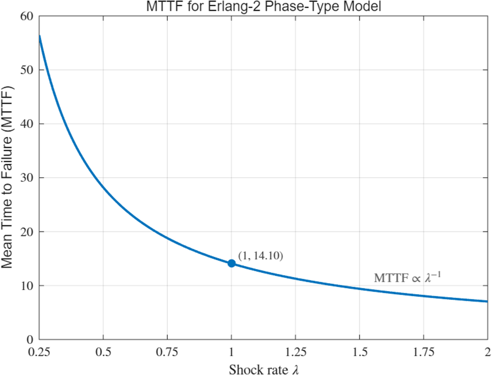
Parallel redundancy raises the block MTTF above any individual component MTTF (e.g.,  $\mathbb{E}[S_2]=32.00 \gt 24.10=\mathbb{E}[S_{21}]$), while the series connection reduces the system MTTF well below any block MTTF. Block 1, with a single component, is the reliability bottleneck. Figure 3 shows MTTF as a function of a common shock rate scale factor
 $\lambda$.
System MTTF as a function of shock rate scale factor  $\lambda$. The approximately hyperbolic decay is consistent with the
 $\mathrm{MTTF}\propto\lambda^{-1}$ scaling of PH distributions.

6.5. Sensitivity analysis
Table 5 consolidates the most informative parameter variations: run-length threshold  $k$, common critical probability
 $p$ (all sources set equal), and block size configuration.
System MTTF and state-space dimension under key parameter variations (baseline =  $k=2$, heterogeneous
 $p_r$ from Table 2,
 $\boldsymbol{n}=(1,2,2)$).

Table 5 Long description
Columns list varied parameter, value, mean time to failure, and system state space dimension. For run length, mean time to failure is 2.77 at 1, 14.10 at 2, 53.56 at 3, and 193.70 at 4; the system state space dimension is 1 024, 147 456, 2 985 984, and 26 214 400 for those same values. For critical probability with all sources equal, mean time to failure is 58.97 at 0.10, 17.43 at 0.20, 9.25 at 0.30, 6.20 at 0.40, and 4.68 at 0.50; the system state space dimension is not shown for these rows. For configuration n, mean time to failure is 11.02 for (1,1,1), 14.10 for (1,2,2), 15.74 for (2,2,2), 17.28 for (2,3,3), and 17.84 for (3,3,3). In the configuration section, the system state space dimension is shown only for (1,2,2) as 147 456, and is not shown for the other configurations.
Three conclusions emerge from Table 5. Increasing  $k$ yields the largest MTTF gains (a factor of
 $\sim70$ from
 $k=1$ to
 $k=4$) at the cost of rapidly growing state-space dimension, which scales as
 $O(k^{2m})$. The critical probability
 $p$ has a strongly non-linear effect: halving
 $p$ from 0.4 to 0.2 almost triples the MTTF. Parallel redundancy shows sharply diminishing returns: the first redundant component per block provides the largest improvement, with successive additions yielding progressively smaller gains.
6.6. Comparison with independent failure model
In the independent failure model, block-common shocks are absent and each component fails solely due to its private source:  $S_{ij}^{\mathrm{ind}}=T_{ij}(k)$. Table 6 compares key metrics.
Marshall–Olkin (MO) model vs. independent failure (IND) model.

Table 6 Long description
Metrics are listed in rows, with two columns of values labeled, MO model and IND model. For expected S one one, MO model is 26.72 and IND model is 57.78. For expected S two one, MO model is 24.10 and IND model is 36.73, and for expected S two two, MO model is 23.67 and IND model is 36.11. For expected S one, MO model is 26.72 and IND model is 57.78, and for expected S two, MO model is 32.00 and IND model is 53.13. For expected T, MO model is 14.10 and IND model is 27.19.
The MO model yields a system MTTF 48% lower than the independent model. Ignoring block-common shocks produces severely over-optimistic reliability predictions, which could lead to inadequate safety margins in engineering design.
6.7. Conditional MRL within block 2
We apply Theorem 5.1 to Block 2 ( $n_2=2$), so
 $t^{-}=t_2$, using the parameters from Table 2 with
 $k=2$. Three reference quantities bracket the conditional MRL family: (i) the marginal MRL
 $E(S_{21}-t_1\mid S_{21} \gt t_1)$ at
 $t_1=0$ equals
 $E[S_{21}]=24.10$ time units; (ii) the private-source MRL
 $E(T_{21}(2)-t_1\mid T_{21}(2) \gt t_1)$ at
 $t_1=0$ equals
 $E[T_{21}(2)]=36.73$ time units—the upper envelope approached as
 $t^{-}\to\infty$; (iii) the conditional MRL for
 $t_1\geq t^{-}$ (Case 1) coincides exactly with the marginal MRL.
Table 7 reports conditional MRL values at  $t_1=0$ for selected
 $t^{-}$.
Conditional MRL of component  $(2,1)$ at
 $t_1=0$ for selected observation times
 $t^{-}$ of component
 $(2,2)$.
 $k=2$; parameters from Table 2.

Table 7 Long description
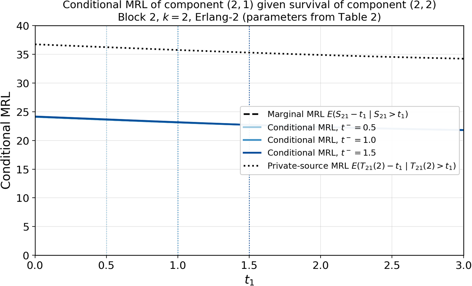
Mean residual life values are listed in time units for several quantities, alongside an observation time labeled t minus. The marginal mean residual life for S21 is 24.1004. The conditional mean residual life for S21 given S22 exceeds t minus is 24.1021 at t minus 0.5, 24.1186 at t minus 1.0, and 24.1643 at t minus 1.5. The private source mean residual life for T21 with 2 in parentheses is 36.7347 at t minus infinity.
Figure 4 displays the full conditional MRL curves over  $t_1\in[0,3]$ for
 $t^{-}\in\{0.5,1.0,1.5\}$, together with the marginal MRL (dashed) and the private-source MRL (dotted upper envelope).
Conditional MRL of component  $(2,1)$ given
 $S_{22} \gt t^{-}$, for
 $t^{-}\in\{0.5,1.0,1.5\}$ (solid curves, increasing shade). Dashed: marginal MRL. Dotted: private-source MRL (upper envelope). Vertical dotted lines: case boundaries
 $t_1=t^{-}$. Block 2,
 $k=2$.

Four key observations follow. First, the conditional MRL is strictly increasing in  $t^{-}$ for fixed
 $t_1 \lt t^{-}$, confirming Corollary 5.1: a later companion observation implies stronger deferral of the block-common shock and uniformly improves the residual life outlook for component
 $(2,1)$. Second, each conditional curve merges exactly with the marginal MRL at
 $t_1=t^{-}$ and remains coincident for
 $t_1 \gt t^{-}$, visually confirming Remark 5.2. Third, the conditioning effect at
 $t_1=0$ is modest (increments of 0.002, 0.018, 0.064 time units for
 $t^{-}=0.5,1.0,1.5$), because the low block-common probability
 $p_{2C}=0.20$ makes
 $E[T_{2C}(2)]=60$ time units far exceed the private mean
 $E[T_{21}(2)]=36.73$; in systems where the common shock is the dominant failure mechanism, the conditioning effect would be substantially larger. Fourth, the private-source MRL of 36.73 lies 12.63 time units above the marginal MRL of 24.10, measuring the total contribution of the block-common shock to the failure risk: without it, component
 $(2,1)$ would be expected to survive 52% longer.
6.8. Monte Carlo validation
We validate the analytical results by direct Monte Carlo simulation. For each shock source we draw the interarrival times as  $\mathrm{Erlang}(2,\lambda_r)$ and mark each shock as critical with probability
 $p_r$. The run-shock time
 $T_r(k)$ is recorded at the first run of
 $k$ consecutive critical shocks. The component, block, and system lifetimes are then obtained from
 $S_{ij}=\min(T_{ij}(k),T_{iC}(k))$,
 $S_i=\max_j S_{ij}$, and
 $T=\min_i S_i$. We use
 $N=4\times 10^{6}$ independent replications with the parameters of Table 2 and
 $k=2$. Table 8 compares the analytical MTTF values of Table 4 with the simulated means, the half-width of the
 $95\%$ confidence interval, and the relative error.
Analytical MTTF (Theorems 4.1–4.3) versus Monte Carlo estimates ( $N=4\times 10^{6}$ replications).

Table 8 Long description
Entities are listed with two columns of values labeled, Analytic and, MC mean. Component 1,1 has 26.7221 analytic and 26.7116 MC mean. Component 2,1 has 24.1004 and 24.0891, and Component 2,2 has 23.6682 and 23.6620. Component 3,1 has 30.4329 and 30.4169, and Component 3,2 has 35.3844 and 35.3857. Block 1 has 26.7221 and 26.7116, Block 2 has 32.0006 and 31.9963, and Block 3 has 44.4071 and 44.4111. System T has 14.1001 analytic and 14.0965 MC mean.
The conditional MRL values of Table 7 were reproduced in the same way: at  $t_1=0$, the simulated
 $E(S_{21}\mid S_{22} \gt t^{-})$ is
 $24.09$,
 $24.11$, and
 $24.15$ for
 $t^{-}=0.5,1.0,1.5$, against the analytical
 $24.10$,
 $24.12$, and
 $24.16$.
The comparison also illustrates the cost of the two approaches. The matrix-exponential method returns the exact values from small block matrices in a fraction of a second. Direct simulation needs several million replications to reach two-decimal accuracy and still leaves a sampling error. The two methods agree, but the analytical method is exact and much cheaper for the same accuracy.
7. Conclusion
This paper has resolved a fundamental obstacle in extending the MO run shock model of [Reference Ozkut and Eryilmaz21] from two-component systems to general  $m$-block series–parallel architectures. The obstacle is that component lifetimes within a parallel block are dependent through the shared block-common run-shock time
 $T_{iC}(k)$. This dependence blocks the direct use of the phase-type maximum closure. We removed it with Lemma 4.1, which establishes the representation
 $S_i=\min(T_{iC}(k),\max_j T_{ij}(k))$ and thereby re-expresses the block lifetime in terms of mutually independent random variables. Building on this lemma, Theorems 4.2–4.3 construct exact phase-type representations for block and system lifetimes via nested Kronecker product operations, and Theorem 4.4 provides closed-form dimension formulas quantifying how state-space complexity scales with system size, phase dimensions, and the run-length threshold
 $k$. A second independent contribution, Theorem 5.1, derives closed matrix-exponential formulas for the conditional mean residual life of any component given survival observations of its block companions; Corollary 5.1 establishes the structural invariance property that the result depends on those observations only through their maximum—a property specific to the MO parallel-block architecture with no counterpart in independent-failure models.
We note what is new here relative to the existing literature. Lemma 4.1 does not appear in the two-component model of [Reference Ozkut and Eryilmaz21], where the lifetimes are independent, and the maximum closure is not needed. It is the step that makes the hierarchical construction work for blocks with more than one component. The conditional MRL invariance of Corollary 5.1 is, to our knowledge, also new: the survival observations of the other components in a block affect the conditional MRL of a given component only through their maximum, whatever the number of components and their phase-type parameters. As shown in Section 6.1, this gives a simple rule for condition-based maintenance.
The three-block numerical illustration ( $m=3$,
 $\boldsymbol{n}=(1,2,2)$, Erlang-2 interarrival times,
 $k=2$) yields a system MTTF of 14.10 time units, compared with 27.19 under the independent failure model—a reduction of 48%, showing that ignoring block-common shocks produces severely over-optimistic predictions. Increasing
 $k$ from 1 to 4 raises the MTTF by a factor of 70 at the cost of a state-space dimension growing from
 $1\,024$ to over
 $26$ million, while halving the critical probability from 0.4 to 0.2 nearly triples the MTTF. For the conditional MRL within Block 2, the private-source mean of 36.73 time units exceeds the marginal mean of 24.10 by 12.63 time units, quantifying the total contribution of the block-common shock to component failure risk; the conditioning effect grows monotonically with the companion observation time
 $t^{-}$, consistent with Corollary 5.1.
The model has three principal limitations. First, the run-length threshold  $k$ is assumed common to all shock sources; allowing source-specific thresholds
 $k_r$ is conceptually straightforward but requires re-deriving the geometric-order distribution at each source. Second, the phase-type class requires finite-support interarrival distributions; systems with heavy-tailed shock interarrivals would require matrix-exponential approximations with attendant truncation error. Third, the framework is restricted to series–parallel topologies; extension to general coherent systems or
 $k$-out-of-
 $n$ blocks would require replacing the min/max closure pipeline with a more general reliability-function decomposition.
Three concrete extensions emerge naturally from the present work. (i) Source-specific thresholds: allowing  $k_r$ to vary by source would capture heterogeneous component resilience and require only localized changes to Proposition 3.1 and Lemma 4.1. (ii) Optimal inspection scheduling: the conditional MRL invariance in Corollary 5.1 directly motivates a maintenance optimization problem in which inspection times
 $t_1,\ldots,t_{n_i}$ are chosen to maximize or bound the conditional residual life of the most critical component, exploiting the reduction to the scalar
 $t^{-}$ to make the problem analytically tractable. (iii) Shock–degradation interaction: combining the run shock mechanism with a cumulative degradation process (Wiener or gamma process) at each component would produce a competing-risks model capturing both sudden-failure and wear-out mechanisms within the same Kronecker algebraic framework.
Acknowledgements
The authors would like to thank the Editor and the four referees for their careful reading of the manuscript and for their valuable suggestions, which helped improve both the presentation and the content of the paper.
Funding statement
This study was supported by the Scientific and Technological Research Council of Türkiye (TÜBİTAK) under the 2209-A University Students Research Projects Support Program (Project No: 1919B012530292).
Competing interest
The authors have no competing interests to declare.










 Open access

