1. Introduction
1.1. Motivations
Beam-plasma interactions are nowadays receiving some considerable renewed interest especially in the relatively unexplored regimes of high beam intensities and high plasma densities. One particular motivation lies in the fast ignition schemes (FIS) for inertial confinement fusion (Tabak et al., Reference Tabak, Hammer, Glinsky, Kruer, Wilks, Woodworth, Campbell, Perry and Mason1994; Deutsch et al., Reference Deutsch, Furukawa, Mima, Murakami and Nishihara1996, Reference Deutsch, Furukawa, Mima, Murakami and Nishihara1997). These should involve in their final stage the interaction of an ignition beam composed of MeV electrons laser generated at the critical density surface with a dense plasma target. The exploration of the electron beam transport into the overdense plasma is essential to assess the efficiency of the beam energy deposit. In this matter, transverse beam-plasma instabilities could be particularly deleterious in preventing conditions for burn to be met. Related theoretical studies have been mostly devoted to the linear regime of instabilities originating from current and charge neutralized equilibria (See e.g., Bret et al., Reference Bret, Firpo and Deutsch2004, Reference Bret, Firpo and Deutsch2005a, Reference Bret, Firpo and Deutsch2005b, Reference Bret, Firpo and Deutsch2005c, Reference Bret, Firpo and Deutsch2007, Reference Bret, Gremillet, Benisti and Lefebvre2008). However, one may argue that the physics of the fast ignition is intrinsically out-of-equilibrium. This was the motivation to consider in (Firpo et al., Reference Firpo, Lifschitz, Lefebvre and Deutsch2006) the out-of-equilibrium initial value dynamical problem taking place when a radially inhomogeneous electron forward current is launched into a plasma. The aim of this article is to tackle this problem in a rigorous and detailed way in order to obtain a precise picture of the early-time electromagnetic fields produced. Apart from the general inertial fusion and FIS contexts, discussed respectively by Deutsch Reference Deutsch2004; Hoffmann et al., Reference Hoffmann, Blazevic, Ni, Rosmej., Roth, Tahir, Tauschwitz, Udrea, Varentsov, Weyrich and Maron2005; Deutsch et al., Reference Deutsch, Bret, Firpo, Gremillet, Lefebvre and Lifschitz2008; Norreys et al., Reference Norreys, Beg, Sentoku, Silva, Smith and Trines2009, this study should be interesting to general physics research studies involving the propagation of a charged particle beam into a plasma such as the very active field of plasma-based accelerators (See Esarey et al., Reference Esarey, Schroeder and Leemans2009; Kumar et al., Reference Kumar, Pukhov and Lotov2010). Interestingly enough, the apparently purely academic case of an electron beam with sharp edges considered here happens moreover to be truly relevant to model electron beams constrained to move along a wire. For instance, the recent study presented in Green et al. (Reference Green, Lancaster, Akli, Gregory, Beg, Chen, Clark, Freeman, Hawkes, Hernandez-Gomez, Habara, Heathcote, Hey, Highbarger, Key, Kodama, Krushelnick, Musgrave, Nakamura, Nakatsutsumi, Patel, Stephens, Storm, Tampo, Theobald, Van Woerkom, Weber, Wei, Woolsey and Norreys2007) involves an experimental implementation of a wire plasma that may be relevant to fast-ignition inertial fusion.
1.2. Framework
The physical system considered is that of a radially inhomogeneous electron forward current launched at an initial time into a plasma with no initial current compensation. The direction of the beam is along the z-axis. This study will be devoted to the extreme case where the beam is cylindrical with sharp edges so that the current may be written

where H denotes the Heaviside function. The focus is put on this early stage where collisions may be neglected. Ions will be assumed to form a fixed neutralizing background. In order to simplify the analysis, the system is taken to be invariant along the beam direction, z (Firpo et al., Reference Firpo, Lifschitz, Lefebvre and Deutsch2006; Taguchi et al., Reference Taguchi, Antonsen, Liu and Mima2001; Firpo & Lifschitz, Reference Firpo and Lifschitz2007). The plasma density n p will be taken as uniform and constant.
Maxwell equations in cylindrical coordinates read
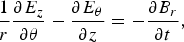
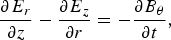






where the beam current jb acts as a given source term. Provided that the density of plasma electrons, that are initially at rest, is much larger that the density of beam electrons, the electron plasma current jp = −en pvp is given by linear fluid theory in some initial transient stage, so that
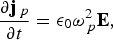
with ωp2 = n pe 2/(m eε0). The Reader is referred to the Appendix sections A and B for a detailed derivation of Eq. (10) as well as for a discussion on its validity domain.
We Fourier decompose any field g(r, θ ,z, t) through

After manipulating Eqs. (2)–(7), in order to express the electric field components as functions of the magnetic field components, one is left with a single wave equation for the magnetic field on m = 0, namely one has to solve, for t > 0,
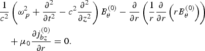
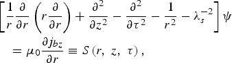
We focus here on the rotationally invariant part of the magnetic field. The m ≠ 0 components, that are initially vanishing, would only become non-zero as a result of a possible beam-plasma instability that may appear in a later stage. Putting τ = ct and introducing the electron skin depth λs = c/ωp, (Eq. (11)), that is to be solved for t > 0, reads
with ψ ≡ B θ(0) for j bz given by (1).
2. Calculation of the poloidal magnetic field: The Laplace transform's approach
Eq. (12) may be further simplified by introducing the reduced radial variable  , the dimensionless variables
 and ratio η ≡ r b/λs. It reads then

This dimensionless system will be used in this Section. For the sake of clarity, we shall drop the tildes writing, from now on in this Section, r, z, τ and ψ in place of  and
 . Let us now proceed to a Laplace transform in time of Eq. (13) and define

Taking into account the invariance of the problem along z, one is left with

The Green function g(r | a) Duffy (Reference Duffy2001) solving ℒ1g = −δ(r − a) is readily computed as  with r < = min(r, a) and r > = max(r, a). The solution of Eq. (14) is then

This must be Laplace inverted to obtain the solution in the real time space. From this expression, let us note that it would be possible to obtain the radial behavior of an approximate solution to our problem in separated time-space variables, valid at large enough times, by using that  (See Kuppers et al., Reference Kuppers, Salat and Wimmel1973; Firpo et al., Reference Firpo, Lifschitz, Lefebvre and Deutsch2006). That this would be only an approximate solution will become explicit in Section 3. However, this enables to estimate the large time behavior of the m = 0 component of the poloidal magnetic field for large values of η using, for x ≫ 1,


One obtains
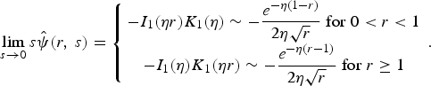
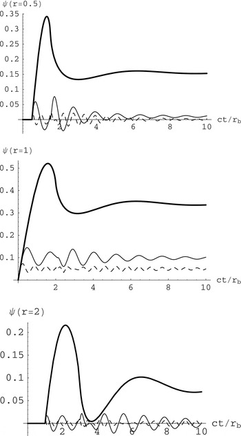
Therefore, except in the vicinity of the border of the beam (for r ≃ 1), the magnetic field decreases strongly when the ratio η becomes large, which will be apparent on Figure 1.
Initial time behavior of the m = 0 component of the poloidal magnetic field for three different values of η, namely η = 1 (bold), η = 5 (plain), and η = 10 (dashed line) at different radius: r = 0.5 (upper plot), r = 1 (middle plot), and r = 2 (bottom plot).

The problem of the analytical obtention of B θ(0) (r, t) = ψ(r, t) will be addressed in the following section using an alternative approach. Here we shall present results coming from numerical Laplace inversions of Eq. (15). Figure 1 presents the time evolution of the axisymmetric component of the poloidal magnetic field measured at three different radii, namely at r = 0.5, r = 1, and r = 2, for three values of η. Curves have been obtained using a Gaver-Wynn-Rho algorithm for Laplace transform's inversion presented by Valkó and Abate (Reference Valkó and Abate2004).
3. Calculation of the poloidal magnetic field: The Riemann's method
3.1. Implementation of Riemann's method
In this Section, the problem will be addressed through a Hankel transform in the radial variable followed by the use of Riemann's method for hyperbolic differential equations in the two independent variables z and τ. In this respect, the present study follows the line of approach pursued in particular in several papers by Borisov and Simonenko (Reference Borisov and Simonenko1994) and Borisov (Reference Borisov2002).
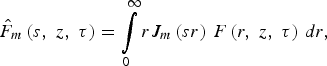
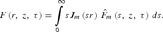
The Fourier-Bessel transform, also called Hankel transform, of order m of some function F is defined by
while its inverse transform is obtained through
Applying the Hankel transform of order 1 to Eq. (12) yields

3.2. First possible expression for the solution
The Riemann function R of the equation

may be written, by the virtue of Olevsky's theorem (See Borisov (Reference Borisov2002), Olevsky (Reference Olevsky1952), as the following sum of terms
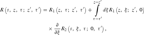
where  is the Riemann function of Eq. (20) taking s = 0 and
 is the Riemann function of Eq. (20) taking λs−1 = 0. Eq. (21) reads then
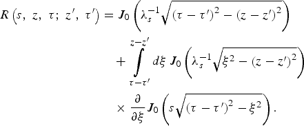
Using Riemann's formula, the solution of Eq. (19) reads

It remains to inverse Hankel transform through
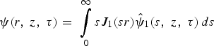
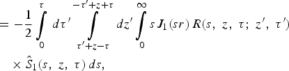
where one has used
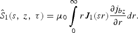
The definition of the beam current given in Eq. (1) gives

which yields

Eq. (23) becomes
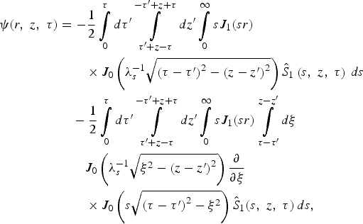
that is

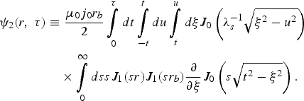
with τ > 0. The expressions of the two contributions in Eq. (24) may be simplified since, as expected, they may be put in a form explicitly independent on z when moving from variables τ′ and z′ to variables t = τ− τ′ and u = z − z′. This yields
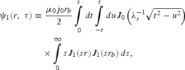
Let us begin with the calculation of ψ1. Using Gradshteyn and Ryzhik (Reference Gradshteyn and Ryzhik2007),
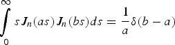
gives

The integral

is evaluated using the identity

This yields

Using then ∫0XxJ −1/2 (x) J 1/2 (x) dx = sin2X/π finally gives
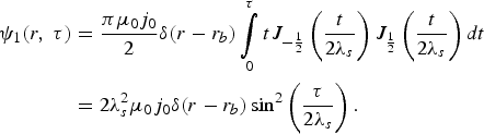
This is just

The second contribution to the field involves an integral of a triple product of Bessel functions of the type

for r, r b, α > 0, through which causality relations will come into play. From Gradshteyn and Ryzhik (Reference Gradshteyn and Ryzhik2007), this yields

where P 1/21/2 (.) is the Legendre function of the first kind, and the angle v satisfies

and

It happens that the expression of  (r,r b,α), as written in Gradshteyn and Ryzhik (Reference Gradshteyn and Ryzhik2007), should be completed by the singular special case
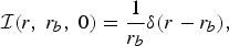
due to Eq. (27). Let us consider now this second component of the poloidal magnetic field
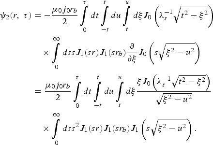
Putting 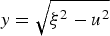 , it comes
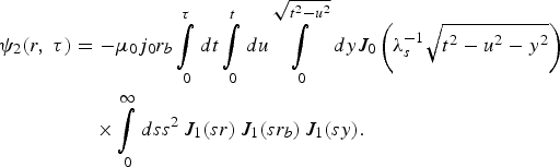
We have to compute, from Eq. (29),

Let us integrate  by part. Eq. (31) yields
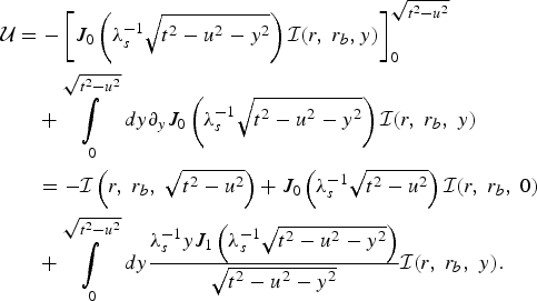
The second term in this last expression will yield the opposite of the singular term obtained for ψ1 in Eq. (28), ensuring thereby the regularity of the field. We are thus left with
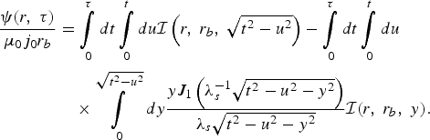
Eq. (32) may have been obtained more directly by using Olevsky's theorem interchanging R 1 and R 2 in Eq. (21). The former decomposition was amenable to a — relatively — easy estimation of the “purely plasma” component ψ1(r, τ) leading to a singular solution with time and space separated. This singular part of the solution was however canceled in ψ2(r, τ). Eq. (32), that decomposes into two integrals involving  , expresses in particular the fact that an exact solution in separated variables, time and space, cannot exist. The relevant decomposition (32) shows that the poloidal magnetic field component is the superposition of a “purely vacuum” term

and of a term involving the plasma contribution
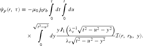
3.3. Solution decomposing into a vacuum and a plasma parts
Section 3.2 eventually turned into a sort of pedagogically digression. The interchangeability between R 1 and R 2 in Eq. (21) appears as a fake one and one is left with the need to estimate the vacuum contribution (33) and the plasma contribution (34).
3.3.1. Vacuum Contribution
Let us first estimate ψv(r, τ). We have
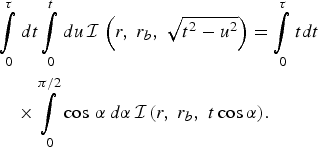
Let us evaluate

with

and where the definition domain  of the integral is given by the condition |r − r b| < t cos α < r + r b. Three cases are to be considered: If t ≤ |r − r b|, then
 , from which it will follow that ψv = 0 for τ ≤ | r − r b|. If |r − r b| < t and r + r b > t, then
 = [0; arccos (| r − r b|/t)]. Finally, if r + r b ≤ t, then
 . A change of variables yields

where  is the definition domain of the integral in the v variable. The last integral is defined provided that cos v + a > 0, where a is given by a(r, r b, t) ≡ (t 2 − r 2 − r b2)/(2rr b) and reads then

We shall use the primitive (See Gradshteyn and Ryzhik, Reference Gradshteyn and Ryzhik2007),

for |a| < 1 and 0 ≤ x < arccos(−a), with 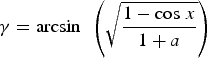 and
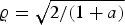 . Here E is the elliptic integral of the second kind
 and F the elliptic integral of the first kind
 . Consequently, in the time and space domain satisfying |r − r b| < t and r + r b > t, one will use Eq. (35) for the primitive. Using reduced (dimensionless) variables, one puts
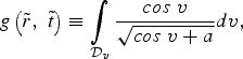
with, for  and
 ,

where E and K denote, respectively, the complete elliptic integral of the second and first kind, and elsewhere, namely for  or


Finally, the vacuum contribution to the poloidal magnetic field is obtained as a time integral of g, namely through

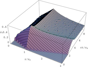
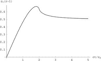
Figure 2 represents the evaluation of  in the time-space domain whereas Figure 3 shows the comparison between the evaluation of the vacuum contribution of the poloidal magnetic field at the radius r = r b using Eq. (36) and its evaluation through the numerical Laplace transform inversion of Eqs. (15) for η = 0.
(Color online) Contribution of the vacuum to the poloidal magnetic field. The representation is given in non-dimensional variables.

 using expression (

3.3.2. Plasma Contribution
Let us now consider the plasma contribution to the poloidal magnetic field (34). The plasma contribution involves the double integral

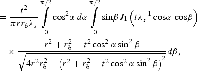
in which the product cosα sinβ is constrained by the condition |r − r b|/t < cosα sinβ < (r + r b)/t. Let us make the following change of variables: u = cos α cos β, v = cos α sin β. One gets
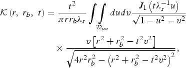
where the integration domain  is contained into the upper quarter of the unit circle. We can thus write
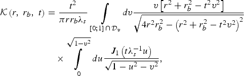
with ![${\cal D}_u \equiv ]\vert r - r_b \vert /t; (r + r_b)/t$](https://static.cambridge.org/binary/version/id/urn:cambridge.org:id:binary:20151021100151072-0360:S0263034612000432_inline26.gif?pub-status=live) [. However, we have, using Eq. (6.552) in Gradshteyn and Ryzhik (Reference Gradshteyn and Ryzhik2007),
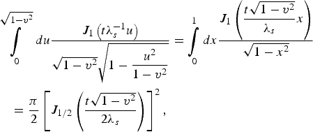
so that
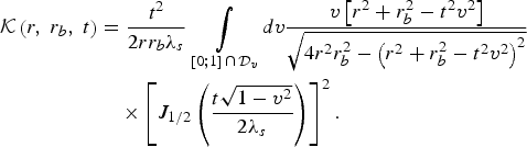
In terms of the dimensionless variables introduced in Section 2, we are left with
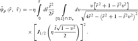
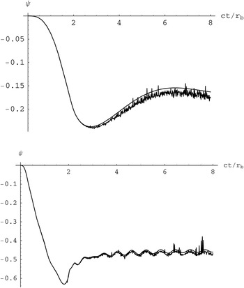
Figure 4 illustrates the time behavior of the plasma contribution to the poloidal magnetic field at some given radii and compares it to the one obtained from the Laplace inversion approach.
Time behavior of the “plasma” contribution to the poloidal magnetic field at r = r b for η = 1 (upper plot) and η = 10 (bottom plot). The smooth curves come from the numerical Laplace inverse transform of the full solution given in Eq. (15) subtracted from the vacuum solution (See Fig. 3). The curves showing some numerical noise have been obtained from the numerical evaluation of Eq. (37). The representation is given in non-dimensional variables.

3.3.3. The Full Solution
One can now proceed to the computation of the full poloidal magnetic field by summing the so-called vacuum (36) and plasma (37) contributions. The time-space representation of the poloidal magnetic field in non-dimensional coordinates is plotted in Figure 5. In the limit η → ∞, one can check that the poloidal magnetic field vanishes, meaning that the plasma contribution compensates exactly the vacuum one. This is in agreement with the asymptotes obtained in the large η limit in Eq. (18). Therefore, the most interesting behavior takes place for intermediary values of η, namely for values of the beam radius of the order of some electron skin depths. The (m = 0 component of the) poloidal magnetic field is first created in the initial stage that looks like a choc. In the vacuum limit η → 0, the poloidal magnetic field quickly tends to a steady value after this initial choc stage. For low values of η, it displays a transient intermediary stage showing a small number of wave-like variations that rapidly damp. When η gets larger, these plasma-like ripples last longer while their adimensional time period (in terms of ct/r b) decreases.
(Color online) Space and initial time evolution of the total poloidal magnetic field in terms of non-dimensional variables for η = 1 (left upper plot), η = 2 (right upper plot), η = 5 (left bottom plot) and η = 10 (right bottom plot).

4. Conclusion
In this article, a detailed computation of the poloidal magnetic field created by the sudden injection of an electron beam with sharp edges into a plasma has been presented. The control parameter of the problem appears to be η, namely the ratio of the beam radius to the electron skin depth. Two different ways to address analytically this problem have been considered. One way amounts to proceed to an inverse Laplace transform of a solution having a relatively simple expression, given in Eq. (15), in the reciprocal space. Another way involves the Riemann's method. This leads to some rather intricate calculations in which, e.g., causality conditions manifest through some integrals of triple products of Bessel functions. However one advantage of the later approach is to supply a formula that decomposes explicitly, thanks to Olevsky's theorem (Olevsky, Reference Olevsky1952), into a vacuum and a plasma contributions, a fact that follows from the linearity of the wave equation but that is not obvious to recover from the Laplace transform approach in Eq. (15). This decomposition provides an easy way to capture the space-time behavior of the poloidal magnetic field.
This study should hopefully provide a calculation useful to benchmark numerical codes or to develop analytical models.
Acknowledgments
The author is indebted to L. Gremillet for his critical comments on a preliminary version of this work. Useful discussions with A. Bret, C. Deutsch, and A.F. Lifschitz are gratefully acknowledged.
A. Linear plasma response
Let us consider the momentum equation for plasma electrons

in which P denotes a stress pressure tensor and ν an effective collision frequency.
At initial time, the plasma is at rest. The linear hypothesis consists in discarding the nonlinear convective term in the left hand side and the Lorentz force that are second order in vp. In particular, during the validity domain of the model, the plasma electrons are non-relativistic. In the present modeling, one neglects also the pressure tensor term, which amounts to a cold plasma hypothesis, and collisions. Together with the fluid equation of continuity
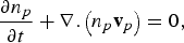
and using the definition of the electron plasma frequency

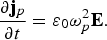
this yields, keeping only the first order terms in vp, the desired simple linear plasma response
B. Validity domain
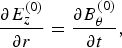
From Maxwell equations in cylindrical geometry, one obtains
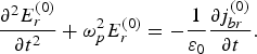
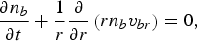
In order to estimate the source term in Eq. (40), one needs to compute j br(0). This requires to solve the fluid equations for the electron beam that read


Let us introduce the ratio α = n b0/n p. This will be assumed to be a small parameter. One can then expand the fields in terms of α and get n b = n b0 + αn b1, v br = αv br1, j br = αj br1 = −αen b0v br1. One obtains at first order
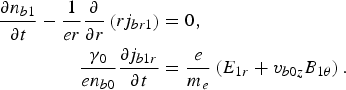
Therefore one has
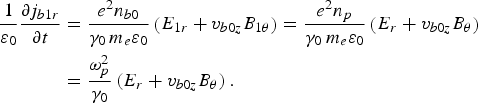
This yields

the solution of which reads
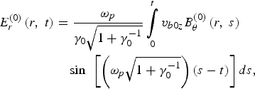
We have
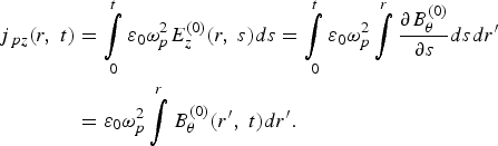
Therefore, by virtue of the fluid momentum equation for plasma electrons (38), the electrostatic description of plasma electrons is valid as long as the modulus of


is large in front of the modulus of
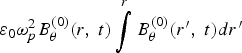

In the last Eqs. (42) and (44), one has used the dimensionless notation of Section 2. One has to evaluate the ratio

Whatever the value of η, one immediately see that κ remains large for a small α even if the numerator tends to cancel on times of the order of some ct/r b. When η becomes large, one can use the asymptotic behaviours written in Eq. (18). This ensures that κ remains large, since the denominator is of second order in an exponentially small quantity.