1. Introduction
The retina is a thin and multilayered neural tissue lining the back of the eye that plays a crucial role in visual function. Its function depends sensitively on adequate blood supply, as retinal haemodynamics helps sustain the metabolism that keeps the retina alive and functional (Kornfield & Newman Reference Kornfield and Newman2015). Disruptions in the haemodynamics can impair oxygen and nutrient delivery, contributing to various retinopathies such as diabetic retinopathy (Kornfield & Newman Reference Kornfield and Newman2015), glaucoma (Garhöfer et al. Reference Garhöfer, Zawinka, Resch, Huemer, Schmetterer and Dorner2004; Caprioli & Coleman Reference Caprioli and Coleman2010; Ch’ng et al. Reference Ch’ng, Chua, Ummi Kalsom, Azhany, Gong, Rasool and Liza-Sharmini2021) and retinal vascular occlusion (Osborne et al. Reference Osborne, Casson, Wood, Chidlow, Graham and Melena2004). Understanding retinal haemodynamics is thus essential for understanding the life of the retina in health and disease.
Computational modelling serves as a crucial and powerful tool for exploring the retinal haemodynamics, integrating physiological processes that are difficult to measure in vivo (Siggers & Ethier Reference Siggers and Ethier2012; Ruffini et al. Reference Ruffini, Dvoriashyna, Govetto, Romano and Repetto2024). Different models have been employed in retinal haemodynamics and oxygenation. Lumped parameter zero-dimensional (0-D) models, representing the vasculature as a hydraulic resistor circuit (Flores et al. Reference Flores, Alastruey and Corvera Poiré2016), have helped to resolve the inconsistencies in clinical data (Guidoboni et al. Reference Guidoboni, Harris, Cassani, Arciero, Siesky, Amireskandari, Tobe, Egan, Januleviciene and Park2014b ). The 0-D lumped model is also exploited in the simulation of retinal circulation (Ganesan et al. Reference Ganesan, He and Xu2010; Fry et al. Reference Fry, Coburn, Whiteman, Harris, Siesky and Arciero2018). More complicated models, including a one-dimensional (1-D) model, two-dimensional (2-D) model and three-dimensional (3-D) model, have been used to reveal fundamental properties of oxygen transport in the retina (Liu et al. Reference Liu, Wood, Witt, Hughes, Thom and Xu2009; Causin et al. Reference Causin, Guidoboni, Malgaroli, Sacco and Harris2016) as well as deal with properties of disease in specific patients (Malek et al. Reference Malek, Azar, Nasralli, Tekari, Kamoun and Tourki2015; Rebhan et al. Reference Rebhan, Parker, Kelsey, Chen and Doyle2019; Julien et al. Reference Julien, Bonnin, Paques and Fullana2023; Tripathy et al. Reference Tripathy, Siddharth and Bhandari2023). Existing models provide valuable physiological and pathological insights, however, they focus on specific vascular compartments, including simplifications such as constant capillary pressure or neglecting interactions between capillaries and surrounding tissue. Consequently, very few existing models combine the arterioles, venules, capillaries and tissue equally into a comprehensive model. In other tissues, the general rule that all compartments interact with each other has required a systematic structural analysis of flow (Eisenberg Reference Eisenberg2023), and the same should hold true for the retina.
A central challenge in modelling the haemodynamics of retinal microcirculation stems from intrinsic multiscale vasculature. Arteriolar and venular networks display hierarchical tree-like branching (Julien et al. Reference Julien, Bonnin, Paques and Fullana2023), while capillaries form an interconnected mesh-like structure (Fry et al. Reference Fry, Coburn, Whiteman, Harris, Siesky and Arciero2018; Shipley et al. Reference Shipley, Smith, Sweeney, Pries and Secomb2019). Thus, retinal microcirculation inherently constitutes a multiscale system, involving small-scale details of flow inside blood vessels and also the large-scale layout of the blood vessels. These issues can be addressed using existing methodologies for other organs or tissues, including tumour perfusion (d’Esposito et al. Reference d’Esposito2018), transport in breast tissue (Fritz et al. Reference Fritz, Köppl, Oden, Wagner, Wohlmuth and Wu2022) and microcirculatory haemodynamics (Shipley et al. Reference Shipley, Smith, Sweeney, Pries and Secomb2019; Sweeney et al. Reference Sweeney, Walsh, Walker-Samuel and Shipley2024), where a continuum Darcy model for capillary flow is typically coupled to arterial and venous trees via point sources. Even with the point source approximation, the computation is challenging because the Darcy model has to be solved simultaneously with arterial and venous flows (Qohar et al. Reference Qohar, Munthe-Kaas, Nordbotten and Hanson2021; Fritz et al. Reference Fritz, Köppl, Oden, Wagner, Wohlmuth and Wu2022). A novel alternative is to use the analytic solution for the capillary flow, which expresses the pressure explicitly so that the Darcy model does not have to be solved in the entire domain. The analytical solution provides significant physical insight as well as much faster computation (d’Esposito et al. Reference d’Esposito2018; Shipley et al. Reference Shipley, Smith, Sweeney, Pries and Secomb2019; Sweeney et al. Reference Sweeney, Walsh, Walker-Samuel and Shipley2024). However, in current analytic methods the fluid exchange between capillaries and tissue is treated approximately. They describe the coupling of capillaries between surrounding tissues using a far-field boundary condition. While this serves as a reasonable first step, it does not capture the local fluid exchange between these two components, and a more realistic description should include such exchange.
Our work complements previous studies by developing a novel multiscale model that fully couples retinal vasculature with interstitial tissue. Specifically, the flows in arterioles and venules are described by a 1-D model (Julien et al. Reference Julien, Bonnin, Paques and Fullana2023), while capillaries and surrounding tissue are treated as two coupled porous media and the flow in them is described by the Darcy equation. The fluid exchange between the capillary and tissue is modelled by the source/sink of the two Darcy equations, one for capillary (drainage) and the other for the tissue (feed). Moreover, the vasculature is coupled as follows. Terminal arterioles/venules in the superficial layer act as point sources/sinks in the capillary Darcy equation, and the pressure difference between these vessels and the capillary network is related to the flow rates at point sources/sinks by the effective resistors in the deep layer, which provides the outlet/inlet boundary condition for the arteriolar/venular tree in the superficial layer. What further distinguishes our modelling from others is the analytic solution for the capillary–tissue system, which is derived on a finite domain with physiological boundary conditions. We analyse the convergence and truncation error of the analytical solution extensively to ensure its robustness and accuracy. The analysis of the solution’s convergence also reveals some interesting properties, which might suggest a new modelling methodology for other tissues. The model is validated against experimental data and the results from existing models, and pulsatile pressures within arterioles and venules are also simulated. Moreover, we demonstrate our model’s capability by exploring the effects of parameter variations.
The rest of the paper is organised as follows. In § 2 we describe the models for vasculature and surrounding tissue, including the 1-D model for arterioles and venules, the synthetic vascular network model and the continuum formulation for the capillary–tissue system. In § 3, we derive the analytic solution of capillary–tissue coupled system, and its convergence is analysed. In § 4, the numerical methods for the proposed model are described, and multiple simulations are performed to assess the model’s accuracy and demonstrate its capability in § 5. The sensitivity of various parameters is explored in § 6. Section 7 consists of the conclusion and discussion.
2. Models
2.1. Network-based simulation for arteriolar and venular trees
2.1.1. One-dimensional model
The 1-D model is widely adopted to describe the blood flow in the individual vessels of arteriolar and venular networks. The networks exist in 3-D space but are often analysed in a 2-D subset of 3-D space following the usual conventions of electric circuit theory. For all time
 $t\gt 0$
, the flow within each vessel is characterised by the flow rate
 $q(s,t)$
and the cross-sectional area
 $A(s,t)$
(Wang et al. Reference Wang, Nishi, Matsukawa, Ghigo, Lagrée and Fullana2016; Julien et al. Reference Julien, Bonnin, Paques and Fullana2023), along the axis
 $s$
of the vessel, and their evolutions are given by
 \begin{eqnarray}\left \{ \begin{aligned} &\frac {\partial A}{\partial t}+\frac {\partial q}{\partial s}=0, \\[5pt] &\frac {\partial q}{\partial t}+\frac {\partial }{\partial s}\left (\hat {\alpha }\frac {q^2}{A}\right )+\frac {A}{\rho }\frac {\partial p}{\partial s}=C_{\!f}, \end{aligned}\right . \end{eqnarray}
where
 $\hat {\alpha }$
is the coefficient (momentum flux correction factor) that describes the velocity profile in each vessel (Müller & Toro Reference Müller and Toro2014),
 $p$
is the pressure,
 $\rho$
is the density of blood and
 $C_{\!f}$
is the friction term. The coefficient
 $\hat {\alpha }$
is set as
 $\hat {\alpha }=4/3$
, which corresponds to a parabolic velocity profile that is consistent with the experimental data in the retina (Song et al. Reference Song, Wei, Liu, Liu, Yi, Sheibani, Fawzi, Linsenmeier, Jiao and Zhang2014; Kornfield & Newman Reference Kornfield and Newman2015; Causin et al. Reference Causin, Guidoboni, Malgaroli, Sacco and Harris2016). The density is set as
 $\rho =1\,{\mathrm{g}\,\mathrm{cm}^{-3}}$
from now on in this paper. The explicit form of friction term is given by (Audebert et al. Reference Audebert, Bucur, Bekheit, Vibert, Vignon-Clementel and Gerbeau2017; Liu & Suito Reference Liu and Suito2024)
 \begin{eqnarray} C_{\!f}=\left \{\begin{aligned} &-8\pi \frac {\eta }{\rho }\frac {q}{A},\quad \text{for arterioles},\\[5pt] &-8\pi \sqrt {\frac {A}{A_0}}\frac {\eta }{\rho }\frac {q}{A},\quad \text{for venules}, \end{aligned}\right . \end{eqnarray}
where
 $\eta =\eta (r)$
is the apparent viscosity, modelled as a function of the vessel radius
 $r$
to account for the rheological properties of blood.
The fluid–structure interaction in the problem is captured by the following elastic model (Müller & Toro Reference Müller and Toro2014; Liu & Suito Reference Liu and Suito2024):
 \begin{eqnarray} p-p_{\textit{ext}}=K\left [\left (\frac {A}{A_0}\right )^{\beta _1}-\left (\frac {A}{A_0}\right )^{\beta _2}\right ]\!, \end{eqnarray}
where
 $p_{\textit{ext}}$
is the exterior pressure,
 $K$
is the rigidity,
 $\beta _1$
and
 $\beta _2$
are parameters depending on the vessel wall behaviour and
 $A_0$
is the neutral area of the vessel, which differs for each vessel. The values of
 $K$
,
 $\beta _1$
and
 $\beta _2$
vary with the vessel position and its function. The rigidity is
 \begin{eqnarray} K=\left \{\begin{aligned} &\frac {4}{3}\frac {\pi ^{1/2}Eh}{A^{1/2}_0}, \quad \text{for arterioles},\\[7pt] &\frac {1}{9}\frac {\pi ^{3/2}Eh^3}{A^{3/2}_0}, \quad \text{for venules}, \end{aligned}\right . \end{eqnarray}
where
 $E$
is the Young’s modulus and
 $h$
is the thickness of the vessel wall. The parameters
 $\beta _1$
and
 $\beta _2$
are given by
 \begin{eqnarray} \beta _1=\left \{\begin{aligned} &1/2,\quad \text{for arterioles},\\[3pt] &10,\quad \text{for venules}, \end{aligned}\right . \end{eqnarray}
and
 \begin{eqnarray} \beta _2=\left \{\begin{aligned} &0,\quad \text{for arterioles},\\[3pt] &-3/2,\quad \text{for venules}. \end{aligned}\right . \end{eqnarray}
The expression of
 $K$
and values of
 $\beta _1$
and
 $\beta _2$
for arterioles are mainly taken from previous work on modelling of arteriolar circulation (Julien et al. Reference Julien, Bonnin, Paques and Fullana2023), while those for venules are adopted from the model of veins in other tissues (Müller & Toro Reference Müller and Toro2014; Audebert et al. Reference Audebert, Bucur, Bekheit, Vibert, Vignon-Clementel and Gerbeau2017). The values of
 $E$
for arterioles and venules are set to the same value as a reasonable approximation (Julien et al. Reference Julien, Bonnin, Paques and Fullana2023). The wall thickness
 $h$
is proportional to the vessel diameter, which is given by
 $h=\mathrm{WLR}\times 2r_0$
, where
 $\mathrm{WLR}$
is the wall-to-lumen ratio and
 $r_0$
is the radius of neutral area
 $A_0$
. For arterioles, the value of
 $\mathrm{WLR}$
is based on experimental observations (Arichika et al. Reference Arichika, Uji, Ooto, Muraoka and Yoshimura2015), while for venules, a smaller value is employed to account for their thinner walls. Values of parameters in 1-D model are summarised in table 1.
Parameters for the haemodynamics in retinal microcirculation.

Table 1. Long description
The table presents parameters for a one-dimensional model of haemodynamics in retinal microcirculation. It includes three columns: Parameter, Value, and References. The table has 30 rows, each detailing specific parameters and their corresponding values and references. The parameters are grouped into categories such as Viscosity model, Elastic model, L-system, Structured tree model, Capillary-tissue coupled system, and Boundary conditions at CRA and CRV. Each row provides specific values and references for these parameters. The references include various studies and authors, providing a comprehensive overview of the sources used to derive these values.
The apparent viscosity of blood decreases strongly with the decreasing vessel radius from approximately 150 to approximately
 $5\,\mathrm{\unicode{x03BC} m}$
, then increases below
 $5\,\mathrm{\unicode{x03BC} m}$
. This unique rheological behaviour is the Fåhræus–Lindqvist effect. To characterise blood’s rheological properties, we use an empirical relation developed by Pries et al. that expresses viscosity as a function of vessel radius (Pries et al. Reference Pries, Secomb, Gessner, Sperandio, Gross and Gaehtgens1994; Secomb & Pries Reference Secomb and Pries2013; Bappoo et al. Reference Bappoo, Kelsey, Parker, Crough, Moran, Thomson, Holmes, Wyrwoll and Doyle2017)
 \begin{eqnarray} \eta (r)=\eta _p\left [1+(\eta _{45}-1)\left (\frac {r}{r-0.55}\right )^2\right ]\left (\frac {r}{r-0.55}\right )^2, \end{eqnarray}
where
 $r$
is the vessel radius (in unit
 $\mathrm{\unicode{x03BC} m}$
),
 $\eta _p$
is the viscosity of plasma set as
 $\eta _p=0.012\,\mathrm{Poise}$
and
 $\eta _{45}$
is the relative apparent blood viscosity for discharge haematocrit of
 $0.45$
given by
 \begin{eqnarray} \eta _{45}=6\exp (-0.17r)+3.2-2.44\exp \left [-0.06(2r)^{0.645}\right ]\!. \end{eqnarray}
Note that the 1-D model is adopted for superficial vessels, which are visible in fundus images. As a result, the external pressure acting on the vessel walls is approximately the intraocular pressure (IOP) (Kiel Reference Kiel2011), and thus in the 1-D model, external pressure is set to
 $p_{\textit{ext}}=\mathrm{IOP}$
. A similar approximation is employed in previous work (Guidoboni et al. Reference Guidoboni, Harris, Cassani, Arciero, Siesky, Amireskandari, Tobe, Egan, Januleviciene and Park2014b
). Smaller vessels are distributed in the deep layer and invisible in fundus images, which makes them difficult to distinguish clinically. The standard method is to model these deep vessels as effective resistors that connect the superficial vascular trees to the capillary bed. The synthetic vascular network model for both superficial and deep vessels is described below.
2.1.2. Synthetic vascular network model
Next, we construct a network from individual vessels. We exploit a Lindenmayer system (L-system) to generate synthetic arteriolar and venular trees in the superficial layer (Brown et al. Reference Brown2024). The vasculature begins with the central retinal artery (CRA) and central retinal vein (CRV), which are perpendicular to the tissue at the centre of the optic disc. Branches are added iteratively and asymmetrically to create bifurcations up to the fifth generation, with lengths given by
 $l_v=\xi r_v$
, where
 $\xi$
is the length-to-radius ratio and
 $r_v$
is the vessel radius. At each bifurcation boundary one mother vessel is connected to two daughter vessels, and two branching angles
 $\theta _{d_1}$
and
 $\theta _{d_2}$
are determined by (Zamir Reference Zamir2001; Brown et al. 2024)
 \begin{eqnarray} \cos \theta _{d_1}=\frac {(1+v_a^3)^{4/3}+v_a^4-1}{2v_a^2(1+v_a^3)^{2/3}}, \end{eqnarray}
 \begin{eqnarray} \cos \theta _{d_2}=\frac {(1+v_a^3)^{4/3}+1-v^4_a}{2v_a^2(1+v_a^3)^{2/3}}, \end{eqnarray}
where
 $v_a=r_{d_2}/r_{d_1}\lt 1$
is the asymmetry ratio, with radii
 $r_{d_1}$
and
 $r_{d_2}$
of two daughter vessels, and normally distributed noise is added to branching angle values with a standard deviation of
 $\pi /36$
. The vessel radii follow an asymmetric branching relation
 \begin{eqnarray} r^\gamma _M=r^\gamma _{d_1}+r^\gamma _{d_2}, \end{eqnarray}
where
 $r_M$
is the radius of the mother vessel and
 $\gamma$
is the junction exponent (Zamir Reference Zamir2001; Brown et al. Reference Brown2024). Given the radius of the root vessel
 $r_M$
and the value of
 $v_a$
, radii of two daughter vessels are determined by (Zamir Reference Zamir2001; Liu et al. 2009)
 \begin{eqnarray} r_{d_1}=(1+v^\gamma _a)^{-1/\gamma }r_M, \end{eqnarray}
 \begin{eqnarray} r_{d_2}=v_a(1+v^\gamma _a)^{-1/\gamma }r_M. \end{eqnarray}
Generated vascular trees are shown in figure 1(a), where the arteriolar tree is displayed in red and venular tree is displayed in blue. For comparison, a real retinal vasculature from the DRIVE dataset (Staal et al. Reference Staal, Abramoff, Niemeijer, Viergever and van Ginneken2004) and its manual segmentation are shown in figures 1(b) and 1(c), respectively.
Arterioles and venules in deep layer are constructed using a structured tree model to set the resistive boundary condition for the vascular trees in the superficial layer (Liu et al. Reference Liu, Wood, Witt, Hughes, Thom and Xu2009; Malek et al. Reference Malek, Azar, Nasralli, Tekari, Kamoun and Tourki2015; Julien et al. Reference Julien, Bonnin, Paques and Fullana2023). This boundary condition is defined by the Poiseuille equation for steady, viscous flow, which describes the relation between flow and pressure, given by
 \begin{eqnarray} p_{\textit{up}}-p_{down}=Rq, \end{eqnarray}
where
 $ p_{\textit{up}}$
and
 $p_{down}$
are the upstream and downstream pressures,
 $R$
is the resistance and
 $q$
is flow rate.
In the structured tree model deep vessels grow from terminal superficial vessels until their radii are decreased to
 $r=6\,\mathrm{\unicode{x03BC} m}$
, which is the characteristic radius of the capillary (Józsa et al. Reference Józsa, Padmos, Samuels, El-Bouri, Hoekstra and Payne2021; Fritz et al. Reference Fritz, Köppl, Oden, Wagner, Wohlmuth and Wu2022), and the branching is performed similarly to that in the L-system (Julien et al. Reference Julien, Bonnin, Paques and Fullana2023). The radius of vessel
 $r_v$
is computed using (2.12) or (2.13), while the length is given by
 $l_v=\xi r_v$
. Given the radius and length, the resistance of a single vessel is given by
 \begin{eqnarray} R_k=\frac {8\eta _k l_k}{\pi r^4_k}, \end{eqnarray}
where the viscosity
 $\eta _k$
is computed using Pries et al.’s model. Then the equivalent resistance of the root vessel in a structured tree is calculated recursively for the resistive boundary condition. For a vessel
 $M$
with its own resistance
 $R_M$
and its daughter vessels with resistances
 $R_{d_1,eq}$
and
 $R_{d_2,eq}$
, the total equivalent resistance is
 \begin{eqnarray} R_{M,eq}=R_M+R_{d,eq}, \end{eqnarray}
where
 \begin{eqnarray} \frac {1}{R_{d,eq}}=\frac {1}{R_{d_1,eq}}+\frac {1}{R_{d_2,eq}}. \end{eqnarray}
Synthetic and real retinal vasculature. (a) The arteriolar (red) and venular (blue) trees in retinal tissue generated using an L-system. (b) Fundus image from the DRIVE dataset (Staal et al. Reference Staal, Abramoff, Niemeijer, Viergever and van Ginneken2004). (c) The manually segmented retinal vasculature for (b). Arterioles and venules are displayed in red and blue, respectively. The green denotes pixels classified as both arteriole and venule and the white denotes the uncertain segment.

2.2. Continuum formulation for the capillary network and surrounding tissue
2.2.1. Physiological basis and modelling simplification
In our model we treat the retina as a porous medium, given its composition of cells, fibres and interstitial space filled with a fluid. The capillary bed forms multiple interconnected plexuses: the superficial, intermediate and deep plexuses, rather than a collection of a few discrete, isolated branches. These plexuses are densely distributed in the neural tissue, and they are compressed into a single porous medium so that the essential haemodynamics could be effectively described. Given bidirectional fluid exchange between capillaries and surrounding tissue, these two systems should be combined in the same way that electrical systems are combined in electrical models of syncytial tissue (Eisenberg Reference Eisenberg2023). We thus model the capillary bed and surrounding tissue as interacting porous media.
2.2.2. Capillary–tissue coupled system
The flow in both the capillary bed and surrounding tissue is modelled as a Darcy flow (Shipley et al. Reference Shipley, Smith, Sweeney, Pries and Secomb2019; Qohar et al. Reference Qohar, Munthe-Kaas, Nordbotten and Hanson2021; Fritz et al. Reference Fritz, Köppl, Oden, Wagner, Wohlmuth and Wu2022; Sweeney et al. Reference Sweeney, Walsh, Walker-Samuel and Shipley2024). The Darcy flux of capillaries
 ${\boldsymbol{u}}_{\textit{cap}}$
, i.e. volumetric flow rate per unit area (in unit
 $\mathrm{cm}\, \mathrm{s}^{-1}$
), is given by
 \begin{eqnarray} {\boldsymbol{u}}_{\textit{cap}}=-\frac {1}{\mu _{\textit{cap}}}{\boldsymbol{k}}_{\textit{cap}}\boldsymbol{\cdot }\boldsymbol{\nabla }\!p_{\textit{cap}}\quad \text{in} \quad \varOmega _t, \end{eqnarray}
where
 ${\boldsymbol{k}}_{\textit{cap}}$
is the permeability tensor (in unit
 $\mathrm{\unicode{x03BC} m}^2$
),
 $\unicode{x03BC} _{\textit{cap}}$
is the viscosity of blood and
 $p_{\textit{cap}}$
is the pressure of capillary network. Equation (2.18) states that the flow in capillaries is mainly driven by the pressure gradient, which is consistent with flow characteristics in retinal vasculature physiologically. The capillary network is assumed isotropic and homogeneous (Vidotto et al. Reference Vidotto, Koch, Köppl, Helmig and Wohlmuth2019; Qohar et al. Reference Qohar, Munthe-Kaas, Nordbotten and Hanson2021) such that the permeability tensor is
 ${\boldsymbol{k}}_{\textit{cap}}=k_{\textit{cap}}{\boldsymbol{I}}$
, where
 $\boldsymbol{I}$
is the identity matrix. Since the blood is incompressible, conservation of mass yields
 \begin{eqnarray} \boldsymbol{\nabla }\boldsymbol{\cdot }{\boldsymbol{u}}_{\textit{cap}}=\psi _{\textit{cap}}\quad \text{in} \quad \varOmega _t, \end{eqnarray}
where
 $\psi _{\textit{cap}}$
is the source term (in unit
 $\mathrm{s}^{-1}$
). Combining (2.18) and (2.19), the flow in capillaries is characterised by the following equation:
 \begin{eqnarray} -\frac {k_{\textit{cap}}}{\mu _{\textit{cap}}}{\nabla} ^2 p_{\textit{cap}}=\psi _{\textit{cap}}({\boldsymbol{x}} )\quad {{\rm in} \quad \varOmega _t}. \end{eqnarray}
The source term should combine three key components: arteriolar inflow, venular drainage and the fluid exchange between capillaries and surrounding tissue, which is expressed as
 \begin{eqnarray} \psi _{\textit{cap}}({\boldsymbol{x}})=\psi _{ac}+\psi _{cv}-\psi _{ct}, \end{eqnarray}
where
 $\psi _{ac}$
,
 $\psi _{cv}$
and
 $\psi _{ct}$
denote arteriolar inflow, venular drainage and fluid exchange between capillaries and the tissue, respectively. The contributions of arteriolar and venular trees are modelled as the summation of discrete point sources
 \begin{eqnarray} \psi _{ac}({\boldsymbol{x}})+\psi _{cv}({\boldsymbol{x}})=\sum ^{N_{\textit{cap}}}_{n=1}q_n\delta ({\boldsymbol{x}}-{\boldsymbol{x}}_n), \end{eqnarray}
where
 $N_{\textit{cap}}$
is the total number of point sources,
 $q_n$
represents the flow rate of source/sink at location
 ${\boldsymbol{x}}_n$
and
 $\delta (\boldsymbol{\cdot })$
is the Dirac delta function. The fluid exchange between capillaries and tissue is mainly determined by their hydrostatic and osmotic pressures. Using Starling’s filtration principle, the fluid filtration rate is given by (Xu et al. Reference Xu, Eisenberg, Song and Huang2018; Vidotto et al. Reference Vidotto, Koch, Köppl, Helmig and Wohlmuth2019; Fritz et al. 2022)
 \begin{eqnarray} \psi _{ct}({\boldsymbol{x}})=L_h\times S\times [(p_{\textit{cap}}({\boldsymbol{x}})-p_t({\boldsymbol{x}}))-\alpha _r(\pi _{\textit{cap}}({\boldsymbol{x}})-\pi _t({\boldsymbol{x}}))], \end{eqnarray}
where
 $L_h$
is the hydraulic conductivity of the capillary wall,
 $S$
is the capillary surface area per unit volume of tissue,
 $p_t$
is the tissue pressure in retinal layers,
 $\pi _{\textit{cap}}$
is the capillary plasma osmotic pressure,
 $\pi _t$
is the interstitial fluid osmotic pressure and
 $\alpha _r$
is the permeability of the capillary wall to proteins. Due to the tight junctions of the blood–retinal barrier (BRB), the capillary wall is largely impermeable to plasma proteins, which implies that
 $\alpha _r\approx 1$
under normal physiological conditions (Truskey et al. Reference Truskey, Fan and Katz2009). For our model focusing on the haemodynamics, the osmotic pressure difference
 $\Delta \pi =\pi _{\textit{cap}}-\pi _t$
is treated as a constant. This is reasonable when the protein leakage is minimal and capillary protein concentrations do not vary dramatically along the vascular network, consistent with our continuum-scale averaging over capillaries. The source
 $\psi _{ct}$
can be written as
 \begin{eqnarray} \psi _{ct}({\boldsymbol{x}})=\alpha _{\textit{exch}}\times (p_{\textit{cap}}({\boldsymbol{x}})-p_t({\boldsymbol{x}})-\alpha _r\Delta \pi ), \end{eqnarray}
where
 $\alpha _{\textit{exch}}=L_h\times S$
is the fluid exchange rate (in unit
 $\mathrm{\unicode{x03BC} m}\boldsymbol{\,}\mathrm{s}\,\mathrm{g}^{-1}$
). Similarly, the tissue pressure satisfies
 \begin{eqnarray} -\frac {k_t}{\mu _t}{\nabla} ^2 p_t=\psi _{ct}, \quad \text{in} \quad {\varOmega _t}, \end{eqnarray}
where
 $k_t$
is the permeability for the interstitial fluid in tissue and
 $\mu _t$
is the viscosity of interstitial fluid in tissue. Note that active pumping of retinal pigment epithelium and passive exchange with the vitreous chamber and choroid (Dvoriashyna et al. Reference Dvoriashyna, Foss, Gaffney, Jensen and Repetto2018; Ruffini et al. Reference Ruffini, Dvoriashyna, Govetto, Romano and Repetto2024) are not included, since these mechanisms mainly regulate long-term fluid homeostasis and baseline pressure, rather than the local pressure differences that drive capillary–tissue exchange. Then the coupled system for capillary and interstitial fluid pressure is given by
 \begin{eqnarray} \left \{ \begin{aligned} &-\frac {k_{\textit{cap}}}{\mu _{\textit{cap}}}{\nabla} ^2 p_{\textit{cap}}=\sum ^{N_{\textit{cap}}}_{n=1}q_n\delta ({\boldsymbol{x}}-{\boldsymbol{x}}_n)-\alpha _{\textit{exch}}(p_{\textit{cap}}-p_t-\alpha _r\Delta \pi ) \quad {\rm in}\quad {\varOmega _t},\\[3pt] &-\frac {k_t}{\mu _t}{\nabla} ^2 p_t=\alpha _{\textit{exch}}(p_{\textit{cap}}-p_t-\alpha _r\Delta \pi ) \quad {\rm in} \quad {\varOmega _t}. \end{aligned}\right . \end{eqnarray}
Previous studies usually assume an idealised geometry of the tissue domain
 $\varOmega _t$
, such as a sphere (Siggers & Ethier Reference Siggers and Ethier2012; Rebhan et al. Reference Rebhan, Parker, Kelsey, Chen and Doyle2019; Tripathy et al. Reference Tripathy, Siddharth and Bhandari2023), a circular domain with radial cuts (Ganesan et al. Reference Ganesan, He and Xu2010; Fry et al. Reference Fry, Coburn, Whiteman, Harris, Siesky and Arciero2018) or an equivalent rectangle with the same area (Causin et al. Reference Causin, Guidoboni, Malgaroli, Sacco and Harris2016), which is motivated by the spherical anatomy of the retina. Following this precedent, we assume a circular domain of radius
 $R_t$
for the tissue.
2.2.3. Boundary conditions
We next specify the boundary conditions for capillary and tissue pressures. Physiologically, blood does not flow across the boundary
 $\partial \varOmega _t$
. Since the flux of blood across the boundary is described by
 $-(k_{\textit{cap}}/\mu _{\textit{cap}})\boldsymbol{\nabla }\!p_{\textit{cap}}\boldsymbol{\cdot }{\boldsymbol{n}}$
, enforcing this flux to be zero implies the following boundary condition for
 $p_{\textit{cap}}$
 \begin{eqnarray} -\frac {k_{\textit{cap}}}{\mu _{\textit{cap}}}\boldsymbol{\nabla }\!p_{\textit{cap}}\boldsymbol{\cdot }{\boldsymbol{n}}=0 \quad \text{on} \quad {\partial \varOmega _t}. \end{eqnarray}
For the tissue pressure, since all fluid exchanges are included in the source, the flux of interstitial fluid on the boundary is zero, and thus the boundary condition for tissue pressure is given by
 \begin{eqnarray} -\frac {k_t}{\mu _t}\boldsymbol{\nabla }\!p_t\boldsymbol{\cdot }{\boldsymbol{n}}=0 \quad \text{on} \quad \partial \varOmega _t. \end{eqnarray}
Moreover, these two boundary conditions correspond to two fundamental conservation laws. First, integrating the boundary condition for
 $p_t$
over
 $\partial \varOmega _t$
yields
 \begin{equation} \int _{\partial \varOmega _t}-\frac {k_t}{\mu _t}\boldsymbol{\nabla }\!p_t\boldsymbol{\cdot }{\boldsymbol{n}}{\rm d}s=\int _{\varOmega _t}-\frac {k_t}{\mu _t}{\nabla} ^2 p_t{\rm d}{\boldsymbol{x}}=\int _{\varOmega _t}\alpha _{\textit{exch}}(p_{\textit{cap}}-p_t-\alpha _r\Delta \pi ){\rm d}{\boldsymbol{x}}=0, \end{equation}
which implies that
 \begin{eqnarray} \int _{\varOmega _t}p_{\textit{cap}}{\rm d}{\boldsymbol{x}}=\int _{\varOmega _t}p_t{\rm d}{\boldsymbol{x}}+\alpha _r\int _{\varOmega _t\Delta \pi {\rm d}{\boldsymbol{x}}}. \end{eqnarray}
This equality states the tissue fluid homeostasis, where the integrated capillary and interstitial fluid pressures are balanced by the oncotic pressure difference, ensuring that no pathological fluid accumulation occurs in the interstitium. Second, integrating the boundary condition for
 $p_{\textit{cap}}$
implies
 \begin{eqnarray} \int _{\partial \varOmega _t}-\frac {k_{\textit{cap}}}{\mu _{\textit{cap}}}\boldsymbol{\nabla }\!p_{\textit{cap}}\boldsymbol{\cdot }{\boldsymbol{n}}{\rm d}s&=&\int _{\varOmega _t}\psi _{\textit{cap}}{\rm d}{\boldsymbol{x}} \nonumber \\ &=&\sum ^{N_{\textit{cap}}}_{n=1}q_n-\int _{\varOmega _t}\alpha _{\textit{exch}}(p_{\textit{cap}}-p_t-\alpha _r\Delta \pi ){\rm d}{\boldsymbol{x}}, \end{eqnarray}
thus the boundary condition that
 $-(k_{\textit{cap}}/\mu _{\textit{cap}})\boldsymbol{\nabla }\!p_{\textit{cap}}\boldsymbol{\cdot }{\boldsymbol{n}}=0$
is satisfied only if
 $\sum ^{N_{\textit{cap}}}_{n=1}q_n=0$
, which states the conservation of mass.
2.3. Boundary conditions for vascular tree and multiscale coupling
It remains to specify the boundary conditions for the 1-D model, as well as the coupling conditions at the interfaces where arterioles and venules connect to the capillaries.
The pressure boundary conditions are imposed at the CRA inlet and the CRV outlet. While the pressure at the CRA could be constant or time-dependent, that at CRV outlet is set to be constant. We denote the areas at the CRA inlet and the CRV outlet as
 $A_{\textit{in,CRA}}$
and
 $A_{\textit{out,CRV}}$
, respectively. The area
 $A_{\textit{in,CRA}}$
is determined by solving the equation
 \begin{eqnarray} p_{\textit{in,CRA}}-p_{\textit{ext}}=K\left [\left (\frac {A_{\textit{in,CRA}}}{A_0}\right )^{\beta _1}-\left (\frac {A_{\textit{in,CRA}}}{A_0}\right )^{\beta _2}\right ]\!, \end{eqnarray}
where
 $p_{\textit{in,CRA}}$
is the prescribed pressure at CRA inlet, and the corresponding flow rate
 $q_{\textit{in,CRA}}$
is obtained from the mass-conservation equation
 \begin{eqnarray} \frac {\partial A_{\textit{CRA}}}{\partial t}+\frac {\partial q_{\textit{CRA}}}{\partial s}=0. \end{eqnarray}
Similarly, the area
 $A_{\textit{out,CRV}}$
is computed from
 \begin{eqnarray} p_{\textit{out,CRV}}-p_{\textit{ext}}=K\left [\left (\frac {A_{\textit{out,CRV}}}{A_0}\right )^{\beta _1}-\left (\frac {A_{\textit{out,CRV}}}{A_0}\right )^{\beta _2}\right ]\!, \end{eqnarray}
where
 $p_{\textit{out,CRV}}$
is the prescribed pressure at CRV outlet. At CRV outlet, constant pressure implies a constant area
 $A_{\textit{out,CRV}}$
, and the mass-conservation equation then yields the boundary condition that
 $\partial q/\partial s=0$
. The bifurcation boundary conditions are governed by the following equations (Köppl & Helmig Reference Köppl and Helmig2023):
 \begin{eqnarray} \left \{ \begin{aligned} &q_M-q_{d_1}-q_{d_2}=0,\\[5pt] &p_M-p_{d_1}=0,\\[5pt] &p_M-p_{d_2}=0,\\[5pt] &\frac {\partial A_M}{\partial t}+\frac {\partial q_M}{\partial s_M}=0,\\[5pt] &\frac {\partial A_{d_1}}{\partial t}+\frac {\partial q_{d_1}}{\partial s_{d_1}}=0,\\[5pt] &\frac {\partial A_{d_2}}{\partial t}+\frac {\partial q_{d_2}}{\partial s_{d_2}}=0, \end{aligned}\right . \end{eqnarray}
where the subscripts
 $M$
,
 $d_1$
and
 $d_2$
denote the mother and two daughter vessels, respectively. These conditions are identical for different shapes of bifurcation boundary, as shown in figure 2.
The multiscale coupling between the vascular tree and capillary–tissue system is imposed at source points
 ${\boldsymbol{x}}={\boldsymbol{x}}_n$
with
 $n=1,\ldots ,N_{\textit{cap}}$
. In this work, source points are uniformly distributed to ensure full perfusion of the tissue. These points correspond to the positions where structured trees connect the superficial vessels to capillary bed, and the flow within each structured tree is described by the Poiseuille equation (2.14). Specifically, the pressure–flow relations for structured trees connected to superficial arterioles and venules are given by
 \begin{eqnarray} p_{\textit{out,arteriole}}-p_{\textit{cap}}({\boldsymbol{x}}_n)=R_{a,eq}({\boldsymbol{x}}_n)q_n, \end{eqnarray}
 \begin{eqnarray} p_{\textit{cap}}({\boldsymbol{x}}_i)-p_{in,venule}=-R_{v,eq}({\boldsymbol{x}}_i)q_i, \end{eqnarray}
respectively, where
 $R_{a,eq}({\boldsymbol{x}}_n)$
and
 $R_{v,eq}({\boldsymbol{x}}_i)$
are the equivalent resistances of structured trees at
 ${\boldsymbol{x}}_n$
and
 ${\boldsymbol{x}}_i$
, respectively, computed using (2.16), (2.17) and (2.15). The variables
 $p_{\textit{out,arteriole}}$
and
 $p_{in,venule}$
are outlet and inlet pressures of the terminal vessel in the vascular tree, respectively, and
 $q_n$
is the flow rate at terminal arteriole outlet (or venule inlet). The coupling conditions (2.36) and (2.37) are imposed using the analytic solution for
 $p_{\textit{cap}}$
, which is derived in the following section.
Two different bifurcation boundaries.

2.4. Summary of multiscale model
Arterioles and venules in the superficial layer of the retina are constructed using an L-system, and the flow in them is described by the 1-D model (2.1). Smaller vessels in the deep layer are generated using a structured tree model and treated as effective resistors, providing resistive boundary conditions for the 1-D model. The superficial arterioles and venules are coupled to capillaries through discrete point sources, with the coupling imposed via the pressure–flow relations (2.36) and (2.37). The capillary bed and surrounding tissue are modelled as interacting porous media, described by two coupled continuum Darcy models (2.26). This multiscale model enables a comprehensive description of retinal haemodynamics, from large feeding vessels to the capillary level, including the fluid exchange between the vasculature and the interstitial tissue. A schematic of the multiscale model is shown in figure 3.
Schematic of the multiscale model. The arteriolar and venular trees in the superficial layer and those in the deep layer (vessels within dashed circles) are shown on the left, while the capillary bed and interstitial tissue are depicted on the right. The flow in superficial vessels is described by the 1-D model, whereas the flow in the capillary bed and interstitial tissue is modelled as the Darcy flow. The vessels in deep layer are modelled as effective resistors to set the resistive boundary condition for the arteriolar/venular trees in the superficial layer. The vasculature is coupled through the point sources (red circle) and sinks (blue cross) located in capillary bed, and capillary continuum and interstitial tissue are coupled through fluid exchange, denoted by orange and purple arrows.

3. Analytic solution for capillary–tissue coupled system
3.1. Solutions for capillary and tissue pressures
We denote the capillary and tissue conductivities as
 $\kappa _{\textit{cap}}=k_{\textit{cap}}/\mu _{\textit{cap}}$
and
 $\kappa _t=k_t/\mu _t$
, respectively. With the transformed capillary pressure
 $\tilde {p}_{\textit{cap}}=p_{\textit{cap}}-\alpha _r\Delta \pi$
, the coupled system can be expressed as
 \begin{eqnarray} \left \{ \begin{aligned} &-\kappa _{\textit{cap}}{\nabla} ^2 \tilde {p}_{\textit{cap}}=\sum ^{N_{\textit{cap}}}_{n=1}q_n\delta ({\boldsymbol{x}}-{\boldsymbol{x}}_n)-\alpha _{\textit{exch}}(\tilde {p}_{\textit{cap}}-p_t) \quad {\rm in} \quad \varOmega _t,\\[5pt] &-\kappa _t{\nabla} ^2 p_t=\alpha _{\textit{exch}}(\tilde {p}_{\textit{cap}}-p_t) \quad {{\rm in} \quad \varOmega _t}, \end{aligned}\right . \end{eqnarray}
which is subject to the following boundary conditions:
 \begin{eqnarray} \left \{ \begin{aligned} &-\kappa _{\textit{cap}}\boldsymbol{\nabla }\tilde {p}_{\textit{cap}}\boldsymbol{\cdot }{\boldsymbol{n}}=0 \quad \text{on} \quad \partial \varOmega _t, \\[5pt] &-\kappa _t\boldsymbol{\nabla }\!p_t\boldsymbol{\cdot }{\boldsymbol{n}}=0 \quad \text{on} \quad \partial \varOmega _t. \end{aligned}\right . \end{eqnarray}
To solve the capillary–tissue coupled system, we begin by writing the equations in matrix form
 \begin{eqnarray} -{\nabla} ^2\begin{bmatrix} \tilde {p}_{\textit{cap}} \\ p_t \end{bmatrix} ={\boldsymbol{C}}\begin{bmatrix} \tilde {p}_{\textit{cap}} \\ p_t \end{bmatrix}+\begin{bmatrix} \frac {1}{\kappa _{\textit{cap}}}\sum _nq_n\delta ({\boldsymbol{x}}-{\boldsymbol{x}}_n) \\[5pt] 0 \end{bmatrix} \!, \end{eqnarray}
where the matrix
 $\boldsymbol{C}$
is given by
 \begin{eqnarray} {\boldsymbol{C}}=\alpha _{\textit{exch}}\begin{bmatrix} -1/\kappa _{\textit{cap}} & 1/\kappa _{\textit{cap}} \\[3pt] 1/\kappa _t & -1/\kappa _t \end{bmatrix} \!. \end{eqnarray}
The system is decoupled via the following transformation to new variables:
 \begin{eqnarray} \begin{bmatrix} p_{\textit{mean}} \\[3pt] p_{\textit{exch}} \end{bmatrix}={\boldsymbol{T}} \begin{bmatrix} \tilde {p}_{\textit{cap}} \\[3pt] p_t \end{bmatrix} \!, \end{eqnarray}
where
 $p_{\textit{mean}}$
is the conductivity weighted average pressure,
 $p_{\textit{exch}}$
is the exchange pressure proportional to their difference and
 $\boldsymbol{T}$
is the transformation matrix given by
 \begin{eqnarray} {\boldsymbol{T}}=\frac {\kappa _{\textit{cap}}}{\kappa _{\textit{cap}}+\kappa _t} \begin{bmatrix} 1 & \kappa _t/\kappa _{\textit{cap}} \\[3pt] -1 & 1 \end{bmatrix}\!. \end{eqnarray}
Using this transformation, the boundary conditions become
 \begin{eqnarray} \left \{ \begin{aligned} &-\kappa _{cap\boldsymbol{\nabla }\!p_{\textit{mean}}\boldsymbol{\cdot }{\boldsymbol{n}}=0} \quad \text{on} \quad \partial \varOmega _t, \\[5pt] &-\kappa _t\boldsymbol{\nabla }\!p_{\textit{exch}}\boldsymbol{\cdot }{\boldsymbol{n}}=0 \quad \text{on} \quad \partial \varOmega _t. \end{aligned}\right . \end{eqnarray}
The resulting decoupled system is then given by
 \begin{eqnarray} \left \{ \begin{aligned} &-{\nabla} ^2p_{\textit{mean}}=\frac {1}{\kappa _{\textit{cap}}+\kappa _t}\sum ^{N_{\textit{cap}}}_{n=1}q_n\delta ({\boldsymbol{x}}-{\boldsymbol{x}}_n) \quad {\rm in} \quad \varOmega _t,\\[5pt] & -{\nabla} ^2p_{\textit{exch}}+\lambda ^2p_{\textit{exch}}=-\frac {1}{\kappa _{\textit{cap}}+\kappa _t}\sum ^{N_{\textit{cap}}}_{n=1}q_n\delta ({\boldsymbol{x}}-{\boldsymbol{x}}_n)\quad {\rm in} \quad \varOmega _t, \end{aligned}\right . \end{eqnarray}
where
 $\lambda =\sqrt {\alpha _{\textit{exch}}(1/\kappa _{\textit{cap}}+1/\kappa _t)}$
and the system is subject to the boundary conditions
 \begin{eqnarray} \left \{ \begin{aligned} &\boldsymbol{\nabla }\!p_{\textit{mean}}\boldsymbol{\cdot }{\boldsymbol{n}}=0 \quad \text{on} \quad \partial \varOmega _t, \\[3pt] &\boldsymbol{\nabla }\!p_{\textit{exch}}\boldsymbol{\cdot }{\boldsymbol{n}}=0 \quad \text{on} \quad \partial \varOmega _t. \end{aligned}\right . \end{eqnarray}
Once the decoupled system is solved, the transformed capillary pressure and tissue pressure can be obtained through the inverse transformation that
 \begin{eqnarray} \begin{bmatrix} \tilde {p}_{\textit{cap}} \\[3pt] p_t \end{bmatrix}={\boldsymbol{T}}^{-1}\begin{bmatrix} p_{\textit{mean}} \\[3pt] p_{\textit{exch}} \end{bmatrix}=\begin{bmatrix} p_{\textit{mean}}-(\kappa _t/\kappa _{\textit{cap}})p_{\textit{exch}} \\[3pt] p_{\textit{mean}}+p_{\textit{exch}} \end{bmatrix}\!, \end{eqnarray}
where
 ${\boldsymbol{T}}^{-1}$
is the inverse transformation matrix given by
 \begin{eqnarray} {\boldsymbol{T}}^{-1}=\begin{bmatrix} 1 & -\kappa _t/\kappa _{\textit{cap}} \\[3pt] 1 & 1 \end{bmatrix}\!. \end{eqnarray}
The capillary pressure could be obtained by adding the osmotic pressure difference to the transformed capillary pressure
 \begin{eqnarray} p_{\textit{cap}}=\tilde {p}_{\textit{cap}}+\alpha _r\Delta \pi . \end{eqnarray}
To solve the decoupled system, we construct the relevant Green’s functions. The Green’s function
 $f_{\textit{mean}}({\boldsymbol{x}},{\boldsymbol{x}}^\prime )$
for
 $p_{\textit{mean}}$
satisfies (Kim & Jackson Reference Kim and Jackson1993; Riley et al. Reference Riley, Hobson and Bence2006)
 \begin{equation} \begin{cases} {{\nabla} ^\prime }^2f_{\textit{mean}}({\boldsymbol{x}},{\boldsymbol{x}}^\prime )=\delta ({\boldsymbol{x}}-{\boldsymbol{x}}^\prime ) &{\rm in} \quad \varOmega _t, \\[3pt] {\nabla} ^\prime f_{\textit{mean}}({\boldsymbol{x}},{\boldsymbol{x}}^\prime )\boldsymbol{\cdot }{\boldsymbol{n}}^\prime =1/S &{\rm on} \quad \partial \varOmega _t, \end{cases} \end{equation}
where
 $S=2\pi\! R_t$
is the length of the boundary
 $\partial \varOmega _t$
. For this Green’s function, an image point source is added at
 ${\boldsymbol{x}}^{\prime \prime }\in \mathbb{R}^2\setminus \varOmega _t$
, where
 ${\boldsymbol{x}}^{\prime \prime }=(R^2_t/\vert {\boldsymbol{x}}\vert ^2){\boldsymbol{x}}$
. The general solution for
 $f_{\textit{mean}}$
is then given by
 \begin{eqnarray} f_{\textit{mean}}({\boldsymbol{x}},{\boldsymbol{x}}^\prime )=\frac {1}{2\pi }\left (\log \vert {\boldsymbol{x}}^\prime -{\boldsymbol{x}}\vert +k\log \vert {\boldsymbol{x}}^\prime -{\boldsymbol{x}}^{\prime \prime }\vert +c\right )\!, \end{eqnarray}
where
 $k$
and
 $c$
are the constants left to be determined. The normal derivative is computed as
 \begin{eqnarray} {\nabla} ^\prime f_{\textit{mean}}({\boldsymbol{x}},{\boldsymbol{x}}^\prime )\boldsymbol{\cdot }{\boldsymbol{n}}^\prime &=&\frac {1}{2\pi }\left [\frac {{\boldsymbol{x}}^\prime -{\boldsymbol{x}}}{\vert {\boldsymbol{x}}^\prime -{\boldsymbol{x}}\vert ^2}+\frac {k({\boldsymbol{x}}^\prime -{\boldsymbol{x}}^{\prime \prime })}{\vert {\boldsymbol{x}}^\prime -{\boldsymbol{x}}^{\prime \prime }\vert ^2}\right ]\boldsymbol{\cdot }\frac {{\boldsymbol{x}}^\prime }{\vert {\boldsymbol{x}}^\prime \vert }\nonumber \\[3pt] &=&\frac {1}{2\pi \vert {\boldsymbol{x}}^\prime \vert }\left [\frac {\vert {\boldsymbol{x}}^\prime \vert ^2-{\boldsymbol{x}}\boldsymbol{\cdot }{\boldsymbol{x}}^\prime }{\vert {\boldsymbol{x}}^\prime -{\boldsymbol{x}}\vert ^2}+\frac {k\vert {\boldsymbol{x}}^\prime \vert ^2-k{\boldsymbol{x}}^\prime \boldsymbol{\cdot }{\boldsymbol{x}}^{\prime \prime }}{\vert {\boldsymbol{x}}^\prime -{\boldsymbol{x}}^{\prime \prime }\vert ^2}\right ]\!, \end{eqnarray}
and on the boundary
 $\partial \varOmega _t$
, where
 $\vert {\boldsymbol{x}}^\prime \vert =R_t$
, this expression simplifies to
 \begin{eqnarray} {\nabla} ^\prime f_{\textit{mean}}({\boldsymbol{x}},{\boldsymbol{x}}^\prime )\boldsymbol{\cdot }{\boldsymbol{n}}^\prime =\frac {1}{2\pi\! R_t}\frac {1}{\vert {\boldsymbol{x}}^\prime -{\boldsymbol{x}}\vert ^2}\left [\vert {\boldsymbol{x}}^\prime \vert ^2+k\vert {\boldsymbol{x}}\vert ^2-(k+1){\boldsymbol{x}}^\prime \boldsymbol{\cdot }{\boldsymbol{x}}\right ]\!. \end{eqnarray}
We can obtain the Green’s function
 $f_{\textit{mean}}$
and the mean pressure by enforcing the boundary condition in problem (3.13) to solve for
 $k$
. The computation of coefficients in
 $f_{\textit{mean}}$
and the derivation of
 $p_{\textit{mean}}$
are provided in Appendix A. The mean pressure
 $p_{\textit{mean}}$
is given by
 \begin{eqnarray} p_{\textit{mean}}({\boldsymbol{x}})=-\frac {1}{\kappa _{\textit{cap}}+\kappa _t}\sum ^{N_{\textit{cap}}}_{n=1}q_nf_{\textit{mean}}({\boldsymbol{x}},{\boldsymbol{x}}_n)+\overline {p_{\textit{mean}}}, \end{eqnarray}
where the boundary average
 $\overline {p_{\textit{mean}}}$
is given by
 \begin{eqnarray} \overline {p_{\textit{mean}}}=\frac {1}{S}\int _{\partial \varOmega _t}p_{\textit{mean}}({\boldsymbol{x}}^\prime ) {\rm d}s^\prime . \end{eqnarray}
We write the variable
 $p_{\textit{mean}}$
in polar coordinates as
 \begin{eqnarray} p_{\textit{mean}}(r,\theta )=-\frac {1}{\kappa _{\textit{cap}}+\kappa _t}\sum ^{N_{\textit{cap}}}_{n=1}q_nf_{\textit{mean}}(r,\theta ;r_n,\theta _n)+\overline {p_{\textit{mean}}}, \end{eqnarray}
where
 $r_n$
and
 $\theta _n$
are radial and polar coordinates for the source point
 ${\boldsymbol{x}}_n$
, respectively, and the function
 $f_{\textit{mean}}(r,\theta ;r_n,\theta _n)$
is given by
 \begin{align} f_{\textit{mean}}(r,\theta ;r_n,\theta _n)& =\frac {1}{4\pi }\log \big(r^2_n+r^2-2r_nr\cos (\theta _n-\theta )\big) \nonumber \\& \quad +\frac {1}{4\pi }\log \left (r^2_n+\frac {R^4_t}{r^2}-2r_n\frac {R^2_t}{r}\cos (\theta _n-\theta )\right )\!. \end{align}
Figure 4 displays
 $f_{\textit{mean}}$
as a function of
 $r/R_t$
for
 $r_n=0.19R_t$
and
 $\theta _n=2\pi /3$
. Different colours correspond to different values of
 $\theta$
. All curves diverge as
 $r\to 0$
, and when
 $\theta$
is close to
 $\theta _n$
,
 $f_{\textit{mean}}$
develops an increasingly sharp peak at
 $r=r_n$
, as shown by blue, orange and red curves, which is the second logarithmic singularity. When
 $r\to R_t$
,
 $f_{\textit{mean}}$
tends to finite values that depend on
 $\theta$
.
Behaviour of
 $f_{\textit{mean}}$
on
 $r/R_t$
for a single source at
 $(r_n,\theta _n)=(0.19R_t,2\pi /3)$
. Different colours correspond to various values of
 $\theta$
.

When implementing the solution for
 $p_{\textit{mean}}$
, the conservation of mass should be enforced explicitly, which is given by
 \begin{eqnarray} 0=\sum ^{N_{\textit{cap}}}_{n=1}q_n. \end{eqnarray}
That is, the total flow entering capillary bed from arteriolar tree equals to the total flow drained into venules. This consistency condition could also be derived by integrating the solution for
 $p_{\textit{mean}}$
over the boundary
 \begin{eqnarray} \overline {p_{\textit{mean}}}=-\frac {1}{S}\frac {1}{\kappa _{\textit{cap}}+\kappa _t}\sum ^{N_{\textit{cap}}}_{n=1}q_n\int _{\partial \varOmega _t}f_{\textit{mean}}(r,\theta ;r_n,\theta _n){\rm d}s+\overline {p_{\textit{mean}}}, \end{eqnarray}
which implies that
 \begin{eqnarray} 0=-\frac {1}{S}\frac {1}{\kappa _{\textit{cap}}+\kappa _t}\sum ^{N_{\textit{cap}}}_{n=1}q_n\int _{\partial \varOmega _t}f_{\textit{mean}}(r,\theta ;r_n,\theta _n){\rm d}s. \end{eqnarray}
This demonstrates that the total flow is balanced, with each
 $q_n$
weighted by its respective boundary integral. In other words, the boundary integral quantifies how any local flow source disturbs the averaged pressure. On the boundary
 $\partial \varOmega _t$
, where
 $r=R_t$
, the function
 $f_{\textit{mean}}$
simplifies to
 \begin{eqnarray} f_{\textit{mean}}(R_t,\theta ;r_n,\theta _n)=\frac {1}{2\pi }\log (R^2_t+r^2_n-2R_tr_n\cos (\theta -\theta _n)). \end{eqnarray}
The boundary integral can be computed using the identity that (Gradshteĭn & Zwillinger Reference Gradshteĭn and Zwillinger2015, 4.224.9)
 \begin{eqnarray} \int ^{\pi }_0\log (a+b\cos \theta ){\rm d}\theta =\pi \log \frac {a+\sqrt {a^2-b^2}}{2}, \quad a\geq \vert b\vert \gt 0. \end{eqnarray}
Interestingly, evaluation of the boundary integral shows it is independent of the source location
 \begin{eqnarray} \int _{\partial \varOmega _t}f_{\textit{mean}}(r,\theta ;r_n,\theta _n){\rm d}s=2R_t\log R_t. \end{eqnarray}
Thus (3.23) can be simplified to (3.21). The identical value of boundary integral for each source demonstrates that each connection to the larger vasculature, whether a feeding arteriole or a draining venule, contributes equally to the balance, which is consistent with the physiological situation that capillary plexus is highly interconnected.
The problem of the Green’s function
 $f_{\textit{exch}}$
for
 $p_{\textit{exch}}$
is given by
 \begin{eqnarray} \left \{ \begin{aligned} &{\nabla} ^2f_{\textit{exch}}({\boldsymbol{x}},{\boldsymbol{x}}_n)-\lambda ^2 f_{\textit{exch}}({\boldsymbol{x}},{\boldsymbol{x}}_n)=\delta ({\boldsymbol{x}}-{\boldsymbol{x}}_n)\quad &{\rm in} \quad \varOmega _t, \\[3pt] &\boldsymbol{\nabla }f_{\textit{exch}}({\boldsymbol{x}},{\boldsymbol{x}}_n)\boldsymbol{\cdot }{\boldsymbol{n}}=0\quad &{{\rm on} \quad \partial \varOmega _t}, \end{aligned}\right . \end{eqnarray}
whose solution enables us to express
 $p_{\textit{exch}}$
as
 \begin{eqnarray} p_{\textit{exch}}({\boldsymbol{x}})=\frac {1}{\kappa _{\textit{cap}}+\kappa _t}\sum ^{N_{\textit{cap}}}_{n=1}q_nf_{\textit{exch}}({\boldsymbol{x}},{\boldsymbol{x}}_n). \end{eqnarray}
In polar coordinates, the equation becomes
 \begin{eqnarray} \frac {1}{r}\frac {\partial }{\partial r}\left (r\frac {\partial f_{\textit{exch}}}{\partial r}\right )+\frac {1}{r^2}\frac {\partial ^2 f_{\textit{exch}}}{\partial \theta ^2}-\lambda ^2f_{\textit{exch}}=\frac {\delta (r-r_n)\delta (\theta -\theta _n)}{r}, \end{eqnarray}
and substituting the trial solution
 $f_{\textit{exch}}(r,\theta ;r_n,\theta _n)=R(r)\varTheta (\theta )$
leads to
 \begin{eqnarray} \frac {r}{R(r)}\frac {\partial }{\partial r}\left (r\frac {\partial R(r)}{\partial r}\right )+\frac {1}{\varTheta (\theta )}\frac {\partial ^2 \varTheta (\theta )}{\partial \theta ^2}-\lambda ^2r^2=0 \end{eqnarray}
as
 $(r,\theta )\neq (r_n,\theta _n)$
, which yields
 \begin{eqnarray} \frac {d^2\varTheta }{{\rm d}\theta ^2}+m^2\varTheta =0, \end{eqnarray}
where periodicity in
 $\theta$
(with period
 $2\pi$
) requires that
 $m\in \mathbb{Z}$
and its solution is composed of
 $\exp (im\theta )$
and
 $\exp (-im\theta )$
. Together with the Fourier expansion of
 $\delta (\theta -\theta _n)$
that
 \begin{eqnarray} \delta (\theta -\theta _n)=\frac {1}{2\pi }\sum ^\infty _{m=-\infty }\exp [im(\theta -\theta _n)], \end{eqnarray}
we thus assume the solution is
 \begin{eqnarray} f_{\textit{exch}}(r,\theta ;r_n,\theta _n)=\frac {1}{2\pi }\sum ^{\infty }_{m=-\infty }R_{m,n}(r)\exp [im(\theta -\theta _n)], \end{eqnarray}
which yields the following eigenvalue problem:
 \begin{eqnarray} \frac {1}{r}\frac {d}{{\rm d}r}\left (r\frac {{\rm d}R_{m,n}}{{\rm d}r}\right )-\left (\frac {m^2}{r^2}+\lambda ^2\right )R_{m,n}=\frac {\delta (r-r_n)}{r}. \end{eqnarray}
Equation (3.34) is a modified Bessel equation and its general solution, constrained to be finite at
 $r=0$
, is given by
 \begin{eqnarray} R_{m,n}(r)=\left \{ \begin{aligned} &A_{m,n}I_m(\lambda r),\quad &r\leq r_n,\\[3pt] &B_{m,n}I_m(\lambda r)+C_{m,n}K_m(\lambda r),\quad &r\gt r_n, \end{aligned}\right . \end{eqnarray}
where
 $I_m(\lambda r)$
and
 $K_m(\lambda r)$
are the modified Bessel functions of order
 $m$
, and
 $A_{m,n}$
,
 $B_{m,n}$
as well as
 $C_{m,n}$
are the coefficients left to determine, and a detailed computation for them is provided in Appendix B. The radial component in (3.33) is given by
 \begin{eqnarray} R_{m,n}(r)=I_m(\lambda r^n_\lt )\left [\frac {K^\prime _m(\lambda R_t)}{I^\prime _m(\lambda R_t)}I_m(\lambda r^n_\gt )-K_m(\lambda r^n_\gt )\right ]\!, \end{eqnarray}
with
 $r^n_\lt =\min (r,r_n)$
and
 $r^n_\gt =\max (r,r_n)$
. Plugging the expression of
 $f_{\textit{exch}}$
into (3.28) with (3.36) yields
 \begin{eqnarray} p_{\textit{exch}}(r,\theta )=\frac {1}{2\pi (\kappa _{\textit{cap}}+\kappa _t)}\sum ^{N_{\textit{cap}}}_{n=1}\sum ^{\infty }_{m=-\infty }q_nR_{m,n}(r)\exp [im(\theta -\theta _n)]. \end{eqnarray}
With Green’s functions for mean and exchange pressures, we denote the modified Green’s functions for capillary and tissue pressures as
 \begin{eqnarray} G_{\textit{cap}}(r,\theta ;r_n,\theta _n)=f_{\textit{mean}}(r,\theta ;r_n,\theta _n)+\frac {\kappa _t}{\kappa _{\textit{cap}}}f_{\textit{exch}}(r,\theta ;r_n,\theta _n), \end{eqnarray}
 \begin{eqnarray} G_t(r,\theta ;r_n,\theta _n)=f_{\textit{mean}}(r,\theta ;r_n,\theta _n)-f_{\textit{exch}}(r,\theta ;r_n,\theta _n), \end{eqnarray}
where the functions
 $f_{\textit{mean}}$
and
 $f_{\textit{exch}}$
are given by (3.20) and (3.33), respectively, and the pressures can then be expressed as
 \begin{eqnarray} p_{\textit{cap}}(r,\theta )=-\frac {1}{\kappa _{\textit{cap}}+\kappa _t}\sum ^{N_{\textit{cap}}}_{n=1}q_nG_{\textit{cap}}(r,\theta ;r_n,\theta _n)+\overline {p_{\textit{mean}}}+\alpha _r\Delta \pi , \end{eqnarray}
 \begin{eqnarray} p_t(r,\theta )=-\frac {1}{\kappa _{\textit{cap}}+\kappa _t}\sum ^{N_{\textit{cap}}}_{n=1}q_nG_t(r,\theta ;r_n,\theta _n)+\overline {p_{\textit{mean}}}. \end{eqnarray}
3.2. Convergence of the series solution for exchange pressure
The solution for
 $p_{\textit{exch}}$
is constructed by superimposing the contributions from all source points, where the kernel
 $f_{\textit{exch}}$
at each source is expressed as an infinite series (3.33). In order to analyse its convergence,
 $f_{\textit{exch}}$
is decomposed into two components as
 \begin{eqnarray} f_{\textit{exch}}=s_1+s_2, \end{eqnarray}
where
 \begin{eqnarray} s_1=\frac {1}{2\pi }\sum ^{\infty }_{m=-\infty }I_m(\lambda r^n_\lt )\frac {K^\prime _m(\lambda R_t)}{I^\prime _m(\lambda R_t)}I_m(\lambda r^n_\gt )\exp [im(\theta -\theta _n)], \end{eqnarray}
 \begin{eqnarray} s_2=-\frac {1}{2\pi }\sum ^{\infty }_{m=-\infty }I_m(\lambda r^n_\lt )K_m(\lambda r^n_\gt )\exp [im(\theta -\theta _n)]. \end{eqnarray}
As discussed in Appendix C, the terms in
 $s_1$
become negligible compared with those in
 $s_2$
for large
 $m$
, which implies the following approximation for the radial component:
 \begin{eqnarray} R_{m,n}(r)\simeq -I_m(\lambda r^n_\lt )K_m(\lambda r^n_\gt ), \end{eqnarray}
and as a result
 $f_{\textit{exch}}$
is effectively approximated by
 $s_2$
. The radial component depends on the parameter
 $\lambda =\sqrt {\alpha _{\textit{exch}}(1/\kappa _{\textit{cap}}+1/\kappa _t)}$
, and thus its value varies with
 $\alpha _{\textit{exch}}$
and
 $1/\kappa _{\textit{cap}}+1/\kappa _t$
. The accuracy of the approximation (3.45) is explored below for varying
 $\alpha _{\textit{exch}}$
and fixed permeabilities.
Dependence of radial component
 $R_{m,n}$
on the order
 $m$
for a source located at
 $r_n=0.19R_t$
. Circles are the exact values of radial component computed by (3.36), while lines denote the approximation (3.45). Results are shown for four values of exchange rate: (a)
 $\alpha_{\textit{exch}} =2\times 10^{-5}\,\mathrm{{\unicode{x03BC} m \boldsymbol{\, }s\,g^{-1}}}$
, (b)
 $\alpha_{\textit{exch}} =2\times 10^{-4}\,\mathrm{{\unicode{x03BC} m \boldsymbol{\, }s\,g^{-1}}}$
, (c)
 $\alpha_{\textit{exch}} =2\times 10^{-3}\,\mathrm{{\unicode{x03BC} m \boldsymbol{\, }s\,g^{-1}}}$
and (d)
 $\alpha_{\textit{exch}} =2\times 10^{-2}\,\mathrm{{\unicode{x03BC} m \boldsymbol{\, }s\,g^{-1}}}$
. Other parameter values are
 $k_{\textit{cap}}=0.03\,\mathrm{\unicode{x03BC} m}^2$
and
 $k_t=2\times 10^{-4}\,\mathrm{\unicode{x03BC} m}^2$
. Different colours correspond to various values of the radial coordinate of the source.

Dependence of relative ratio
 $\mathcal{E}_{m,m+1}$
on the order
 $m$
for a source located at
 $r_n=0.19R_t$
. Solid lines denote the values of relative ratio while dashed lines are the upper bound. Results are shown for four values of exchange rate: (a)
 $\alpha_{\textit{exch}} =2\times 10^{-5}\,\mathrm{{\unicode{x03BC} m \boldsymbol{\, }s\,g^{-1}}}$
, (b)
 $\alpha_{\textit{exch}} =2\times 10^{-4}\,\mathrm{{\unicode{x03BC} m \boldsymbol{\, }s\,g^{-1}}}$
, (c)
 $\alpha_{\textit{exch}} =2\times 10^{-3}\,\mathrm{{\unicode{x03BC} m \boldsymbol{\, }s\,g^{-1}}}$
and (d)
 $\alpha_{\textit{exch}} =2\times 10^{-2}\,\mathrm{{\unicode{x03BC} m \boldsymbol{\, }s\,g^{-1}}}$
. Other parameter values are
 $k_{\textit{cap}}=0.03\,\mathrm{\unicode{x03BC} m}^2$
and
 $k_t=2\times 10^{-4}\,\mathrm{\unicode{x03BC} m}^2$
. Different colours correspond to various values of the radial coordinate of the source.

Figure 5 displays the dependence of radial component on the order
 $m$
, where circles denote the exact values from (3.36) and lines represent the approximation (3.45). Subfigures (a), (b), (c) and (d) show the results for exchange rate of
 $\alpha_{\textit{exch}} =2\times 10^{-5}$
,
 $\alpha_{\textit{exch}} =2\times 10^{-4}$
,
 $\alpha_{\textit{exch}} =2\times 10^{-3}$
and
 $\alpha_{\textit{exch}} =2\times 10^{-2}\,{\mathrm{\unicode{x03BC} m}\boldsymbol{\,}\mathrm{s}\,\mathrm{g}^{-1}}$
, respectively. The approximation (3.45) is nearly identical to the exact value across various values of the radial variable, even yielding a good estimate at
 $r=R_t$
. These results demonstrate that the expression (3.45) provides an excellent estimate for the radial component despite parameter variations, and thus the convergence of
 $f_{\textit{exch}}$
is equivalent to that of the series
 $s_2$
.
The convergence of
 $s_2$
can be established by the following relative ratio:
 \begin{eqnarray} \mathcal{E}_{m,m+1}=\frac {K_{m+1}(\lambda r^n_\gt )}{K_m(\lambda r^n_\gt )}\frac {I_{m+1}(\lambda r^n_\lt )}{I_m(\lambda r^n_\lt )}. \end{eqnarray}
Using the inequalities that (Ruiz-Antolín & Segura Reference Ruiz-Antolín and Segura2016, Theorems 2 and 7)
 \begin{eqnarray} &&\frac {K_{m+1}(\lambda r)}{K_m(\lambda r)}\lt \frac {m+\frac {1}{2}+\sqrt {\left(m+\frac {1}{2}\right)^2+(\lambda r)^2}}{\lambda r}, \quad m\geq -1/2, \end{eqnarray}
 \begin{eqnarray} &&\frac {I_{m+1}(\lambda r)}{I_m(\lambda r)}\lt \frac {\lambda r}{m+\frac {1}{2}+\sqrt {\left (m+\frac {1}{2}\right )^2+(\lambda r)^2}}, \quad m\geq -1/2, \end{eqnarray}
we obtain
 \begin{eqnarray} \mathcal{E}_{m,m+1}\lt \frac {m+\frac {1}{2}+\sqrt {\left(m+\frac {1}{2}\right)^2+(\lambda r^n_\gt )^2}}{m+\frac {1}{2}+\sqrt {\left (m+\frac {1}{2}\right )^2+(\lambda r^n_\lt )^2}}\frac {r^n_\lt }{r^n_\gt }, \end{eqnarray}
thus for all
 $r$
and sufficiently large
 $m$
, the ratio satisfies
 \begin{eqnarray} \mathcal{E}_{m,m+1}\lt \frac {\min \{r,r_n\}}{\max \{r,r_n\}}\leq 1. \end{eqnarray}
Figure 6 illustrates the dependence of relative ratio on the order
 $m$
, where solid lines represent the values of relative ratio and dashed lines are the upper bound
 $\min \{r,r_n\}/\max \{r,r_n\}$
, and different colours correspond to various values of radial coordinate. Subfigures (a) and (b) show the results for exchange rates of
 $\alpha_{\textit{exch}} =2\times 10^{-5}$
and
 $\alpha_{\textit{exch}} =2\times 10^{-4}\,{\mathrm{\unicode{x03BC} m}\boldsymbol{\,}\mathrm{s}\,\mathrm{g}^{-1}}$
, respectively. When
 $m$
increases, the relative ratio approaches the upper bound and remains strictly below it for large
 $m$
. Subfigure (c) shows the result for an exchange rate of
 $\alpha_{\textit{exch}} =2\times 10^{-3}\,{\mathrm{\unicode{x03BC} m}\boldsymbol{\,}\mathrm{s}\,\mathrm{g}^{-1}}$
, and the relative ratio converges to upper bound and remains strictly below it, except at
 $r=0.5R_t$
and
 $r=R_t$
. As the exchange rate becomes larger, as shown in figure 6(d), the convergence of relative ratio toward the bound is slower, but the ratio is still less than
 $1$
.
Behaviour of
 $f_{\textit{exch}}$
on
 $r/R_t$
with
 $r_n=0.19R_t$
and
 $\theta _n=2\pi /3$
. Circles are results of the truncation (3.33) with order
 $M=26$
, while lines are the values of approximation (3.55). Different colours correspond to various values of
 $\theta$
. Results are shown for three values of exchange rate: (a)
 $\alpha_{\textit{exch}} =2\times 10^{-5}\,\mathrm{{\unicode{x03BC} m \boldsymbol{\, }s\,g^{-1}}}$
, (b)
 $\alpha_{\textit{exch}} =2\times 10^{-4}\,\mathrm{{\unicode{x03BC} m \boldsymbol{\, }s\,g^{-1}}}$
, (c)
 $\alpha_{\textit{exch}} =2\times 10^{-3}\,\mathrm{{\unicode{x03BC} m \boldsymbol{\, }s\,g^{-1}}}$
. Other parameter values are
 $k_{\textit{cap}}=0.03\,\mathrm{\unicode{x03BC} m}^2$
and
 $k_t=2\times 10^{-4}\,\mathrm{\unicode{x03BC} m}^2$
.

Since
 $s_2$
can be expressed as
 \begin{eqnarray} s_2=-\frac {1}{2\pi }I_0(\lambda r^n_\lt )K_0(\lambda r^n_\gt )-\frac {1}{\pi }\sum ^{\infty }_{m=1}I_m(\lambda r^n_\lt )K_m(\lambda r^n_\gt )\cos [m(\theta -\theta _n)], \end{eqnarray}
using (3.50) we obtain the following inequality:
 \begin{eqnarray} \vert s_2\vert \leq \frac {1}{\pi }I_0(\lambda r^n_\lt )K_0(\lambda r^n_\gt )\left (\frac {1}{2}+\sum ^\infty _{m=1}\left (\frac {\min \{r,r_n\}}{\max \{r,r_n\}}\right )^m\right )\!, \end{eqnarray}
and evaluating the series yields
 \begin{eqnarray} \vert s_2\vert \leq \frac {1}{\pi }I_0(\lambda r^n_\lt )K_0(\lambda r^n_\gt )\frac {1+\min \{r,r_n\}/\max \{r,r_n\}}{2\left (1-\min \{r,r_n\}/\max \{r,r_n\}\right )}, \end{eqnarray}
which implies the convergence of
 $s_2$
. Thus,
 $f_{\textit{exch}}$
converges asymptotically, with the same rate as
 $s_2$
. The series
 $s_2$
can be written in a more compact expression using the following addition formula for modified Bessel functions:
 \begin{eqnarray} K_0(\lambda \xi _n)=\sum ^{\infty }_{m=-\infty }I_m(\lambda r^n_\lt )K_m(\lambda r^n_\gt )\exp [im(\theta -\theta _n)], \end{eqnarray}
where
 $\xi _n=\sqrt {r^2+r^2_n-2rr_n\cos (\theta -\theta _n)}$
is the distance between field point and source point. This identity can be considered as the counterpart of Graf addition formula for Bessel functions (Abramowitz & Stegun Reference Abramowitz and Stegun2013), and is briefly proved in Appendix D. The addition formula for modified Bessel functions implies that
 \begin{eqnarray} f_{\textit{exch}}(r,\theta ;r_n,\theta _n)\simeq -\frac {1}{2\pi } K_0(\lambda \xi _n). \end{eqnarray}
Using the addition formula
 $f_{\textit{exch}}$
can be written as
 \begin{equation} f_{\textit{exch}}=-\frac {1}{2\pi }K_0(\lambda \xi _n)+\frac {1}{2\pi }\sum ^{\infty }_{m=-\infty }I_m(\lambda r^n_\lt )\frac {K^\prime _m(\lambda R_t)}{I^\prime _m(\lambda R_t)}I_m(\lambda r^n_\gt )\exp [im(\theta -\theta _n)]. \end{equation}
Figure 7 illustrates the behaviour of
 $f_{\textit{exch}}$
across
 $r/R_t$
for various values of parameters, where circles denote the truncation of
 $f_{\textit{exch}}$
with truncation order
 $M=26$
and lines represent the free-space approximation (3.55). For three values of exchange rate, the free-space approximation agrees closely with the truncation across most of the domain. However, for the curves with
 $\theta$
close to
 $\theta _n$
, such as the purple curve, the approximation deviates from the truncation.
These results, on the one hand, demonstrate the asymptotic convergence of
 $f_{\textit{exch}}$
. On the other hand, they also suggest how to model tissue with a complicated, irregular shape. The capillary–tissue coupled system can be decoupled into mean pressure
 $p_{\textit{mean}}$
and exchange pressure
 $p_{\textit{exch}}$
. The mean pressure, which might be sensitive to the boundary, can be solved numerically, while the exchange pressure, which governs perfusion, can be effectively approximated using the free-space solution (3.55).
3.3. Domain-averaged pressures
In addition to the spatial pressure fields, we compute the domain average of capillary and tissue pressures. These global metrics could provide a compact summary of model behaviours and facilitate new experimental observations.
The domain-averaged pressures are given by
 \begin{equation} \langle p_{\textit{cap}}\rangle =\frac {1}{A_t}\int _{\varOmega _t} p_{\textit{cap}}{\rm d}{\boldsymbol{x}}=-\frac {1}{\kappa _{\textit{cap}}+\kappa _t}\sum ^{N_{\textit{cap}}}_{n=1}q_n\langle G_{\textit{cap}}(r_n,\theta _n)\rangle +\overline {p_{\textit{mean}}}+\alpha _r\Delta \pi , \end{equation}
 \begin{eqnarray} \langle p_t\rangle =\frac {1}{A_t}\int _{\varOmega _t} p_t{\rm d}{\boldsymbol{x}}=-\frac {1}{\kappa _{\textit{cap}}+\kappa _t}\sum ^{N_{\textit{cap}}}_{n=1}q_n\langle G_t(r_n,\theta _n)\rangle +\overline {p_{\textit{mean}}}, \end{eqnarray}
where
 $A_t=\pi R^2_t$
is the area of tissue domain and
 \begin{eqnarray} \langle G_{\textit{cap}}(r_n,\theta _n)\rangle =\frac {1}{A_t}\int ^{2\pi }_0\int ^{R_t}_0 G_{\textit{cap}}(r,\theta ;r_n,\theta _n)r{\rm d}r{\rm d}\theta , \end{eqnarray}
 \begin{eqnarray} \langle G_t(r_n,\theta _n)\rangle =\frac {1}{A_t}\int ^{2\pi }_0\int ^{R_t}_0 G_t(r,\theta ;r_n,\theta _n)r{\rm d}r{\rm d}\theta , \end{eqnarray}
which vary with source point
 $(r_n,\theta _n)$
. The domain averages
 $ \langle G_{\textit{cap}}(r_n,\theta _n)$
and
 $\langle G_t(r_n,\theta _n)$
can be expressed as
 \begin{eqnarray} \langle G_{\textit{cap}}(r_n,\theta _n)\rangle =\langle f_{\textit{mean}}(r_n,\theta _n)\rangle +\frac {\kappa _t}{\kappa _{\textit{cap}}}\langle f_{\textit{exch}}(r_n,\theta _n)\rangle , \end{eqnarray}
 \begin{eqnarray} \langle G_t(r_n,\theta _n)\rangle =\langle f_{\textit{mean}}(r_n,\theta _n)\rangle -\langle f_{\textit{exch}}(r_n,\theta _n)\rangle , \end{eqnarray}
where domain averages
 $\langle f_{\textit{mean}}(r_n,\theta _n)\rangle$
and
 $\langle f_{\textit{exch}}(r_n,\theta _n)\rangle$
vary with
 $(r_n,\theta _n)$
as well. From the problem (3.27) the domain average
 $\langle f_{\textit{exch}}(r_n,\theta _n)\rangle$
is computed as follows:
 \begin{eqnarray} \langle f_{\textit{exch}}(r_n,\theta _n)\rangle &=&\frac {1}{\lambda ^2A_t}\int _{\varOmega _t}{\nabla} ^2f_{\textit{exch}}{\rm d}{\boldsymbol{x}}-\frac {1}{\lambda ^2A_t} \nonumber \\ &=&\frac {1}{\lambda ^2A_t}\int _{\partial \varOmega _t}\boldsymbol{\nabla }f_{\textit{exch}}\boldsymbol{\cdot }{\boldsymbol{n}}{\rm d}s-\frac {1}{\lambda ^2A_t} \nonumber \\ &=&-\frac {1}{\lambda ^2A_t}. \end{eqnarray}
The domain average
 $\langle f_{\textit{mean}}(r_n,\theta _n)\rangle$
is given by
 \begin{eqnarray} \langle f_{\textit{mean}}(r_n,\theta _n)\rangle =a_1+a_2, \end{eqnarray}
where
 \begin{eqnarray} a_1=\frac {1}{4\pi A_t}\int ^{2\pi }_0\int ^{R_t}_0\log \big(r^2_n+r^2-2r_nr\cos (\theta _n-\theta )\big)r{\rm d}r{\rm d}\theta , \end{eqnarray}
 \begin{eqnarray} a_2=\frac {1}{4\pi A_t}\int ^{2\pi }_0\int ^{R_t}_0\log \left (r^2_n+\frac {R^4_t}{r^2}-2r_n\frac {R^2_t}{r}\cos (\theta _n-\theta )\right )r{\rm d}r{\rm d}\theta . \end{eqnarray}
Evaluating
 $a_1$
and
 $a_2$
using the (3.25) yields
 \begin{eqnarray} a_1=\frac {1}{2\pi }\log R_t-\frac {1}{4\pi }+\frac {r^2_n}{4\pi R^2_t}, \end{eqnarray}
 \begin{eqnarray} a_2=\frac {1}{2\pi }\log R_t+\frac {1}{4\pi }. \end{eqnarray}
Thus,
 \begin{eqnarray} \langle f_{\textit{mean}}(r_n,\theta _n)\rangle =\frac {1}{\pi }\log R_t+\frac {r^2_n}{4\pi R^2_t}, \end{eqnarray}
and
 \begin{eqnarray} \langle G_{\textit{cap}}(r_n,\theta _n)\rangle =\frac {1}{\pi }\log R_t+\frac {r^2_n}{4\pi R^2_t}-\frac {\kappa _t}{\kappa _{\textit{cap}}}\frac {1}{\lambda ^2\pi R^2_t}, \end{eqnarray}
 \begin{eqnarray} \langle G_t(r_n,\theta _n)\rangle =\frac {1}{\pi }\log R_t+\frac {r^2_n}{4\pi R^2_t}+\frac {1}{\lambda ^2\pi R^2_t}, \end{eqnarray}
then the domain-averaged pressures are given by
 \begin{equation} \langle p_{\textit{cap}}\rangle =-\frac {1}{\pi (\kappa _{\textit{cap}}+\kappa _t)}\sum ^{N_{\textit{cap}}}_{n=1}q_n\left (\log R_t+\frac {r^2_n}{4R^2_t}-\frac {\kappa _t}{\kappa _{\textit{cap}}}\frac {1}{\lambda ^2 R^2_t}\right )+\overline {p_{\textit{mean}}}+\alpha _r\Delta \pi , \end{equation}
 \begin{eqnarray} \langle p_t\rangle =-\frac {1}{\pi (\kappa _{\textit{cap}}+\kappa _t)}\sum ^{N_{\textit{cap}}}_{n=1}q_n\left (\log R_t+\frac {r^2_n}{4R^2_t}+\frac {1}{\lambda ^2R^2_t}\right )+\overline {p_{\textit{mean}}}. \end{eqnarray}
These expressions reveal that vessels contribute disproportionately to global retinal fluid balance.
4. Numerical methods
4.1. Finite volume method for 1-D model
We solve the 1-D blood flow model using the finite volume method (FVM) (Olufsen et al. Reference Olufsen, Peskin, Kim, Pedersen, Nadim and Larsen2000; Kolachalama et al. Reference Kolachalama, Bressloff, Nair and Shearman2007). The governing equations are expressed in conservative form
 \begin{eqnarray} \frac {\partial {\boldsymbol{U}}}{\partial t}+\frac {\partial {\boldsymbol{F}}}{\partial s}={\boldsymbol{S}}, \end{eqnarray}
where state, flux and source vectors are given by
 \begin{align} {\boldsymbol{U}}&=(A,q)^T \! \kern-1pt, \\[-12pt]\nonumber \end{align}
 \begin{align} {\boldsymbol{F}}&=\left (q,\frac {4}{3}\frac {q^2}{A}+\frac {K}{\rho }\left (\frac {\beta _1}{\beta _1+1}\frac {A^{\beta _1+1}}{A^{\beta _1}_0}-\frac {\beta _2}{\beta _2+1}\frac {A^{\beta _2+1}}{A^{\beta _2}_0}\right )\right )^T \!, \\[-12pt]\nonumber \end{align}
 \begin{align} {\boldsymbol{S}}&=\left (0,C_{\!f}\right )^T \! \kern-1pt, \end{align}
respectively. The vessel domain
 $0\leq s\leq l_v$
is discretised into
 $N_s+1$
spatial points at
 $s_i=i\Delta s$
with
 $i=0,\ldots ,N_s$
and
 $\Delta s=l_v/N_s$
. The cell centres are located at
 $s_i$
with
 $1\leq i\leq N_s-1$
, the cells are
 $C_i=[s_{i-1/2},s_{i+1/2}]=[(i-1/2)\Delta s,(i+1/2)\Delta s]$
and the boundaries are at
 $s_0=0$
and
 $s_{N_s}=l_v$
, as shown in figure 8. The time is discretised into steps
 $t_n=n\Delta t$
with
 $0\leq n\leq N_t$
. The FVM is implemented on
 $C_i$
over
 $[t_n,t_{n+1}]$
while boundary conditions are enforced at
 $s_0$
and
 $s_{N_s}$
.
Spatial discretisation of the vessel.

We next describe the FVM for interior points. Integrating equation (4.1) over the control volume
 $C_i\times [t_n,t_{n+1}]$
yields
 \begin{eqnarray} \int ^{t_{n+1}}_{t_n}\int _{C_i}{\boldsymbol{S}}(s,t){\rm d}s{\rm d}t=&&\int _{C_i}\left [{\boldsymbol{U}}(s,t_{n+1})-{\boldsymbol{U}}(s,t_n)\right ]{\rm d}s\nonumber \\ &&+\int ^{t_{n+1}}_{t_n}\left [{\boldsymbol{F}}(s_{i+1/2},t)-{\boldsymbol{F}}(s_{i-1/2},t)\right ]{\rm d}t. \end{eqnarray}
The integrals can be approximated as
 \begin{align} \int ^{s_{i+1/2}}_{s_{i-1/2}}{\boldsymbol{U}}(s,t_{n+1}){\rm d}s&\approx \Delta s{\boldsymbol{U}}^{n+1}_i, \\[-12pt]\nonumber \end{align}
 \begin{align} \int ^{t_{n+1}}_{t_n}{\boldsymbol{F}}(s_{i+1/2},t){\rm d}t&\approx \Delta t{\boldsymbol{F}}^{n+1/2}_{i+1/2}, \\[-12pt]\nonumber \end{align}
 \begin{align} \int ^{t_{n+1}}_{t_n}\int ^{s_{i+1/2}}_{s_{i-1/2}}{\boldsymbol{S}}(s,t){\rm d}s{\rm d}t&\approx \frac {\Delta s\Delta t}{2}\left ({\boldsymbol{S}}^{n+1/2}_{i+1/2}+{\boldsymbol{S}}^{n+1/2}_{i-1/2}\right )\!, \end{align}
where
 ${\boldsymbol{U}}^{n+1}_i={\boldsymbol{U}}(s_i,t_{n+1})$
, and similar notations are used for flux and source vectors. Thus FVM equation becomes
 \begin{eqnarray} {\boldsymbol{U}}^{n+1}_{i}={\boldsymbol{U}}^n_i-\frac {\Delta t}{\Delta s}\left ({\boldsymbol{F}}^{n+1/2}_{i+1/2}-{\boldsymbol{F}}^{n+1/2}_{i-1/2}\right )+\frac {\Delta t}{2}\left ({\boldsymbol{S}}^{n+1/2}_{i+1/2}+{\boldsymbol{S}}^{n+1/2}_{i-1/2}\right )\!. \end{eqnarray}
The unknown interface variables
 ${\boldsymbol{F}}^{n+1/2}_{i+1/2}$
,
 ${\boldsymbol{F}}^{n+1/2}_{i-1/2}$
,
 ${\boldsymbol{S}}^{n+1/2}_{i+1/2}$
and
 ${\boldsymbol{S}}^{n+1/2}_{i-1/2}$
depend on
 ${\boldsymbol{U}}^{n+1/2}_{m}$
with
 $m=i\pm 1/2$
, which can be determined by the Lax–Wendroff scheme as (Kolachalama et al. Reference Kolachalama, Bressloff, Nair and Shearman2007)
 \begin{equation} {\boldsymbol{U}}^{n+1/2}_{m}=\frac {{\boldsymbol{U}}^n_{m+1/2}+{\boldsymbol{U}}^n_{m-1/2}}{2}+\frac {\Delta t}{2}\left (-\frac {{\boldsymbol{F}}^n_{m+1/2}-{\boldsymbol{F}}^n_{m-1/2}}{\Delta s}+\frac {{\boldsymbol{S}}^n_{m+1/2}+{\boldsymbol{S}}^n_{m-1/2}}{2}\right )\!. \end{equation}
4.2. Implementations for boundary and multiscale coupling conditions
4.2.1. Boundary conditions for vascular trees
At the CRA inlet, the area
 $A^{n+1}_{\textit{CRA,0}}$
is determined by solving the equation
 \begin{eqnarray} p_{\textit{in,CRA}}(t_{n+1})-p_{\textit{ext}}=K\left [\left (\frac {A^{n+1}_{\textit{CRA,0}}}{A_0}\right )^{\beta _1}-\left (\frac {A^{n+1}_{\textit{CRA,0}}}{A_0}\right )^{\beta _2}\right ]\!, \end{eqnarray}
where
 $p_{\textit{in,CRA}}(t_{n+1})$
is the prescribed CRA inlet pressure at time
 $t_{n+1}$
. The corresponding flow rate is computed by discretising the mass-conservation equation (He et al. Reference He, Liu and Himeno2004)
 \begin{eqnarray} \frac {(A^{n+1}_{\textit{CRA,0}}+A^{n+1}_{\textit{CRA,1}})-(A^n_{\textit{CRA,0}}+A^n_{\textit{CRA,1}})}{2\Delta t}+\frac {q^{n+1}_{\textit{CRA,1}}-q^{n+1}_{\textit{CRA,0}}}{\Delta s_{\textit{CRA}}}=0, \end{eqnarray}
which yields the following equation:
 \begin{eqnarray} q^{n+1}_{\textit{CRA,0}}=q^{n+1}_{\textit{CRA,1}}+\frac {\Delta s_{\textit{CRA}}}{2\Delta t}\left [(A^{n+1}_{\textit{CRA,0}}+A^{n+1}_{\textit{CRA,1}})-(A^n_{\textit{CRA,0}}+A^n_{\textit{CRA,1}})\right ]\!. \end{eqnarray}
At the CRV outlet, the area
 $A^{n+1}_{\textit{CRV,0}}$
is obtained by solving the equation
 \begin{eqnarray} p_{\textit{out,CRV}}-p_{\textit{ext}}=K\left [\left (\frac {A^{n+1}_{\textit{CRV,0}}}{A_0}\right )^{\beta _1}-\left (\frac {A^{n+1}_{\textit{CRV,0}}}{A_0}\right )^{\beta _2}\right ]\!, \end{eqnarray}
where
 $p_{\textit{out,CRV}}$
is the CRV outlet pressure. The flow rate at CRV outlet is determined by
 \begin{eqnarray} q^{n+1}_{\textit{CRV,0}}=q^{n+1}_{\textit{CRV,1}}. \end{eqnarray}
For the bifurcation boundary, the mass-conservation equations are discretised, which yields the following system at
 $t=t_{n+1}$
(He et al. Reference He, Liu and Himeno2004; Köppl & Helmig Reference Köppl and Helmig2023):
 \begin{eqnarray} {\boldsymbol{Y}}({\boldsymbol{x}}_b)=[Y_1({\boldsymbol{x}}_b),Y_2({\boldsymbol{x}}_b),\ldots ,Y_6({\boldsymbol{x}}_b)]={\boldsymbol{0}}, \end{eqnarray}
where
 \begin{eqnarray} &Y_1=q^{n+1}_{M,N_s}-q^{n+1}_{d_1,0}-q^{n+1}_{d_2,0}, \end{eqnarray}
 \begin{eqnarray} &Y_2=p^{n+1}_{M,N_s}(A^{n+1}_{M,N_s})-p^{n+1}_{d_1,0}(A^{n+1}_{d_1,0}), \end{eqnarray}
 \begin{eqnarray} &Y_3=p^{n+1}_{M,N_s}(A^{n+1}_{M,N_s})-p^{n+1}_{d_2,0}(A^{n+1}_{d_2,0}), \end{eqnarray}
 \begin{eqnarray} &Y_4=\frac {(A^{n+1}_{M,N_s}+A^{n+1}_{M,N_s-1})-(A^n_{M,N_s}+A^n_{M,N_s-1})}{2\Delta t}+\frac {q^{n+1}_{M,N_s}-q^{n+1}_{M,N_s-1}}{\Delta s_M}, \end{eqnarray}
 \begin{eqnarray} &Y_5=\frac {(A^{n+1}_{d_1,0}+A^{n+1}_{d_1,1})-(A^n_{d_1,0}+A^n_{d_1,1})}{2\Delta t}+\frac {q^{n+1}_{d_1,1}-q^{n+1}_{d_1,0}}{\Delta s_{d_1}}, \end{eqnarray}
 \begin{eqnarray} &Y_6=\frac {(A^{n+1}_{d_2,0}+A^{n+1}_{d_2,1})-(A^n_{d_2,0}+A^n_{d_2,1})}{2\Delta t}+\frac {q^{n+1}_{d_2,1}-q^{n+1}_{d_2,0}}{\Delta s_{d_2}}, \end{eqnarray}
and the pressures
 $p^{n+1}_{M,N_s}(A^{n+1}_{M,N_s})$
,
 $p^{n+1}_{d_1,0}(A^{n+1}_{d_1,0})$
and
 $p^{n+1}_{d_2,0}(A^{n+1}_{d_2,0})$
depend on the corresponding areas through the elastic model. The unknown variables are
 \begin{eqnarray} {\boldsymbol{x}}_b= \Big[A^{n+1}_{M,N_s},q^{n+1}_{M,N_s},A^{n+1}_{d_1,0},q^{n+1}_{d_1,0},A^{n+1}_{d_2,0},q^{n+1}_{d_2,0}\Big]^T, \end{eqnarray}
while the interior variables of each vessel, such as
 $A^{n+1}_{M,N_s-1}$
and
 $q^{n+1}_{M,N_s-1}$
, are obtained by integration along each vessel. This system is solved at each time step to determine the bifurcation boundary variables.
4.2.2. Multiscale coupling condition
We denote the vectors of pressure and flow rate of source points at
 $t=t_{n+1}$
as
 \begin{eqnarray} &&{\boldsymbol{p}}^{n+1}_{\textit{cap}}=[p^{n+1}_{\textit{cap}}({\boldsymbol{x}}_1),\ldots ,p^{n+1}_{\textit{cap}}({\boldsymbol{x}}_{N_{\textit{cap}}})]^T, \end{eqnarray}
 \begin{eqnarray} &&{\boldsymbol{q}}^{n+1}=[q^{n+1}({\boldsymbol{x}}_1),\ldots ,q^{n+1}({\boldsymbol{x}}_{N_{\textit{cap}}})]^T, \end{eqnarray}
respectively, where
 $p^{n+1}_{\textit{cap}}({\boldsymbol{x}}_i)$
and
 $q^{n+1}({\boldsymbol{x}}_i)$
are the pressure and the flow rate at
 ${\boldsymbol{x}}={\boldsymbol{x}}_i$
, respectively, and
 $N_{\textit{cap}}$
is the number of superficial vessels connected to structured trees. We assume the Poiseuille flow in structured trees, and thus
 $q^{n+1}({\boldsymbol{x}}_i)$
is also the flow rate in the terminal superficial vessels, which is connected to capillaries at
 ${\boldsymbol{x}}={\boldsymbol{x}}_i$
. We introduce the matrix
 $\boldsymbol{R}$
, which is composed of the equivalent resistances of structured trees, given by
 \begin{eqnarray} {\boldsymbol{R}}= \begin{bmatrix} R_{a,eq }({\boldsymbol{x}}_1) & & \\ & \ddots & \\ & & R_{a,eq}({\boldsymbol{x}}_i) \\ & & & R_{v,eq}({\boldsymbol{x}}_{i+1}) \\ & & & & \ddots \\ & & & & & R_{v,eq}({\boldsymbol{x}}_{N_{\textit{cap}}}) \end{bmatrix}\!, \end{eqnarray}
where
 $R_{a,eq}({\boldsymbol{x}}_i)$
denotes the equivalent resistance of a structured tree that connects the arteriolar tree to the capillary continuum at
 ${\boldsymbol{x}}={\boldsymbol{x}}_i$
and
 $R_{v,eq}({\boldsymbol{x}}_k)$
denotes that of a structured tree that connects the venular tree to the capillary continuum at
 ${\boldsymbol{x}}={\boldsymbol{x}}_k$
. The capillary pressures at source points are given by
 \begin{eqnarray} {\boldsymbol{p}}^{n+1}_{\textit{cap}}={\boldsymbol{M}}^{cap}{\boldsymbol{q}}^{n+1}+(\overline {p_{\textit{mean}}}+\alpha _r\Delta \pi ){\boldsymbol{1}}, \end{eqnarray}
where
 ${\boldsymbol{M}}^{cap}$
is a resistance matrix with element
 $M^{cap}_{iw}=-G_{\textit{cap}}(r_i,\theta _i;r_w,\theta _w)/ (\kappa _{\textit{cap}}+\kappa _t)$
, while the Poiseuille equation for structured trees yields the following equation:
 \begin{eqnarray} {\boldsymbol{p}}^{n+1}_{\textit{cap}}={\boldsymbol{p}}^{n+1}-{\boldsymbol{R}}{\boldsymbol{q}}^{n+1}, \end{eqnarray}
where the pressure vector of the terminal vessels in superficial vascular trees
 ${\boldsymbol{p}}^{n+1}$
is given by
 \begin{eqnarray} {\boldsymbol{p}}^{n+1}=[p^{n+1}_{1,N_s},\ldots ,p^{n+1}_{N_{\textit{cap}},N_s}]^T. \end{eqnarray}
Thus the coupling condition is given by
 \begin{eqnarray} \left \{ \begin{aligned} &{\boldsymbol{p}}^{n+1}_{\textit{cap}}={\boldsymbol{M}}^{cap}{\boldsymbol{q}}^{n+1}+(\overline {p_{\textit{mean}}}+\alpha _r\Delta \pi ){\boldsymbol{1}}, \\[5pt] &{\boldsymbol{p}}^{n+1}_{\textit{cap}}={\boldsymbol{p}}^{n+1}-{\boldsymbol{R}}{\boldsymbol{q}}^{n+1}, \\[5pt] &\overline {p_{\textit{mean}}}=\frac {1}{S}\int _{\partial \varOmega _t}p_{\textit{mean}}{\rm d}s, \\[5pt] &p_{\textit{mean}}(r,\theta )=-\frac {1}{\kappa _{\textit{cap}}+\kappa _t}\sum ^{N_{\textit{cap}}}_{i=1}q_if_{\textit{mean}}(r,\theta ;r_i,\theta _i)+\overline {p_{\textit{mean}}}, \\[5pt] &\sum ^{N_{\textit{cap}}}_{n=1}q_n=0, \end{aligned}\right . \end{eqnarray}
where the pressures
 ${\boldsymbol{p}}^{n+1}$
are governed by the following equations in terminal vessels:
 \begin{eqnarray} \left \{ \begin{aligned} &\frac {\partial A_k}{\partial t}+\frac {\partial q_k}{\partial s}=0,\quad k=1,\ldots ,N_{\textit{cap}}, \\[5pt] &p_k-p_{\textit{ext}}=K\left [\left (\frac {A}{A_0}\right )^{\beta _1}-\left (\frac {A}{A_0}\right )^{\beta _2}\right ]\!,\quad k=1,\ldots ,N_{\textit{cap}},\\ \end{aligned}\right . \end{eqnarray}
and
 $A_k$
and
 $q_k$
denote the area and flow rate of the terminal vessels in superficial vascular trees, respectively.
Solving the system (4.30) directly is challenging due to the integral term, the conservation of mass and the nonlinear dependence of pressure on area. To simplify it, we begin by combining the first two equations in system (4.30), which yields the following pressure–flow relationship:
 \begin{eqnarray} {\boldsymbol{p}}^{n+1}={\boldsymbol{R}}^{cap}{\boldsymbol{q}}^{n+1}+(\overline {p_{\textit{mean}}}+\alpha _r\Delta \pi ){\boldsymbol{1}}, \end{eqnarray}
where
 ${\boldsymbol{R}}^{cap}={\boldsymbol{M}}^{cap}+{\boldsymbol{R}}$
. Solving for the flow rate vector yields
 \begin{eqnarray} {\boldsymbol{q}}^{n+1}=({{\boldsymbol{R}}^{cap})^{-1}}{\boldsymbol{p}}^{n+1}-(\overline {p_{\textit{mean}}}+\alpha _r\Delta \pi )({{\boldsymbol{R}}^{cap})^{-1}}{\boldsymbol{1}}, \end{eqnarray}
and then imposing the conservation of mass leads to
 \begin{eqnarray} 0={\boldsymbol{1}}^T({{\boldsymbol{R}}^{cap})^{-1}}{\boldsymbol{p}}^{n+1}-(\overline {p_{\textit{mean}}}+\alpha _r\Delta \pi ){\boldsymbol{1}}^T({{\boldsymbol{R}}^{cap})^{-1}}{\boldsymbol{1}}, \end{eqnarray}
which implies that
 \begin{eqnarray} \overline {p_{\textit{mean}}}=\frac {1}{s_{\textit{cap}}}{\boldsymbol{1}}^T({{\boldsymbol{R}}^{cap})^{-1}}{\boldsymbol{p}}^{n+1}-\alpha _r\Delta \pi , \end{eqnarray}
with
 $s_{\textit{cap}}={\boldsymbol{1}}^T({{\boldsymbol{R}}^{cap})^{-1}}{\boldsymbol{1}}$
. Substituting the expression of
 $\overline {p_{\textit{mean}}}$
into the (4.32), we obtain
 \begin{eqnarray} {\boldsymbol{p}}^{n+1}={\boldsymbol{R}}^{cap}{\boldsymbol{q}}^{n+1}+\frac {1}{s_{\textit{cap}}}\left [{\boldsymbol{1}}^T({{\boldsymbol{R}}^{cap})^{-1}}{\boldsymbol{p}}^{n+1}\right ]{\boldsymbol{1}}, \end{eqnarray}
which consists of two unknown vectors
 ${\boldsymbol{p}}^{n+1}$
and
 ${\boldsymbol{q}}^{n+1}$
. The mass-conservation equation is discretised as that for the CRA inlet and bifurcation boundary such that, for each arteriole or venule,
 \begin{eqnarray} q^{n+1}_{k,N_s}=q^{n+1}_{k,N_s-1}-\frac {\Delta s_k}{2\Delta t}\left [\big(A^{n+1}_{k,N_s-1}+A^{n+1}_{k,N_s}\big)-\big(A^n_{k,N_s}+A^n_{k,N_s-1}\big)\right ]\!, \end{eqnarray}
where
 $k=1,\ldots ,N_{\textit{cap}}$
. Given that flows in structured trees are assumed to be Poiseuille flow, the flow rates are equal to those at boundaries of terminal vessels in superficial vascular trees, that is
 $q^{n+1}({\boldsymbol{x}}_k)=q^{n+1}_{k,N_s}$
. This enables us to express
 ${\boldsymbol{q}}^{n+1}$
as
 \begin{eqnarray} {\boldsymbol{q}}^{n+1}=-{\boldsymbol{B}}\left [\big({\boldsymbol{A}}^{n+1}_{N_s}+{\boldsymbol{A}}^{n+1}_{N_s-1}\big)-\big({\boldsymbol{A}}^n_{N_s}+{\boldsymbol{A}}^n_{N_s-1}\big)\right ]+{\boldsymbol{f}}^{n+1}, \end{eqnarray}
where area vectors are given by
 \begin{align} {\boldsymbol{A}}^{n+1}_{N_s}&=\big[A^{n+1}_{1,N_s},\ldots ,A^{n+1}_{N_{\textit{cap}},N_s}\big]^T, \\[-12pt]\nonumber \end{align}
 \begin{align} {\boldsymbol{A}}^{n+1}_{N_s-1}&= \big[A^{n+1}_{1,N_s-1},\ldots ,A^{n+1}_{N_{\textit{cap}},N_s-1}\big]^T, \\[-12pt]\nonumber \end{align}
 \begin{align} {\boldsymbol{A}}^n_{N_s}&= \big[A^n_{1,N_s},\ldots ,A^n_{N_{\textit{cap}},N_s}\big]^T, \\[-12pt]\nonumber \end{align}
 \begin{align} {\boldsymbol{A}}^n_{N_s-1}&= \big[A^n_{1,N_s-1},\ldots ,A^n_{N_{\textit{cap}},N_s-1}\big]^T, \end{align}
the matrix
 $\boldsymbol{B}$
is given by
 \begin{eqnarray} {\boldsymbol{B}}= \begin{bmatrix} \Delta s_1/(2\Delta t) & & \\ & \ddots &\\ & & \Delta s_{N_{\textit{cap}}}/(2\Delta t) \end{bmatrix}\!, \end{eqnarray}
and
 ${\boldsymbol{f}}^{n+1}$
is given by
 \begin{eqnarray} {\boldsymbol{f}}^{n+1}= \big[q^{n+1}_{1,N_s-1},\ldots ,q^{n+1}_{N_{\textit{cap}},N_s-1}\big]^T. \end{eqnarray}
The numerical implementation for the coupling condition is thus given by
 \begin{eqnarray} \left \{ \begin{aligned} &{{\boldsymbol{p}}^{n+1}={\boldsymbol{R}}^{cap}{\boldsymbol{q}}^{n+1}+\frac {1}{s_{\textit{cap}}}{\boldsymbol{1}}^T({\boldsymbol{R}}^{cap})^{-1}{\boldsymbol{p}}^{n+1}{\boldsymbol{1}},} \\[5pt] &{{\boldsymbol{q}}^{n+1}=-{\boldsymbol{B}}\big [\big({\boldsymbol{A}}^{n+1}_{N_s}+{\boldsymbol{A}}^{n+1}_{N_s-1}\big)-\big({\boldsymbol{A}}^n_{N_s}+{\boldsymbol{A}}^n_{N_s-1}\big)\big]+{\boldsymbol{f}}^{n+1},} \\[7pt] &p^{n+1}_{k,N_s}-p_{\textit{ext}}=K\left [\left (\frac {A^{n+1}_{k,N_s}}{A_0}\right )^{\beta _1}-\left (\frac {A^{n+1}_{k,N_s}}{A_0}\right )^{\beta _2}\right ]\!,\quad k=1,\ldots ,N_{\textit{cap}}. \end{aligned}\right . \end{eqnarray}
It is interesting to note that the effect of
 $\alpha _r\Delta \pi$
is absorbed into the domain-average
 $\overline {p_{\textit{mean}}}$
via the conservation of mass, and the flow rates at source points are thus independent of
 $\alpha _r\Delta \pi$
. In other words, a constant oncotic offset does not alter the pressure difference established by the fixed arteriolar and venular boundary conditions.
4.2.3. Numerical treatments of infinite summation and the singularity
Two main difficulties arise when implementing the Green’s function for mean and exchange pressures: the infinite summation for exchange pressure, and the singularity when the field point is a source point. In what follows we show how to address these issues.
The finite-order truncation of
 $s_1$
in
 $f_{\textit{exch}}$
is utilised in computations. The truncation of
 $s_1$
with order
 $M$
is given by
 \begin{eqnarray} s_1\approx \frac {1}{2\pi }\sum ^M_{m=-M}I_m(\lambda r^n_\lt )\frac {K^\prime _m(\lambda R_t)}{I^\prime _m(\lambda R_t)}I_m(\lambda r^n_\gt )\exp [im(\theta -\theta _n)], \end{eqnarray}
since the radial component is symmetric in
 $m$
, the truncation can be written as
 \begin{align} s_1& \approx \frac {1}{2\pi }I_0(\lambda r^n_\lt )\frac {K^\prime _0(\lambda R_t)}{I^\prime _0(\lambda R_t)}I_0(\lambda r^n_\gt ) \nonumber \\& \quad +\frac {1}{\pi }\sum ^M_{m=1}I_m(\lambda r^n_\lt )\frac {K^\prime _m(\lambda R_t)}{I^\prime _m(\lambda R_t)}I_m(\lambda r^n_\gt )\cos [m(\theta -\theta _n)]. \end{align}
The truncation could be accurate with only a few terms since the high-order contributions to
 $s_1$
are negligible relative to
 $s_2$
, as discussed in Appendix C.
The singularity occurs at
 $r=r_n$
in both
 $f_{\textit{mean}}(r,\theta ;r_n,\theta _n)$
and
 $f_{\textit{exch}}(r,\theta ;r_n,\theta _n)$
, which could be solved via local domain averaging. The following averages are employed for the logarithm function and modified Bessel function of the second kind:
 \begin{eqnarray} \langle \log \xi ^2_n\rangle =\frac {1}{A_n} \int _{\varOmega _n}\log \xi ^2_nr {\rm d}r {\rm d}\theta , \end{eqnarray}
 \begin{eqnarray} \langle K_0(\lambda \xi _n)\rangle =\frac {1}{A_n} \int _{\varOmega _n}K_0(\lambda \xi _n)r {\rm d}r {\rm d}\theta , \end{eqnarray}
where
 $\xi _n=\sqrt {r^2+r^2_n-2rr_n\cos (\theta -\theta _n)}$
,
 $\varOmega _n$
is a circular domain of radius
 $r_{v,n}$
centred at source point
 ${\boldsymbol{x}}_n$
and
 $A_n$
is its area. Such averaging, on the one hand, provides a numerical treatment for the singularity, and on the other hand, it is also physiologically reasonable, since the blood does not enter or exit the capillary bed at a point but through a vessel of finite radius
 $r_{v,n}$
. Moreover, the pressure
 $p_{\textit{cap}}$
is an averaged variable over some capillaries, and averaging over the vessel cross-section thus ensures the consistency in the coupling across scales. The average for logarithmic function is given by
 \begin{eqnarray} \langle \log \xi ^2_n\rangle =\frac {2}{\pi r^2_{v,n}}\int ^{2\pi }_0\int ^{r_{v,n}}_0\xi \log \xi {\rm d}\xi {\rm d}\theta =2\log r_{v,n}-1. \end{eqnarray}
The average for modified Bessel function of second kind can be written as
 \begin{eqnarray} \langle K_0(\lambda \xi _n)\rangle =\frac {1}{\lambda ^2 \pi r^2_{v,n}}\int ^{2\pi }_0\int ^{\lambda r_{v,n}}_0K_0(\xi )\xi {\rm d}\xi {\rm d}\theta , \end{eqnarray}
and using the identity that
 ${\rm d}(\xi K_1(\xi ))/{\rm d}\xi =-\xi K_0(\xi )$
, it is given by
 \begin{eqnarray} \langle K_0(\lambda \xi _n)\rangle =-\frac {2}{\lambda r_{v,n}}K_1(\lambda r_{v,n})+\frac {2}{\lambda ^2 r^2_{v,n}}. \end{eqnarray}
For
 $r=r_n$
, the Green’s function of source point
 $(r_n,\theta _n)$
for mean pressure is implemented as
 \begin{eqnarray} f_{\textit{mean}}(r_n,\theta _n;r_n,\theta _n)=\frac {1}{4\pi }\left [2\log r_{v,n}-1+\log \left (r^2_n+\frac {R^4_t}{r^2_n}-2R^2_t\right )\right ]\!, \end{eqnarray}
while that for exchange pressure is
 \begin{align} f_{\textit{exch}}(r_n,\theta _n;r_n,\theta _n)&=\frac {1}{\pi \lambda r_{v,n}}K_1(\lambda r_{v,n})-\frac {1}{\pi \lambda ^2 r^2_{v,n}}+\frac {1}{2\pi }I^2_0(\lambda r_n)\frac {K^\prime _0(\lambda R_t)}{I^\prime _0(\lambda R_t)} \nonumber \\& \quad +\frac {1}{\pi }\sum ^M_{m=1}I^2_m(\lambda r_n)\frac {K^\prime _m(\lambda R_t)}{I^\prime _m(\lambda R_t)}. \end{align}
4.3. Summary of numerical methods
The numerical solution for the haemodynamics in retinal microcirculation at each time step is obtained as follows. First, variables at interior points of each vessel are solved using (4.9) and (4.10). Second, the boundary conditions of each vessel are determined using (4.11), (4.13), (4.14), (4.15) and (4.16). Third, the coupling condition (4.45) is solved, from which the remaining undetermined boundary variables are computed.
5. Validation of proposed multiscale model
In this section, we first establish the model’s numerical robustness by exploring the dependence of total flow on the truncation order. To assess the accuracy of our model, we then validate the model’s predictions against experimental data and those of established models. Third, the ability of our model to predict pulsatile pressure is shown by imposing time-dependent CRA inlet pressure. For all simulations the CRV outlet pressure is set to
 $p_{\textit{out,CRV}}=16\,\mathrm{mmHg}$
. For steady arteriolar pressure, the CRA inlet pressure is set to a constant baseline value of
 $p_{\textit{in,CRA}}=62\,\mathrm{mmHg}$
which is approximately the averaged pressure over one cardiac cycle (Guidoboni et al. Reference Guidoboni, Harris, Cassani, Arciero, Siesky, Amireskandari, Tobe, Egan, Januleviciene and Park2014b
). While values of other parameters in the 1-D model are summarised in table 1, parameters in capillary–tissue system are set to
 $k_{\textit{cap}}=0.03\,\mathrm{\unicode{x03BC} m}^2$
,
 $k_t=0.0002\,\mathrm{\unicode{x03BC} m}^2$
and
 $\alpha_{\textit{exch}} =2\times 10^{-4}\,\mathrm{\unicode{x03BC} m\boldsymbol{\, }s\,g^{-1}}$
.
Two source/sink distributions are used to test whether the qualitative behaviour of the model is robust to the specific random placement of the capillary coupling points. They are generated by the following steps. First,
 $N_{\textit{cap}}=2\times 2^5$
points are uniformly distributed at random over the tissue domain. These points are then matched to the
 $2^5$
superficial arteriolar termini and
 $2^5$
superficial venular termini as follows. The distance between every possible terminus-point pair is computed. Starting with all termini and all random points unpaired, the pair with the smallest distance is selected and the point is assigned to that terminus, which establishes the first pair. The same procedure is iterated for the remaining termini and points until every terminus is paired with a distinct random point. The random points paired to arteriolar termini are designated as sources, while those paired to venular termini are designated as sinks. The two generated source/sink distributions are shown in figure 9. In the computation for pulsatile inlet pressure only source distribution 1 is utilised.
The distribution of randomly generated sources and sinks. The red circles and blue crosses denote the sources and sinks, respectively. (a) Sources and sinks in source distribution 1. (b) Sources and sinks in source distribution 2.

5.1. Steady flow
We first explore the dependence of CRA inlet flow rate
 $q_{\textit{in,CRA}}$
on the truncation order
 $M$
, which is shown in figure 10. The value of
 $q_{\textit{in,CRA}}$
exhibits convergence for both source distributions when
 $M\gt 26$
. Besides, the variations are minimal, which are of approximately
 $2\times 10^{-4}\,\mathrm{\unicode{x03BC} l\ min^{-1}}$
across the entire range of
 $M$
for both distributions, which is approximately
 $9\times 10^{-4}\,\%$
of total flow (
 $26.61\,\mathrm{\unicode{x03BC} l\ min^{-1}}$
for source distribution 1 and
 $25.60\,\mathrm{\unicode{x03BC} l\ min^{-1}}$
for source distribution 2). Thus the model could be accurate with only a few terms in the truncation of the series
 $s_1$
.
Dependence of total flow on truncation order
 $M$
. (a) Result with source distribution 1. (b) Result with source distribution 2.

Distributions of flow rate and pressure difference in arterioles and venules. Lines denote the results of multiscale model and markers denote experimental data (Riva et al. Reference Riva, Grunwald, Sinclair and Petrig1985; Werkmeister et al. Reference Werkmeister, Dragostinoff, Palkovits, Told, Boltz, Leitgeb, Gröschl, Garhöfer and Schmetterer2012; Kornfield & Newman Reference Kornfield and Newman2015) and predictions of other models (Kristen et al. Reference Kristen, Kelsey, Wintermantel and Doyle2016; Julien et al. Reference Julien, Bonnin, Paques and Fullana2023). Black and grey lines denote the results with distribution 1 and distribution 2, respectively. (a) Flow rate distributions in arterioles. (b) Flow rate distributions in venules. (c) Pressure difference distributions in arterioles (red region) and venules (blue region). While arteriole diameter decreases from left to right in the red region (from CRA inlet to arterioles near capillary size), venule diameter increases from left to right in the blue region (from venules near capillary size to CRV outlet).

Figures 11(a) and 11(b) show the distributions of averaged flow rate along individual arterioles and venules, respectively, where lines denote the results of multiscale model and markers represent experimental data (Riva et al. Reference Riva, Grunwald, Sinclair and Petrig1985; Werkmeister et al. Reference Werkmeister, Dragostinoff, Palkovits, Told, Boltz, Leitgeb, Gröschl, Garhöfer and Schmetterer2012; Kornfield & Newman Reference Kornfield and Newman2015). Black and grey lines denote the results for source distribution 1 and source distribution 2, respectively, which are almost identical. Our model shows strong agreement with experimental data for arterioles. The flow rates in venules are distributed more sparsely, and our model predictions lie within the observed range of these measurements. The flow rates at CRA inlet and CRV outlet are given in table 2, with a discrepancy of
 $0.004\,\mathrm{\unicode{x03BC} l\ min^{-1}}$
for both source distributions, which corresponds to approximately
 $0.013\,\%$
of CRA inlet flow rate. Pressure differences
 $\Delta p$
between the entry of CRA and the individual vessel outlets are shown in figure 11(c). Results for arterioles and venules are displayed in red and blue regions, respectively, with markers denoting the numerical data from other models (Kristen et al. Reference Kristen, Kelsey, Wintermantel and Doyle2016; Julien et al. Reference Julien, Bonnin, Paques and Fullana2023). In the red region, arteriole diameter decreases from left to right, whereas in the blue region, venule diameter increases from left to right. The decrease in pressure across arteriolar tree is approximately
 $20\,\mathrm{mmHg}$
which is greater than that across venules, at approximately
 $16\,\mathrm{mmHg}$
. Our model agrees well with the 3-D model for arteriolar diameter below
 $60\,\mathrm{\unicode{x03BC} m}$
, and with established 1-D model for larger arterioles.
The flow rates and pressures at CRV outlet and CRA inlet.

Table 2. Long description
A table with three rows and three columns comparing flow rates and pressures at CRV outlet and CRA inlet. The columns are labeled as q_in_CRA, p_in_CRA, and q_out_CRV. The row labels are Steady flow (distribution 1), Steady flow (distribution 2), and Pulsatile flow. Row 1: q_in_CRA, 26.606 microliters per minute; p_in_CRA, 62 millimeters of mercury; q_out_CRV, −26.610 microliters per minute. Row 2: q_in_CRA, 25.604 microliters per minute; p_in_CRA, 62 millimeters of mercury; q_out_CRV, −25.607 microliters per minute. Row 3: q_in_CRA, 26.951 microliters per minute; p_in_CRA, 62.159 millimeters of mercury; q_out_CRV, −26.968 microliters per minute.
Capillary pressure, tissue pressure and the difference between them. The first row corresponds to source distribution 1 while the second row corresponds to source distribution 2. The red circles and blue crosses denote the sources and sinks, respectively. (a, d) Capillary pressures. (b, e) Tissue pressures. (c, f) Pressure differences.

Figures 12(a), 12(b) and 12(c) display the capillary pressure, tissue pressure and their difference for source distribution 1, respectively, while those for distribution 2 are shown in figures 12(d), 12(e) and 12(f). The red circles and blue crosses denote the positions of arteriolar outlets and venular inlets, respectively. The capillary pressure field varies between 32 and
 $38\,\mathrm{mmHg}$
for distribution 1, while for distribution 2 it varies between 30 and
 $41\,\mathrm{mmHg}$
. The tissue pressure field varies between 14 and
 $18\,\mathrm{mmHg}$
for distribution 1, while for distribution 2 it varies between 14 and
 $23. 5\,\mathrm{mmHg}$
. The pressure fields for two source distributions differ substantially. However, the capillary pressure is locally larger than the tissue pressure at each point, which results in the positive pressure difference in the entire tissue domain. Moreover, the magnitude of tissue pressure is consistently correct, being slightly above or below
 $\mathrm{IOP}$
. Thus, our model provides a physiologically accurate description for the capillary and tissue pressure.
Table 2 summarises the flow rate and pressure at CRA inlet and CRV outlet. For both source distributions, the flow rate at the CRA inlet is nearly identical to that at the CRV outlet, with a small difference of
 $0.01\,\mathrm{\unicode{x03BC} l\ min^{-1}}$
.
5.2. Pulsatile flow
The CRA inlet pressure could exhibit significant variation due to cardiac pulsation, while the CRV outlet pressure remains almost constant (Guidoboni et al. Reference Guidoboni, Harris, Cassani, Arciero, Siesky, Amireskandari, Tobe, Egan, Januleviciene and Park2014b
). We next explore the retinal haemodynamics with pulsatile arteriolar pressure at CRA inlet. A cardiac-cycle period of
 $T=1.2$
is adopted, with peak systolic pressure at
 $t_p=0.268\,\mathrm{s}$
. In the first period, the variation profile is constructed using a shifted function
 $t\exp (-3.6t)$
, whose shape is similar to a pulse profile (Song et al. Reference Song, Xu, Eisenberg and Huang2024). The waveform is scaled to produce physiologically relevant values: average pressure of
 $62.16\,\mathrm{mmHg}$
approximately, with systolic and diastolic pressures of 77 and
 $45\,\mathrm{mmHg}$
, respectively. The pressure profile at CRA inlet is shown in figure 13.
Pulsatile pressure profile at CRA inlet.

Temporal evolutions of flow rate at bifurcation boundaries of arteriolar and venular trees. (a–c) Temporal evolutions of flow rates in arteriolar tree. (d–f) Temporal evolutions of flow rates in venular tree.

Figure 14 shows the temporal evolution of flow rate at bifurcation boundaries in arteriolar and venular trees. The flow rates of vessels are denoted as
 $q^{(n)}_k$
, where
 $n$
is the level of bifurcation boundary and
 $k=1,2$
indicates the daughter vessel index, with their lengths following similar notation. Figures 14(a), 14(b) and 14(c) show the flow through the hierarchy of arteriolar bifurcations. In figure 14(a), solid lines show the flow rates at first-level bifurcation, including
 $q_{\textit{CRA}}(l_{\textit{CRA}},t)$
for CRA and
 $q^{(1)}_1(0,t)$
and
 $q^{(1)}_2(0,t)$
for its two daughter arterioles, while dashed lines denote the second-level flows from the secondary daughter arteriole in the first-level bifurcation. Figure 14(b) advances to third-level flows (solid lines) and fourth-level flows (dashed lines) from the secondary branch in the upper level bifurcation. Figure 14(c) displays flow rates at fifth-level bifurcation. The evolution of flow rate in venules is shown in figure 14(d–f), following the same descending order as that for arterioles. Flows in both CRA and CRV exhibit initial transients. Arteriolar flows all show pulsatile oscillations similar to the CRA inlet pressure, but with different amplitudes of variations, while venular flows follow similar pulsatility but with negative values indicating flow direction. The variation is largest in the CRA, secondary in the CRV, and becomes dampened in distal arterioles and venules, with minimal oscillation at the fifth-level bifurcations.
Temporal evolutions of pressure at bifurcation boundaries of arteriolar and venular trees. (a) Temporal evolutions of pressures in arteriolar trees; (b) temporal evolutions of pressures in venular tree.

Figure 15 shows the temporal evolution of the pressure in these vessels. Since vessels connected to the same bifurcation boundary have identical pressure, only the pressures in mother vessels at each bifurcation are shown. The variation of CRA is largest, and that of CRV is smallest. The pressure waveforms in venules are more distorted than in arterioles. Moreover the pressure amplitude is generally larger in arterioles than in venules, which results from the greater wall stiffness of arterioles.
The flow rates and pressures shown in figures 14 and 15 are averaged and compared with those in steady flow. Figure 16(a) shows the mean arteriolar and venular flow rates, denoted by blue and orange markers, respectively. The flow rate distributions for arterioles and venules in steady flow are displayed in blue and orange lines, respectively. The mean arteriolar and venular flows under pulsatile conditions closely match the solutions in steady flow, which results from the longer diastolic phase as well as the time-averaged CRA inlet pressure that is nearly identical to the constant CRA inlet pressure in steady flow. Figures 16(b) and 16(c) show the systolic pressure (SP), diastolic pressure (DP) and mean pressure
 $\overline {p}$
as functions of the diameter in arterioles and venules, respectively. The SP, DP and mean pressure are denoted by blue, orange and red markers, respectively. As a baseline, the pressure distribution under constant CRA inlet pressure
 $p_{\textit{in,CRA}}=62\,\mathrm{mmHg}$
is shown by the black line. In steady and pulsatile flows all arteriolar pressures generally increase with diameter but non-monotonically, which indicates the dependence of pressures not only on the diameter but also on the distance from the CRA inlet (Julien et al. Reference Julien, Bonnin, Paques and Fullana2023). Venular pressures decrease with diameter and the decreasing magnitude is smaller than the increasing magnitude in arterioles. Moreover, both arteriolar and venular pressures align closely with corresponding steady distributions.
Table 2 summarises the averaged flow rate and pressure at CRA inlet and CRV outlet. The magnitudes of averaged flow rates at both CRA inlet and CRV outlet are slightly larger than in steady condition due to the higher time-averaged CRA inlet pressure. The flow rates at CRA inlet and CRV outlet are almost identical, and thus the conservation of mass is also satisfied.
6. Sensitivity analysis of parameters in coupled system
We next perform sensitivity analysis of the crucial parameters in capillary–tissue coupled system, including capillary permeability
 $k_{\textit{cap}}$
, tissue permeability
 $k_t$
and exchange rate
 $\alpha _{\textit{exch}}$
. To quantify the sensitivity, we use the CRA inlet flow rate
 $q_{\textit{in,CRA}}$
as an indicator for vascular trees and the domain-averaged pressures
 $\langle p_{\textit{cap}}\rangle$
and
 $\langle p_t\rangle$
as indicators for the capillary–tissue system, given by (3.72) and (3.73). The oncotic pressure difference is not explored in this section, since the dependence of these variables on it is simple: the CRA inlet flow rate is insensitive to it, as rationalised in § 4.2.2, and it only adds a constant offset to capillary and tissue pressures. The results of
 $q_{\textit{in,CRA}}$
,
 $\langle p_{\textit{cap}}\rangle$
and
 $\langle p_t\rangle$
for baseline values are denoted by
 $q^0_{\textit{in,CRA}}$
,
 $\langle p^0_{\textit{cap}}\rangle$
and
 $\langle p^0_t\rangle$
, respectively, which are summarised in table 3.
Baseline values of variables in sensitivity analysis.

Table 3. Long description
A table comparing baseline values of variables in a sensitivity analysis. The table has two rows and four columns. The columns are labeled as follows: Source distribution, q_in,CRA^0 (with units of μL min^−1), 〈p_cap^0〉 (with units of mmHg), and 〈p_t^0〉 (with units of mmHg). The row labels are Source distribution 1 and Source distribution 2. Row 1: Source distribution 1, q_in,CRA^0 26.606 μL min^−1, 〈p_cap^0〉 34.609 mmHg, 〈p_t^0〉 18.609 mmHg. Row 2: Source distribution 2, q_in,CRA^0 25.604 μL min^−1, 〈p_cap^0〉 36.843 mmHg, 〈p_t^0〉 20.843 mmHg.
Pulsatile flow rates and pressures as functions of vessel diameter. (a) Averaged pulsatile flow rates. The mean arteriolar and venular flows are denoted by blue and orange markers, respectively, while the distributions in steady flow are denoted by solid lines. (b, c) Arteriolar and venular pressures. Here, SP, DP and mean pressure are denoted by blue, orange and red markers, respectively, and the pressure distribution with constant CRA inlet pressure is denoted by black line.

For each parameter analysed, the other two parameters are fixed at their baseline values. Since
 $k_{\textit{cap}}$
,
 $k_t$
and
 $\alpha _{\textit{exch}}$
are effective parameters and direct experimental data precisely related to them are scarce, we adopt a prudent approach by allowing these parameters to vary over several orders of magnitude, which correspond to a
 $99\,\%$
decrease and a
 $9900\,\%$
increase, respectively, relative to the baseline value. This enables a comprehensive sensitivity analysis that spans the full range of plausible values and identifies the regimes where they affect the retinal haemodynamics significantly. The baseline values for these three parameters and the rationale for them are provided in Appendix E. The remaining parameters, including those in the 1-D model, viscosities
 $\mu _{\textit{cap}}$
and
 $\mu _t$
and the radius of tissue domain
 $R_t$
, are summarised in table 1.
6.1. Sensitivity of capillary permeability
The effective permeability of capillary bed
 $k_{\textit{cap}}$
governs the resistance to flow through the capillaries. We perform a sensitivity analysis over a plausible range to identify the regimes where
 $k_{\textit{cap}}$
could significantly affect the retinal haemodynamics. The baseline value is
 $k^0_{\textit{cap}}=0.03\,\mathrm{\unicode{x03BC} m}^2$
.
Sensitivity of CRA inlet flow rate and domain-averaged pressures to capillary permeability. The asterisk marker denotes the baseline value. (a) Sensitivity of CRA inlet flow rate to capillary permeability. (b) Sensitivity of domain-averaged capillary pressure to capillary permeability. (c) Sensitivity of domain-averaged tissue pressure to capillary permeability.

Figure 17(a) illustrates the sensitivity of CRA inlet flow rate
 $q_{\textit{in,CRA}}$
to capillary permeability, where the results for distribution 1 and distribution 2 are denoted by red and purple lines, respectively. For both source distributions,
 $q_{\textit{in,CRA}}$
is asymmetrically sensitive to capillary permeability. Decreasing
 $k_{\textit{cap}}$
to
 $1\,\%$
of its baseline value decreases flow by approximately
 $87\,\%$
, whereas increasing
 $k_{\textit{cap}}$
to
 $100$
times the baseline increases flow by only approximately
 $11\,\%$
and
 $16\,\%$
for source distributions 1 and 2, respectively.
Figures 17(b) and 17(c) display the sensitivity of domain-averaged capillary pressure
 $\langle p_{\textit{cap}}\rangle$
and domain-averaged tissue pressure
 $\langle p_t\rangle$
to capillary permeability, respectively. For distribution 1, both averaged pressures are higher than their baseline values when
 $k_{\textit{cap}}$
is below its baseline, and they increase further as
 $k_{\textit{cap}}$
decreases. Above the baseline, pressures saturate around their baseline values. Similarly, for distribution 2, the averaged pressures are higher than their baselines when
 $k_{\textit{cap}}$
is below its baseline, but exhibit a non-monotonic dependence on
 $k_{\textit{cap}}$
. Above the baseline,
 $\langle p_{\textit{cap}}\rangle$
and
 $\langle p_t\rangle$
tend to approximately
 $95\,\%$
and
 $90\,\%$
of their baseline values, respectively.
These results show that capillary permeability can significantly affect
 $q_{\textit{in,CRA}}$
, while the variations for
 $\langle p_{\textit{cap}}\rangle$
and
 $\langle p_t\rangle$
across all values of
 $k_{\textit{cap}}$
are more modest. Moreover, while capillary and tissue pressures largely depend on the specific source distribution, the flow in arteriolar and venular trees is less sensitive to it.
6.2. Sensitivity of tissue permeability
Existing experimental data reveal considerable variation in retinal hydraulic conductivity, spanning two orders of magnitude difference (Fatt & Shantinath Reference Fatt and Shantinath1971; Antcliff Reference Antcliff2001; Ruffini et al. Reference Ruffini, Dvoriashyna, Govetto, Romano and Repetto2024). Understanding how this variability affects retinal haemodynamics is thus intriguing. The baseline value is
 $k^0_t=0.0002\,\mathrm{\unicode{x03BC} m}^2$
.
Sensitivity of CRA inlet flow rate and domain-averaged pressures to tissue permeability. The asterisk marker denotes the baseline value. (a) Sensitivity of CRA inlet flow rate. (b) Sensitivity of domain-averaged capillary pressure. (c) Sensitivity of domain-averaged tissue pressure.

Figures 18(a), 18(b) and 18(c) illustrate the sensitivity of CRA inlet flow rate
 $q_{\textit{in,CRA}}$
, averaged capillary pressure
 $\langle p_{\textit{cap}}\rangle$
and averaged tissue pressure
 $\langle p_t\rangle$
to tissue permeability, respectively. The saturation for all three variables occurs below the baseline, with the saturation value at approximately
 $k_t=0.0001\,\mathrm{\unicode{x03BC} m}^2$
. This might suggest that the pathologies affecting tissue permeability would only impair fluid exchange if
 $k_t$
is below the baseline.
The magnitude of variation for
 $q_{\textit{in,CRA}}$
across the full range of
 $k_t$
is less than
 $3\,\%$
for both source distributions. Moreover,
 $q_{\textit{in,CRA}}$
increases as
 $k_t$
increases for both source distributions. The domain-averaged pressures for the two source distributions exhibit opposite dependencies on
 $k_t$
: while the pressures for source distribution 1 increase as
 $k_t$
increases, those for source distribution 2 decrease as
 $k_t$
increases. The magnitude of variation for both pressures is at most approximately
 $6\,\%$
. Thus all variables are less sensitive to
 $k_t$
than to
 $k_{\textit{cap}}$
. This minimal sensitivity of flow and pressures to tissue permeability indicates that tissue permeability does not play a crucial role in the retinal haemodynamics.
6.3. Sensitivity of exchange rate
In our model, the exchange rate
 $\alpha _{\textit{exch}}=L_h\times S$
reflects the combined effect of capillary wall hydraulic conductivity
 $L_h$
and exchange surface area
 $S$
. An increase in
 $L_h$
could be related to BRB dysfunction, while a change in
 $S$
could arise from capillary dilation or pathological angiogenesis.
Sensitivity of CRA inlet flow rate and domain-averaged pressures to exchange rate. (a) Sensitivity of CRA inlet flow rate. The asterisk marker denotes the baseline value. (b) Sensitivity of domain-averaged capillary pressure to exchange rate. (c) Sensitivity of domain-averaged tissue pressure to exchange rate.

Figures 19(a), 19(b) and 19(c) show the sensitivity of
 $q_{\textit{in,CRA}}$
,
 $\langle p_{\textit{cap}}\rangle$
and
 $\langle p_t\rangle$
to
 $\alpha _{\textit{exch}}$
, respectively. All three variables are largely insensitive to exchange rate, with very small variations. Specifically, the variation in
 $q_{\textit{in,CRA}}$
is the largest at approximately
 $0.3\,\%$
. For both source distributions,
 $q_{\textit{in,CRA}}$
increases as
 $\alpha _{\textit{exch}}$
increases, and interestingly, the two curves converge to the same value above the baseline
 $\alpha ^0_{\textit{exch}}$
, showing that
 $q_{\textit{in,CRA}}$
is independent of the specific distribution of source points above the baseline
 $\alpha ^0_{\textit{exch}}$
. The domain-averaged pressures increase as
 $\alpha _{\textit{exch}}$
decreases. Such insensitivity suggests that although
 $\alpha _{\textit{exch}}$
governs local fluid exchange, it has negligible effects on the global hemodynamic variables
 $q_{\textit{in,CRA}}$
,
 $\langle p_{\textit{cap}}\rangle$
and
 $\langle p_t\rangle$
.
7. Discussion and conclusion
This work proposes a multiscale computational model for modelling haemodynamics in retinal microcirculation, by extending previous work on a tree-type vasculature flow model for arterioles and venules and a porous-medium-type model for capillaries and tissue. We have developed a fully coupled flow model that links arterioles, venules, capillaries and interstitial tissue in a unified framework. In particular, the 1-D model (Julien et al. Reference Julien, Bonnin, Paques and Fullana2023) is adopted for the flow of arteriolar and venular trees in the superficial layer, while vessels in the deep layer are modelled as effective resistors. The capillary bed and surrounding tissue are treated as interacting porous media, which are modelled by coupled Darcy models. Our approach is based on widely accepted physical principles, cf. Eisenberg (Reference Eisenberg2023), with necessary simplifications.
Another key novelty of our approach is the derivation and implementation of the analytic solution for capillary–tissue coupled system, which extends previous works that use the analytic solution for capillary flow in multiscale modelling (d’Esposito et al. Reference d’Esposito2018; Shipley et al. Reference Shipley, Smith, Sweeney, Pries and Secomb2019; Sweeney et al. Reference Sweeney, Walsh, Walker-Samuel and Shipley2024). The capillary–tissue coupled system is solved analytically by using a decoupling transformation, which separates the governing equations into two components, i.e. mean pressure and exchange pressure. The solutions for capillary and tissue pressures are expressed as the combinations of logarithmic functions and infinite series of modified Bessel functions. The convergence and truncation error of infinite series solution are analysed extensively to ensure the robustness and accuracy of the model. This also suggests a potential modelling methodology for other tissues with complicated geometries, where the boundary-sensitive mean pressure could be solved numerically while the exchange pressure, which controls local perfusion, can be effectively approximated using a free-space solution. Furthermore, we establish a dynamic coupling condition that bridges the capillary bed with upstream arteriolar and downstream venular flows. This multiscale coupling, including integral term and nonlinear pressure–area relation, is then simplified for efficient computation.
Our model’s predictions with a constant baseline CRA inlet pressure agree well with experimental data, demonstrating its high predictive accuracy. We also simulate the pulsatile flows with a cardiac-cycle pressure profile at the CRA inlet. The results show that the model can characterise pulsations of the pressure and flow in arterioles and venules. Moreover, a sensitivity analysis of the parameters in the capillary–tissue system is performed. The haemodynamics is most sensitive to capillary permeability, followed by tissue permeability and exchange rate, and possible physiological implications are discussed. The flow depends on the specific distribution of source points, and further exploration of how different distributions of source points affect retinal haemodynamics would be valuable. It is also worth noting that saturation occurs when permeabilities move below or above certain values, which might correspond to the lower or upper bound of physiological conditions.
Despite its effectiveness, our model has several limitations. First, we have assumed constant permeabilities for the capillaries and tissue for simplicity, even though we are aware that biology and evolution are likely to use spatially variable permeabilities. Indeed, the type of permeability might be expected to vary from location to location, reflecting the specialised distribution of ion channels and transporters used by evolution to create overall function. Work is currently underway to extend our work to spatially varying permeabilities, which will allow us to explore physiologically relevant questions such as the effect of the non-uniform nature of the capillaries. We are also extending our model to time-varying permeability of the capillaries to explore the effect of neurovascular coupling. Second, we approximate the area where the retinal vasculature is distributed as a 2-D circular domain, and further studies could consider a 3-D spherical geometry, which would represent the actual retinal anatomy better. Additionally, the model does not distinguish different capillary plexuses located in the outer retina and inner retina (Causin et al. Reference Causin, Guidoboni, Malgaroli, Sacco and Harris2016), and this simplification could be addressed. Notably, several works have developed transport models for water and various organic and inorganic molecules in the optic nerve (Zhu et al. Reference Zhu, Xu, Eisenberg and Huang2019, Reference Zhu, Xu, Eisenberg and Huang2021a ; Zhu et al. Reference Zhu, Xu, Eisenberg and Huang2021b , Reference Zhu, Xu, Eisenberg and Huangc ; Song et al. Reference Song, Xu, Eisenberg and Huang2024; Xiao et al. Reference Xiao, Huang, Eisenberg, Song and Xu2025a , Reference Xiao, Huang, Eisenberg, Song and Xub ), and several fundamental properties of the transport in optic nerve have been revealed. Combining our multiscale model with such models could provide deeper insights into retinal physiology and pathology. Similarly, adding the active pumping of retinal pigment epithelium and passive exchange with the vitreous chamber will help to describe more physiologically relevant situations. Finally, the boundary condition for tissue pressure enforces no fluid accumulation in the tissue, and it might not be physiologically accurate in certain pathological situations. For example, exudative macular oedema is caused by the fluid accumulation in the tissue (Ruffini et al. Reference Ruffini, Dvoriashyna, Govetto, Romano and Repetto2024). Further studies could thus explore other boundary conditions for such pathological situations.
In conclusion, the multiscale model proposed in this work provides an efficient and robust tool for exploring the haemodynamics in retinal microcirculation. Despite the necessary simplifications on which the model is based, our model generates physiologically consistent results and could thus help to understand the mechanisms of retinopathies as well as perform the computation for specific patients.
Acknowledgements
We thank Professor Rongliang Chen and Zhen Zhang for helpful discussions during the early stage of this work.
Funding
This work is supported in part by NSFC (Project number 12231004). We thank the reviewers whose comments motivated significant improvements to the paper.
Declaration of interests
The authors report no conflict of interest.
Appendix A. Solution for mean pressure
Enforcing the boundary
 ${\nabla} ^\prime f_{\textit{mean}}({\boldsymbol{x}},{\boldsymbol{x}}^\prime )\boldsymbol{\cdot }{\boldsymbol{n}}^\prime =1/(2\pi\! R_t)$
yields
 \begin{eqnarray} \frac {1}{\vert {\boldsymbol{x}}^\prime -{\boldsymbol{x}}\vert ^2}\left [\vert {\boldsymbol{x}}^\prime \vert ^2+k\vert {\boldsymbol{x}}\vert ^2-(k+1){\boldsymbol{x}}^\prime \boldsymbol{\cdot }{\boldsymbol{x}}\right ]=1, \end{eqnarray}
which holds for all
 $\boldsymbol{x}$
and
 ${\boldsymbol{x}}^\prime$
if and only if
 $k=1$
, thus the coefficient
 $k$
is uniquely determined. The constant
 $c$
remains arbitrary and can be set as
 $c=0$
without loss of generality. Thus the solution to the adjoint problem is
 \begin{eqnarray} f_{\textit{mean}}({\boldsymbol{x}},{\boldsymbol{x}}^\prime )=\frac {1}{2\pi }\left (\log \vert {\boldsymbol{x}}^\prime -{\boldsymbol{x}}\vert +\log \vert {\boldsymbol{x}}^\prime -{\boldsymbol{x}}^{\prime \prime }\vert \right )\!. \end{eqnarray}
Then, the solution for
 $p_{\textit{mean}}$
can be obtained via the following convolution (Kim & Jackson Reference Kim and Jackson1993; Riley et al. Reference Riley, Hobson and Bence2006):
 \begin{equation} p_{\textit{mean}}=\int _{\varOmega _t}f_{\textit{mean}}{{\nabla} ^\prime }^2 p_{\textit{mean}}({\boldsymbol{x}}^\prime ){\rm d}{\boldsymbol{x}}^\prime +\int _{\partial \varOmega _t}\big [p_{\textit{mean}}({\boldsymbol{x}}^\prime ){\nabla} ^\prime f_{\textit{mean}}-f_{\textit{mean}}{\nabla} ^\prime p_{\textit{mean}}({\boldsymbol{x}}^\prime )\big ]\boldsymbol{\cdot }{\boldsymbol{n}}^\prime {\rm d}s^\prime . \end{equation}
Substituting the boundary conditions for
 $f_{\textit{mean}}$
and
 $p_{\textit{mean}}$
yields
 \begin{eqnarray} p_{\textit{mean}}({\boldsymbol{x}})=\int _{\varOmega _t}f_{\textit{mean}}({\boldsymbol{x}},{\boldsymbol{x}}^\prime ){{\nabla} ^\prime }^2 p_{\textit{mean}}({\boldsymbol{x}}^\prime ){\rm d}{\boldsymbol{x}}^\prime +\frac {1}{S}\int _{\partial \varOmega _t}p_{\textit{mean}}({\boldsymbol{x}}^\prime ) {\rm d}s^\prime . \end{eqnarray}
The first integral is computed as
 \begin{eqnarray} \int _{\varOmega _t}f_{\textit{mean}}({\boldsymbol{x}},{\boldsymbol{x}}^\prime ){{\nabla} ^\prime }^2 p_{\textit{mean}}({\boldsymbol{x}}^\prime ){\rm d}{\boldsymbol{x}}^\prime &=&-\frac {1}{\kappa _{\textit{cap}}+\kappa _t}\sum ^{N_{\textit{cap}}}_{n=1}q_n\int _{\varOmega _t}f_{\textit{mean}}({\boldsymbol{x}},{\boldsymbol{x}}^\prime )\delta ({\boldsymbol{x}}^\prime -{\boldsymbol{x}}_n){\rm d}{\boldsymbol{x}}^\prime \nonumber \\ &=&-\frac {1}{\kappa _{\textit{cap}}+\kappa _t}\sum ^{N_{\textit{cap}}}_{n=1}q_nf_{\textit{mean}}({\boldsymbol{x}},{\boldsymbol{x}}_n). \end{eqnarray}
Appendix B. Solution for the Green’s function of the exchange pressure
The continuity of the function
 $f_{\textit{exch}}$
at
 $r=r_n$
provides that
 \begin{eqnarray} R_{m,n}(r)\vert _{r=r^+_n}-R_{m,n}(r)\vert _{r=r^-_n}=0, \end{eqnarray}
and the discontinuity of the derivative of
 $f_{\textit{exch}}$
implies that
 \begin{eqnarray} \left .\frac {{\rm d}R_{m,n}(r)}{{\rm d}r}\right \vert _{r=r^+_n}-\left .\frac {{\rm d}R_{m,n}(r)}{{\rm d}r}\right \vert _{r=r^-_n}=\frac {1}{r_n}. \end{eqnarray}
Moreover imposing the no-flux boundary condition yields
 \begin{eqnarray} \left .\frac {{\rm d}R_{m,n}(r)}{{\rm d}r}\right \vert _{r=R_t}=0. \end{eqnarray}
The boundary condition
 ${\rm d}R_{m,n}(r)/{\rm d}r\vert _{r=R_t}=0$
provides that
 \begin{eqnarray} C_{m,n}=-\frac {I^\prime _m(\lambda R_t)}{K^\prime _m(\lambda R_t)}B_{m,n}, \end{eqnarray}
and the continuity of
 $R_m(r)$
yields
 \begin{eqnarray} A_{m,n}=\left [1-\frac {I^\prime _m(\lambda R_t)}{K^\prime _m(\lambda R_t)}\frac {K_m(\lambda r_n)}{I_m(\lambda r_n)}\right ]B_{m,n}. \end{eqnarray}
Thus the discontinuity of
 ${\rm d}R_m(r)/{\rm d}r$
at
 $r=r_n$
gives rise to
 \begin{eqnarray} -B_{m,n}\frac {I^\prime _m(\lambda R_t)}{K^\prime _m(\lambda R_t)}\frac {I_m(\lambda r_n)K^\prime _m(\lambda r_n)-K_m(\lambda r_n)I^\prime _m(\lambda r_n)}{I_m(\lambda r_n)}=\frac {1}{\lambda r_n}, \end{eqnarray}
and using the identity (Baricz et al. Reference Baricz, Maširević, Ponnusamy and Singh2016, p. 866)
 \begin{eqnarray} I_m(\lambda r_n)K^\prime _m(\lambda r_n)-K_m(\lambda r_n)I^\prime _m(\lambda r_n)=-\frac {1}{\lambda r_n} \end{eqnarray}
we obtain
 \begin{eqnarray} B_{m,n}=\frac {K^\prime _m(\lambda R_t)}{I^\prime _m(\lambda R_t)}I_m(\lambda r_n), \end{eqnarray}
and
 \begin{eqnarray} A_{m,n}&=&\frac {K^\prime _m(\lambda R_t)I_m(\lambda r_n)}{I^\prime _m(\lambda R_t)}-K_m(\lambda r_n), \end{eqnarray}
 \begin{eqnarray} C_{m,n}&=&-I_m(\lambda r_n). \end{eqnarray}
Appendix C. Ratio between terms
The ratio between the first term and the second term in the radial component is given by
 \begin{eqnarray} e_{m,n}=\left \vert \frac {K^\prime _m(\lambda R_t)I_m(\lambda r^n_\gt )}{I^\prime _m(\lambda R_t)K_m(\lambda r^n_\gt )}\right \vert \!. \end{eqnarray}
If
 $m$
is fixed, the derivative
 $K^\prime _m(\lambda r)$
is negative and increasing. Then,
 \begin{eqnarray} e_{m,n} \leq -\frac {K^\prime _m(\lambda R_t)I_m(\lambda r^n_\gt )}{I^\prime _m(\lambda r^n_\gt )K_m(\lambda r^n_\gt )}. \end{eqnarray}
Using the inequality that (Baricz et al. Reference Baricz, Maširević, Ponnusamy and Singh2016, p. 867)
 \begin{eqnarray} \frac {I^\prime _m(\lambda r)}{I_m(\lambda r)}\gt \frac {m}{\lambda r},\quad m\gt -1, \quad \lambda r\gt 0, \end{eqnarray}
the inequality can be written as
 \begin{eqnarray} e_{m,n} \leq -\frac {\lambda r^n_\gt }{m}\frac {K^\prime _m(\lambda R_t)}{K_m(\lambda r^n_\gt )}, \quad m\gt -1, \quad \lambda r\gt 0. \end{eqnarray}
Using the inequality that (Baricz et al. Reference Baricz, Maširević, Ponnusamy and Singh2016, p. 867)
 \begin{eqnarray} -\frac {K^\prime _m(\lambda r)}{K_m(\lambda r)}\lt \frac {m}{\lambda r}+1, \quad m\gt 1/2,\quad \lambda r\gt 0, \end{eqnarray}
we obtain
 \begin{eqnarray} e_{m,n} \leq \frac {\lambda r^n_\gt }{m}\left (\frac {m}{\lambda R_t}+1\right )\frac {K_m(\lambda R_t)}{K_m(\lambda r^n_\gt )}, \quad m\gt 1/2,\quad \lambda r\gt 0. \end{eqnarray}
Using the inequality (Baricz Reference Baricz2010, equation (3.4); Joshi & Bissu Reference Joshi and Bissu1996, equation (2.17)) that
 $K_m(r_1)/K_m(r_2)\gt (r_2/r_1)^m$
for
 $m\gt -1/2$
and
 $0\lt r_1\lt r_2$
, we obtain that
 \begin{eqnarray} e_{m,n} \leq \frac {\lambda r^n_\gt }{m}\left (\frac {m}{\lambda R_t}+1\right )\left (\frac {\lambda r^n_\gt }{\lambda R_t}\right )^m, \quad m\gt 1/2,\quad \lambda r\gt 0, \end{eqnarray}
thus for
 $0\leq r\lt R_t$
the ratio
 $e_{m,n}\to 0$
as
 $m\to \infty$
and the first term can be neglected.
Appendix D. Proof of addition formula for infinite series
Consider the following problem in two dimensions:
 \begin{eqnarray} {\nabla} ^2f_{\textit{exch}}({\boldsymbol{x}},{\boldsymbol{x}}_n)-\lambda ^2 f_{\textit{exch}}({\boldsymbol{x}},{\boldsymbol{x}}_n)=\delta ({\boldsymbol{x}}-{\boldsymbol{x}}_n), \end{eqnarray}
subject to the boundary condition that
 $f_{\textit{exch}}\to 0$
as
 $\vert {\boldsymbol{x}}\vert \to \infty$
. In polar coordinates, with
 ${\boldsymbol{x}}_n=(r_n,\theta _n)$
, the equation is given by (3.29). Expanding
 $f_{\textit{exch}}$
in a Fourier series and solving the resulting modified Bessel equation, with proper matching for the coefficients of the expansion of the delta function, yields
 \begin{eqnarray} f_{\textit{exch}}=-\frac {1}{2\pi }\sum ^{\infty }_{m=-\infty }I_m(\lambda r_\lt )K_m(\lambda r_\gt )\exp [im(\theta -\theta _n)], \end{eqnarray}
and
 $r^n_\lt =\min (r,r_n)$
and
 $r^n_\gt =\max (r,r_n)$
. On the other hand, by translational and rotational invariance of the infinite-domain problem,
 $f_{\textit{exch}}$
depends only on the distance
 $\xi_n=\vert {\boldsymbol{x}}-{\boldsymbol{x}}_n\vert$
. The equation becomes
 \begin{eqnarray} \frac {1}{\xi_n}\frac {\partial }{\partial \xi_n}\left (\xi_n\frac {\partial f_{\textit{exch}}}{\partial \xi_n}\right )-\lambda ^2f_{\textit{exch}}=\frac {\delta (\xi_n)}{2\pi \xi_n}, \end{eqnarray}
and solving this equation with the given boundary condition we obtain
 \begin{eqnarray} f_{\textit{exch}}=-\frac {1}{2\pi }K_0\left (\lambda \sqrt {r^2+r^2_n-2rr_n\cos (\theta -\theta _n)}\right )\!. \end{eqnarray}
Then the uniqueness of the solution implies the addition formula for modified Bessel functions.
Appendix E. Range of parameters in coupled system
The effective permeability of the capillary bed in porous medium models varies across different tissues. In previous work on retinal haemodynamics, a hydraulic conductivity of
 $0.1\,\mathrm{mm^2\,(s\boldsymbol{\,}kPa)^{-1}}$
was used in the Darcy model for retinal capillaries (Dziubek et al. Reference Dziubek, Guidoboni, Harris, Hirani, Rusjan and Thistleton2016), which yields
 $k_{\textit{cap}}\approx 0.3\,\mathrm{\unicode{x03BC} m}^2$
using a blood viscosity
 $\mu _{\textit{cap}}\approx 3\,\mathrm{cP}$
. We adopt a moderate capillary permeability
 $k^0_{\textit{cap}}=0.03\,\mathrm{\unicode{x03BC} m}^2$
for a baseline value and consider a plausible range from
 $k_{\textit{cap}}=0.0003\,\mathrm{\unicode{x03BC} m}^2$
to
 $k_{\textit{cap}}=3\,\mathrm{\unicode{x03BC} m}^2$
.
For the interstitial fluid in tissue, clinical observations provide sparse values spanning two orders of magnitude difference. The hydraulic conductivity in a human retina is
 $2.54\times 10^{-10}\,\mathrm{m\,s^{-1}\,Pa^{-1}}$
(Antcliff Reference Antcliff2001; Ruffini et al. Reference Ruffini, Dvoriashyna, Govetto, Romano and Repetto2024), which corresponds to an intrinsic permeability of approximately
 $6\times 10^{-5}\,\mathrm{\unicode{x03BC} m}^2$
with a fluid viscosity
 $\mu _t=0.7\,\mathrm{cP}$
. Moreover the range of tissue permeabilities extends to approximately of the order of
 $10^{-2}\,\mathrm{\unicode{x03BC} m}^2$
(Fatt & Shantinath Reference Fatt and Shantinath1971). Given this variation, the baseline tissue permeability is then set as
 $k^0_t=0.0002\,\mathrm{\unicode{x03BC} m}^2$
, with a plausible range from
 $2\times 10^{-6}$
to
 $0.02\,\mathrm{\unicode{x03BC} m}^2$
.
The exchange rate between capillaries and tissue
 $\alpha _{\textit{exch}}$
depends on capillary wall hydraulic conductivity
 $L_h$
and the exchange surface area per unit tissue volume
 $S$
. Given that retinal capillaries are fundamentally similar in barrier structure to those in brain (Bradbury & Lightman Reference Bradbury and Lightman1990), we use the value of hydraulic conductivity
 $L_h=0.2\times 10^{-7}\,\mathrm{cm\,s^{-1}\,cm^{-1}\,H_2O^{-1}}$
from clinical observations for human brain (Helton et al. Reference Helton, Palladino and Ubogu2017). Considering the characteristic capillary radius
 $6\,\mathrm{\unicode{x03BC} m}$
and the volume fraction
 $1\,\%$
, then
 $S\approx 30\,\mathrm{cm}^{-1}$
which yields a value
 $\alpha _{\textit{exch}}\approx 6.1\times 10^{-6}\,\unicode{x03BC} \mathrm{m}\,\mathrm{s}\,\mathrm{g}^{-1}$
. We then adopt a moderate value
 $\alpha ^0_{\textit{exch}}=0.0002\,\mathrm{\unicode{x03BC} m \boldsymbol{\, }s\,g^{-1}}$
for baseline value and a plausible range of
 $\alpha _{\textit{exch}}$
from
 $\alpha _{\textit{exch}}=2\times 10^{-6}\,\mathrm{\unicode{x03BC} m \boldsymbol{\, }s\,g^{-1}}$
to
 $\alpha _{\textit{exch}}=0.02\,\mathrm{\unicode{x03BC} m \boldsymbol{\, }s\,g^{-1}}$
.


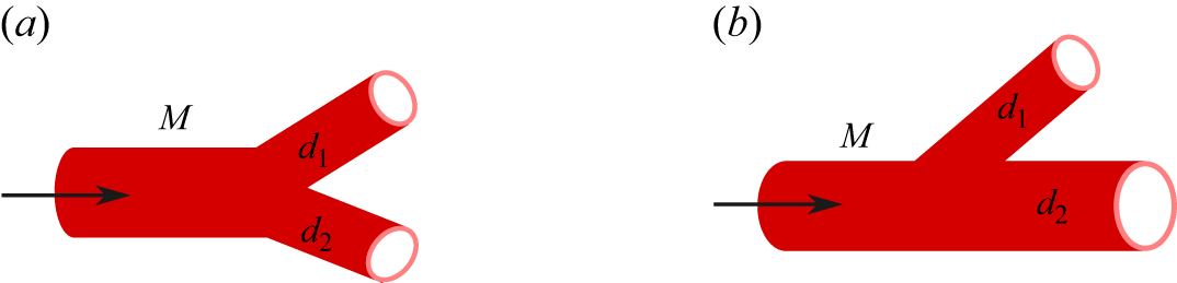


 fmean
 r/Rt
 (rn,θn)=(0.19Rt,2π/3)
 θ

 Rm,n
 m
 rn=0.19Rt
 αexch=2×10⁻⁵μmsg−1
 αexch=2×10⁻⁴μmsg−1
 αexch=2×10⁻³μmsg−1
 αexch=2×10⁻²μmsg−1
 kcap=0.03μm2
 kt=2×10⁻⁴μm2

 Em,m+1
 m
 rn=0.19Rt
 αexch=2×10⁻⁵μmsg−1
 αexch=2×10⁻⁴μmsg−1
 αexch=2×10⁻³μmsg−1
 αexch=2×10⁻²μmsg−1
 kcap=0.03μm2
 kt=2×10⁻⁴μm2

 fexch
 r/Rt
 rn=0.19Rt
 θn=2π/3
 M=26
 θ
 αexch=2×10⁻⁵μmsg−1
 αexch=2×10⁻⁴μmsg−1
 αexch=2×10⁻³μmsg−1
 kcap=0.03μm2
 kt=2×10⁻⁴μm2


 M