2 Problem formulation

We consider the system of partial differential equations representing the one-dimensional, inviscid, self-gravitating interstellar gas cloud with spherical symmetry. We assume the value of $\gamma $ , the adiabatic index, to be $5/3$ for the interstellar gas where $\displaystyle \gamma =c_{p}/c_{v}$ , where $c_{p}$ is the specific heat of the gas at constant pressure, and $c_{v}$ is the specific heat of the gas at constant volume. We consider the following system of governing equations, the details of the theories and derivations of which can be found in the literature [Reference Disney, McNally and Wright8–Reference Ferraioli and Virgopia10]:

(2.1) $$ \begin{align} & \rho_{t}+u\rho_{r}+\rho u_{r}+\frac{2\rho u}{r}=0,\nonumber\\ & u_{t}+uu_{r}+\frac{1}{\rho} p_{r}=g, \nonumber\\ &p_{t}+up_{r}+\rho a^{2}\bigg(u_{r}+\frac{2u}{r}\bigg)=-\frac{2}{3}\rho L(p,\rho),\nonumber\\ & g_{t}+ug_{r}+\frac{2gu}{r}=0, \end{align} $$

with equation of state $p=\rho RT,$ where t is time, u is the velocity of the particle along r, $\rho $ the density, g the acceleration due to gravity, p is the pressure, $L(p,\rho )$ is the cooling–heating function, $\displaystyle a=(\gamma p/\rho )^{1/2}$ is the isentropic speed of sound in gas, R the gas constant, and T the temperature. Unless otherwise stated, a variable as a subscript will indicate partial derivative with respect to that variable.

System of equations (2.1) can also be written in matrix form as

$$ \begin{align*} U_{t}+AU_{r}=f, \end{align*} $$

where

$$ \begin{align*}U=({\kern1pt}\rho, u, p, g)^{tr}, \quad f=\bigg(\displaystyle \frac{-2\rho u}{r}, g, -\bigg(\frac{2}{3}\rho L(p,\rho)+\frac{5}{3}\frac{2pu}{r}\bigg), -\frac{2gu}{r}\bigg)^{tr},\end{align*} $$

(2.2) $$ \begin{align} A=\left( \begin{array}{cccc} u & \rho & 0 & 0 \\ 0 & u & 1/\rho & 0 \\ 0 & \rho a^{2} & u & 0 \\ 0 & 0 & 0 & u \\ \end{array} \right), \end{align} $$

in which $tr$ denotes transposition.

The shock front $r=R(t)$ propagates into the nonhomogeneous medium with velocity $\displaystyle V=dR/dt$ and the following boundary conditions:

$$ \begin{align*} \rho_{0}=\rho_{0}(x),\hspace{1em} u_{0}=0,\hspace{1em} p_{0}=\mbox{constant},\hspace{1em} g_{0}=g_{0}(x). \end{align*} $$

System (2.1) in the conservation form behind and ahead of the shock is represented as

(2.3) $$ \begin{align} &G_{t}(r,t,U)+F_{r}(r,t,U)=H(r,t,U),\nonumber\\ &G_{*t}(r,t,U_{*})+F_{*r}(r,t,U_{*})=H_{*}(r,t,U_{*}). \end{align} $$

Here, U and $U_{*}$ characterize the solution vectors behind and ahead of the shock respectively, and

(2.4) $$ \begin{align} &G(r,t,U)=\big({\kern1pt}\rho, \rho u, \tfrac{1}{2}(3p+\rho u^{2}), \rho g\big)^{tr},\nonumber\\ &F(r,t,U)=\big({\kern1pt}\rho u, \rho u^{2}+p, \tfrac{1}{2}(5p+\rho u^{2})u, \rho ug\big)^{tr},\nonumber\\ &H(r,t,U)=\bigg(\frac{-2\rho u}{r}, \rho g-\bigg(\frac{2\rho u^{2}}{r}\bigg), \rho(ug-L)-\frac{u}{r}(5p+\rho u^{2}), -\frac{4\rho gu}{r}\bigg)^{tr}. \end{align} $$

Further, on using the Rankine–Hugoniot conditions $|[G]|V=|[F]|$ , where V is the shock velocity and the symbol $|[N]|=N-N_{0}$ is the jump in the variable N across the wave front entailing $N_{0}$ and N as the value just ahead and just behind the shock [Reference Jena15], we obtain

(2.5) $$ \begin{align} &\rho(R(t),t)=\frac{4\rho_{0}^{2}(R(t))V^{2}}{\rho_{0}(R(t))V^{2}+5p_{0}}, \hspace{1em} u(R(t),t)=\frac{3\rho_{0}(R(t))V^{2}-5p_{0}}{4\rho_{0}(R(t))V},\nonumber\\ &p(R(t),t)=\frac{3\rho_{0}(R(t))V^{2}-p_{0}}{4}, \hspace{1em} g(R(t),t)=g_{0}(R(t)). \end{align} $$

3 Similarity analysis by invariance group

We assume the existence of self-similar solutions of differential equations (2.1) and hence use the following one-parameter Lie group of transformations:

(3.1) $$ \begin{align} &x^{*}_{j}=x_{j}+\epsilon \zeta^{j}_{x}(x_{1},x_{2},u_{1},u_{2},u_{3},u_{4}), \quad j=1,2,\nonumber\\ &u^{*}_{i}=u_{i}+\epsilon \zeta^{i}_{u}(x_{1},x_{2},u_{1},u_{2},u_{3},u_{4}),\quad i=1,2,3,4, \end{align} $$

where $x_{1}=t$ , $x_{2}=r$ , $u_{1}=\rho $ , $u_{2}=u$ , $u_{3}=p$ , $u_{4}=g$ , $\epsilon $ is the parameter of the Lie group of transformations and $\zeta ^{j}_{x}$ and $\zeta ^{i}_{u}$ are the infinitesimals of the Lie group of transformations. Here, we use $p^{i}_{j}=\partial u_{i}/\partial x_{j}$ , and rewrite the system of equations (2.1) in the form

$$ \begin{align*} F_{k}(x_{j},u_{i},p^{i}_{j})=0, \quad k=1,2,3,4, \end{align*} $$

which are constantly, conformally invariant [Reference Hansen11] under the infinitesimal group (3.1), if there exist constants $\alpha _{rs} (r,s=1,2,3,4)$ such that for all smooth surfaces, $u_{i}=u_{i}(x_{j})$ , we have

$$ \begin{align*} SF_{k}=\alpha_{kr}F_{r},\quad k=1,2,3,4, \end{align*} $$

where S denotes the Lie derivative in the direction of the extended field vector and is given as

$$ \begin{align*} S=\zeta^{j}_{x}\frac{\partial}{\partial x_{j}}+\zeta^{i}_{u}\frac{\partial}{\partial u_{i}}+\zeta^{i}_{p_{j}}\frac{\partial}{\partial p^{i}_{j}}, \end{align*} $$

with

$$ \begin{align*} \zeta^{i}_{p_{j}}=\frac{\partial \zeta^{i}_{u}}{\partial x_{j}}+\frac{\partial \zeta^{i}_{u}}{\partial u_{k}}p^{k}_{j}-\frac{\partial \zeta^{l}_{x}}{\partial x_{j}}p^{i}_{l}-\frac{\partial \zeta^{l}_{x}}{\partial u_{n}}p^{i}_{l}p^{n}_{j} \end{align*} $$

being the infinitesimals of derivative of the transformation. We obtain the following forms of infinitesimals $\zeta ^{j}_{x}$ and $\zeta ^{i}_{u}$ from (2.1) by using the above procedure:

(3.2) $$ \begin{align} &\zeta^{1}_{x}=ax_{1}+b, &&\zeta^{2}_{x}=(\alpha_{22}-\alpha_{11}+a)x_{2},\nonumber\\ &\zeta^{1}_{u}=(\alpha_{11}+a)u_{1}, &&\zeta^{2}_{u}=(\alpha_{22}-\alpha_{11})u_{2},\nonumber\\ &\zeta^{3}_{u}=(2\alpha_{22}-\alpha_{11}+a)u_{3}, &&\zeta^{4}_{u}=(\alpha_{22}-\alpha_{11}-a)u_{4},\nonumber\\ &L=u_{1}^{(2(\alpha_{22}-\alpha_{11})-a)/(\alpha_{11}+a)}L^{*}(\phi), &&\phi=u_{3}u_{1}^{-(2\alpha_{22}-\alpha_{11}+a)/(\alpha_{11}+a)}, \end{align} $$

where a, b, $\alpha _{11}$ , $\alpha _{22}$ are arbitrary constants, and $L^{*}$ is an arbitrary function of its arguments. We consider the following cases based on the presence of arbitrary constants.

3.1 Case I

When $a \neq 0$ and $\alpha _{22}-\alpha _{11}+a \neq 0$ , the translational invariance of $x_{1}$ given by $\tilde {x_{1}}=x_{1}+b/a$ on suppressing the tilde, yields from the first equation in (3.2) that $\zeta ^{1}_{x}=ax_{1}$ , while the other equations in (3.2) remain unchanged. Using the invariant surface conditions, $u_{i}(x^{*},t^{*})=u^{*}_{i}(x,t)$ , we have

(3.3) $$ \begin{align} \frac{dx_{1}}{\zeta^{1}_{x}}=\frac{dx_{2}}{\zeta^{2}_{x}}=\frac{du_{1}}{\zeta^{1}_{u}}=\frac{du_{2}}{\zeta^{2}_{u}}=\frac{du_{3}}{\zeta^{3}_{u}}=\frac{du_{4}}{\zeta^{4}_{u}}. \end{align} $$

The parameters are nondimensionalized using

$$ \begin{align*} &\tilde{r}=\frac{r}{r_{c}}, \quad \tilde{t}=\frac{t}{t_{c}}, \quad \tilde{u}=\frac{ut_{c}}{r_{c}}, \quad \tilde{\rho}=\frac{\rho}{\rho_{c}},\nonumber\\ & \tilde{p}=\frac{pt_{c}^{2}}{\rho_{c}r_{c}^{2}}, \quad \tilde{g}=\frac{gt_{c}^{2}}{r_{c}}, \quad \tilde{a}=\frac{at_{c}}{r_{c}}, \quad \tilde{L}(\tilde{p},\tilde{\rho})=\frac{t_{c}^{3}}{r_{c}^{2}}L(p,\rho),\nonumber \end{align*} $$

where $r_{c}$ , $t_{c}$ and $\rho _{c}$ are reference values of r, t and $\rho $ , respectively.

Further, using equations (3.2) along with the nondimensional form of the variables in equation (3.3), the following forms of flow variables $\rho $ , u, p, g and the cooling–heating function L are obtained:

(3.4) $$ \begin{align} \rho=t^{\mu}S(\xi),\hspace{1em} u=t^{(\delta-1)}U(\xi),\hspace{1em} p=t^{(2(\delta -1)+\mu)}P(\xi),\nonumber\\ g=t^{(\delta-2)}G(\xi),\hspace{1em} L(p,\rho)=\rho^{(2\delta-3)/\mu}L^{*}(\phi),\qquad \ \ \, \end{align} $$

where $\xi =rt^{-\delta },$ is the dimensionless similarity variable

$$ \begin{align*}\mu=(\alpha_{11}+a)/a,\quad \delta=(\alpha_{22}-\alpha_{11}+a)/a,\quad \phi=PS^{-(2(\delta-1)+\mu)/\mu}, \end{align*} $$

and S, U, P, G and $L^{*}$ are arbitrary functions of their arguments.

Since the shock must be a similarity curve, it may be normalized to be at $\xi =1$ which then yields the shock path $R(t)$ , the shock velocity $V(t)$ and the flow variables in the form

(3.5) $$ \begin{align} &R(t)=t^{\delta},\hspace{1em} V(t)=\delta t^{(\delta-1)}, && \rho|_{\xi=1}=t^{\mu}S(1), \hspace{1em} u|_{\xi=1}=t^{(\delta-1)}U(1),\nonumber\\ &p|_{\xi=1}=t^{(2(\delta-1)+\mu)}P(1),&& e g|_{\xi=1}=t^{(\delta-2)}G(1). \end{align} $$

From equation (3.5) and (2.5) we obtain

(3.6) $$ \begin{align} &S(1)=\frac{4\rho_{0}^{2}(R(t))V^{2}}{\rho_{0}(R(t))V^{2}+5p_{0}}t^{-\mu}, && U(1)=\frac{3\rho_{0}(R(t))V^{2}-5p_{0}}{4\rho_{0}(R(t))V^{2}}t^{(1-\delta)},\nonumber\\ &P(1)=\frac{3\rho_{0}(R(t))V^{2}-p_{0}}{4\rho_{0}(R(t))V^{2}}t^{-(2(\delta-1)+\mu)}, && G(1)=g_{0}(R(t))t^{-(\delta-2)}. \end{align} $$

In the case of a shock of arbitrary strength, the above relations from equation (3.6) imply that $\rho _{0}V^{2}$ must be a constant and further provide that $\rho _{0}$ and $g_{0}$ must satisfy the power law in r such that $\rho _{0}=r^{\theta }$ and $g_{0}=r^{\kappa }$ . Also, the jump conditions (3.6) signify that $\kappa =(\delta -2)/\delta $ along with the condition that for a shock of arbitrary strength ${\delta \theta +2(\delta -1)=0}$ and for a strong shock $\delta \theta =\mu $ . Hence, from equation (3.4) we get

(3.7) $$ \begin{align} &\rho=\rho_{0}(R(t))S^{*}(\xi),\hspace{1em} u=VU^{*}(\xi),\nonumber\\ &p=\rho_{0}(R(t))V^{2}P^{*}(\xi),\hspace{1em} g=g_{0}(R(t))G^{*}(\xi), \end{align} $$

where $S^{*}(\xi )=S(\xi )$ , $U^{*}(\xi )=U(\xi )/\delta $ , $P^{*}(\xi )=P(\xi )/\delta ^{2}$ and $G^{*}(\xi )=G(\xi )$ .

Using equations (3.4), (3.7) and (2.1), a system of ordinary differential equations in $S^{*}$ , $U^{*}$ , $P^{*}$ and $G^{*}$ is obtained, which on suppressing the asterisk becomes

(3.8) $$ \begin{align} &(U-\xi)S'+\theta S+SU'+\frac{2US}{\xi}=0,\nonumber\\ &(U-\xi)U'+\frac{\delta-1}{\delta}U+\frac{P'}{S}=\frac{G(\xi)}{\delta^{2}},\nonumber\\ &(U-\xi)P'+\bigg(\frac{2(\delta-1)}{\delta}+\theta +\frac{5}{3}\bigg(U'+\frac{2U}{\xi}\bigg)\bigg)P=-\frac{2}{3\delta}(S(\xi))^{(2\delta -3+\mu)/\mu}L^{*}(\phi),\nonumber\\ &(U-\xi)G'+\frac{(\delta-2)}{\delta}G=-\frac{2UG}{\xi}. \end{align} $$

Here, a primes denote differentiation with respect to the independent variable $\xi $ and $\phi =\delta ^{2}PS^{-(2(\delta -1)+\mu )/\mu }$ . The above system of equations (3.8) satisfy the following jump conditions for a shock of arbitrary strength:

(3.9) $$ \begin{align} &S(1)=\frac{4\rho_{0}^{2}(R(t))V^{2}}{\rho_{0}(R(t))V^{2}+5p_{0}}, \hspace{1em} U(1)=\frac{3\rho_{0}(R(t))V^{2}-5p_{0}}{4\rho_{0}(R(t))V^{2}},\nonumber\\ &P(1)=\frac{3\rho_{0}(R(t))V^{2}-p_{0}}{4\rho_{0}(R(t))V^{2}}, \hspace{1em} G(1)=1, \end{align} $$

and for an infinitely strong shock

(3.10) $$ \begin{align} S(1)=4,\hspace{1em} U(1)=\tfrac{3}{4}, \hspace{1em} P(1)=\tfrac{3}{4}, \hspace{1em} G(1)=1. \end{align} $$

3.2 Particular solution

Self-similar solutions are of two types. In the solutions of the first type, the similarity exponent $\delta $ is determined either by dimensional considerations or from conservation laws. In the second type of solutions, the determination of the similarity exponent requires that the ordinary differential equations for the reduced functions be integrated, since $\delta $ cannot be found from dimensional considerations or from the conservation laws without solving the equations as in first type. In this paper we have considered the case of self-similarity of the second type. Since the system of equations (3.8) cannot be solved analytically to obtain an exact solution, any particular solution of the system is of practical importance to get an idea of the nature of the solutions. Equations (3.8) with shock conditions (3.10) admit particular solutions for U, S, P and G as

(3.11) $$ \begin{align} U=\tfrac{3}{4}\xi, \hspace{1em} S=4\xi^{4\theta +9},\hspace{1em} P=\tfrac{3}{4}\xi^{4\theta +11},\hspace{1em} G=\xi, \end{align} $$

where the similarity exponent $\displaystyle \delta =8/9$ and $\displaystyle \theta =-11/16$ . The form of the cooling–heating function L is

$$ \begin{align*} L(p,\rho)=\rho^{2}L^{*}(\phi),\hspace{1em} L^{*}(\phi)=\phi^{m}, \end{align*} $$

with

(3.12) $$ \begin{align} \phi=\frac{4^{7/11}\xi^{-3/11}}{27}, \hspace{1em} m=\frac{77}{2}. \end{align} $$

Using relations (3.11)–(3.12), the flow variables are given by

(3.13) $$ \begin{align} \rho&=\rho_{0}(R(t))S(\xi), &u&=VU(\xi),\nonumber\\ p&=\rho_{0}V^{2}P(\xi), &g&=g_{0}(R(t))G(\xi), \end{align} $$

where

$$ \begin{align*} &R(t)=t^{8/9},&& V=\tfrac{8}{9}t^{-1/9},&& \rho_{0}(R(t))=t^{(8/9)\theta},\nonumber\\ &p_{0}(R(t))=\mbox{constant},&& g_{0}(R(t))=t^{-80/81},&& u_{0}(R(t))=0. \end{align*} $$

3.3 Case II

When $(\alpha _{22}-\alpha _{11}) \neq 0$ and $a=0$ , from equations (3.6) and (3.8) we get the following form of flow variables and cooling–heating function:

(3.14) $$ \begin{align} &\rho=\rho_{0}(R(t))S^{*}(\xi),&& u=VU^{*}(\xi),&& p=\rho_{0}(R(t))V^{2}P^{*}(\xi),\nonumber\\ &g=g_{0}(R(t))G^{*}(\xi),&& L(p,\rho)=\rho^{2\delta/\mu}L^{*}(\phi),&& \phi=P^{*}S^{*-(2\delta +\mu)/\mu}, \end{align} $$

where the dimensionless similarity variable $\xi $ , the shock location R at $\xi =1$ , the shock velocity V, $\rho _{0}(x)$ and $g_{0}(x)$ are given by

(3.15) $$ \begin{align} \xi=re^{-\delta t},\hspace{1em} R=e^{\delta t},\hspace{1em} V=\delta e^{\delta t},\hspace{1em} \rho_{0}(x)=x^{\theta},\hspace{1em} g_{0}=r, \end{align} $$

with $\delta =(\alpha _{22}-\alpha _{11})/b$ , $\mu =\alpha _{11}/b=\theta \delta $ . Note that this case leads to a class of similarity solutions with an exponential shock path given by (3.14).

Now using equations (3.14) and (3.15) in (2.1) and suppressing the asterisk, we obtain the following set of ordinary differential equations:

(3.16) $$ \begin{align} &(U-\xi)S'+\theta S+SU'+\frac{2US}{\xi}=0,\nonumber\\ &(U-\xi)U'+U+\frac{P'}{S}=\frac{G(\xi)}{\delta^{2}},\nonumber\\ &(U-\xi)P'+\bigg\{2+\theta +\frac{5}{3}\bigg(U'+\frac{2U}{\xi}\bigg)\bigg\}P=-\frac{2}{3\delta}(S(\xi))^{(2\delta +\mu)/\mu}L^{*}(\phi),\nonumber\\ &(U-\xi)G'+G=-\frac{2UG}{\xi}. \end{align} $$

In this case, $\phi =\delta ^{2}PS^{-(2\delta +\mu )/\mu }$ . The system of equations (3.16) can be solved using the jump conditions (3.9) or (3.10), depending on a shock of arbitrary strength or an infinitely strong shock, respectively.

4 Acceleration wave front

We take the flow variables $\rho $ , u, p, g to be continuous, but we may encounter discontinuities in their first-order derivatives across the associated propagating wave surface. The equation of the wave front $\Phi $ is expressed as $r=\chi (t)$ , providing the flow parameters as functions of t only. The kinematic and geometric compatibility conditions of first and second order for a singular surface [Reference Thomas32] are given by

$$ \begin{align*} |[J_{x}]|=B,\hspace{1em} |[J_{t}]|=-ZB,\hspace{1em} |[J_{xx}]|=\overline{B},\hspace{1em} |[J_{xt}]|=Z(B_{x}-\overline{B}), \end{align*} $$

where J represents any of the flow variables, and $Z=d\chi /dt$ denotes the speed at which $\Phi $ propagates.

The matrix A in equation (2.2) has eigenvalues $\lambda ^{(1)}=u+a$ , $\lambda ^{(2)}=u$ (a double root) and $\lambda ^{(3)}=u-a$ . The corresponding eigenvectors are:

$$ \begin{align*} &L^{(1)}=(0,\rho a,1,0), && R^{(1)}=(1/(2a^{2}),1/(2\rho a),1/2,0)^{tr},\nonumber\\ &L^{(2,1)}=(-a^{2},0,1,0),&& R^{(2,1)}=(-a^{-2},0,0,-1/(ga^{2}))^{tr},\nonumber\\ &L^{(2,2)}=(0,0,0,1), && R^{(2,2)}=(u^{-2},0,0,a^{-2})^{tr},\nonumber \\ &L^{(3)}=(0,-\rho a,1,0), && R^{(3)}=(1/(2a^{2}),-1/(2\rho a),1/2,0)^{tr}.\nonumber \end{align*} $$

As per the assumption of spherical symmetry of cloud model, the wave travels towards the centre for which there arise two cases due to the presence of the unperturbed state, that is, on the left-hand side or the right-hand side of the moving wave front. If the unperturbed state is considered to be on the right-hand side or on the left-hand side, then $Z=u+a$ or $Z=u-a$ , respectively. Using the following relations in the system of equations (2.1) on the inner boundary of $\Phi $ ,

(4.1) $$ \begin{align} &|[{\kern1pt}\rho_{r}]|=\varrho,&& |[u_{r}]|=\alpha^{(1)},&& |[p_{r}]|=\xi,&& |[g_{r}]|=\eta, \nonumber\\ & |[{\kern1pt}\rho_{t}]|=-Z\varrho,&&|[u_{t}]|=-Z\alpha^{(1)}, &&|[p_{t}]|=-Z\xi,&& |[g_{t}]|=-Z\eta, \end{align} $$

and simplifying, we obtain

$$ \begin{align*} Z=u_{0}\pm a_{0}, \hspace{1em} \alpha^{(1)}=\pm \frac{1}{\rho_{0}a_{0}}\xi=\pm \frac{a_{0}}{\rho_{0}}\varrho \hspace{1em} \mbox{and} \hspace{0.5em} \eta=0. \end{align*} $$

Now we have the following set of compatibility conditions:

(4.2) $$ \begin{align} &|[{\kern1pt}\rho_{rr}]|=\overline{\varrho},&& |[u_{rr}]|=\overline{\alpha^{(1)}},&&|[p_{rr}]|=\overline{\xi}, &&|[g_{rr}]|=\overline{\eta}, \nonumber\\ & |[{\kern1pt}\rho_{rt}]|=Z(\varrho_{r}-\overline{\varrho}),&&|[u_{rt}]|=Z(\alpha^{(1)}_{r}-\overline{\alpha^{(1)}}),&& |[p_{rt}]|=Z(\xi_{r}-\overline{\xi}),&& |[g_{rt}]|=Z(\eta_{r}-\overline{\eta}). \end{align} $$

Differentiating system (2.1) with respect to r and evaluating behind the wave front $\Phi $ , we get

(4.3) $$ \begin{align} &|[{\kern1pt}\rho_{rt}]|+2|[u_{r}\rho_{r}]|+u_{0}|[{\kern1pt}\rho_{rr}]|+\rho_{0}|[u_{rr}]|+\frac{2u_{0}}{r}|[{\kern1pt}\rho_{r}]|+\frac{2\rho_{0}}{r}|[u_{r}]|=0,\nonumber\\ &|[u_{rt}]|+u_{0}|[u_{rr}]|+|[u_{r}u_{r}]|+\frac{1}{\rho_{0}}|[p_{rr}]|-\frac{1}{\rho_{0}^{2}}|[p_{r}\rho_{r}]|-|[g_{r}]|=0,\nonumber\\ &|[p_{rt}]|+\frac{8}{3}|[u_{r}p_{r}]|+u_{0}|[p_{rr}]|+\frac{5}{3}p_{0}\bigg(|[u_{rr}]|+\frac{2}{r}|[u_{r}]|\bigg)+\frac{10}{3}\frac{u_{0}|[p_{r}]|}{r}\nonumber\\ &\quad\quad =-\frac{2}{3}\{L_{0}|[{\kern1pt}\rho_{r}]|+\rho_{0}((L_{\rho})_{0}|[{\kern1pt}\rho_{r}]|+(L_{p})_{0}|[p_{r}]|)\},\nonumber\\ &|[g_{rt}]|+|[u_{r}g{r}]|+u_{0}|[g_{rr}]|+\frac{2}{r}u_{0}|[g_{r}]|+\frac{2}{r}g_{0}|[u_{r}]|=0. \end{align} $$

Using equations (4.1) and (4.2) in (4.3), we obtain

(4.4) $$ \begin{align} &Z(\varrho_{r}-\overline{\varrho})+2((\varrho+\rho_{0r})\alpha^{(1)}+\varrho u_{0r})+u_{0}\overline{\varrho}+\rho_{0}\overline{\alpha^{(1)}}+\frac{2}{r}(u_{0}\varrho+\rho_{0}\alpha^{(1)})=0,\nonumber\\ &Z(\alpha^{(1)}_{r}-\overline{\alpha^{(1)}})+u_{0}\overline{\alpha^{(1)}}+(\alpha^{(1)})^{2}+\frac{1}{\rho_{0}}\overline{\xi}-\frac{1}{\rho_{0}^{2}}(\varrho(\xi+p_{0x})+\rho_{0r}\xi)+2\alpha^{(1)} u_{0r}=0,\nonumber\\ &Z(\xi_{r}-\overline{\xi})+\frac{8}{3}(\alpha^{(1)}(\xi+p_{0r})+u_{0r}\xi)+u_{0}\overline{\xi}+\frac{5}{3}p_{0}\bigg(\overline{\alpha^{(1)}}+\frac{2\alpha^{(1)}}{r}\bigg)+\frac{10}{3}\frac{u_{0}\xi}{r} \nonumber\\ &\quad =-\frac{2}{3}(\varrho L_{0}+\rho_{0}((L_{\rho})_{0} \varrho+(L_{p})_{0}\xi)),\nonumber\\ &\alpha^{(1)}g_{0r}-a_{0}\overline{\eta}+\frac{2}{r}g_{0}\alpha^{(1)}=0. \end{align} $$

Considering the unperturbed state to be on the right-hand side and eliminating $\overline {\varrho }$ , $\overline {\alpha ^{(1)}}$ and $\overline {\xi }$ from equation (4.4) and further using equation (3.13), we obtain the following Bernoulli type of transport equation [Reference Jeffrey13] for $\alpha ^{(1)}$ :

(4.5) $$ \begin{align} 2\frac{d\alpha^{(1)}}{dt}+\frac{8}{3}(\alpha^{(1)})^{2}\pm \Theta\alpha^{(1)}=0, \end{align} $$

where

$$ \begin{align*} \Theta=\frac{14u_{0r}}{3}-\frac{\rho_{0r}a_{0}}{\rho_{0}}+\frac{5p_{0r}}{3\rho_{0}a_{0}}+\frac{10u_{0}}{3r}+\frac{2a_{0}}{r}+ \frac{2}{3}\bigg(\frac{L_{0}}{a_{0}^{2}}+\frac{(L_{\rho})_{0}\rho_{0}}{a_{0}^{2}}+(L_{p})_{0}\rho_{0}\bigg). \end{align*} $$

Integration of equation (4.5) yields the solution

(4.6) $$ \begin{align} \alpha^{(1)}(t)=\alpha^{(1)}_{0}\eta(t)\bigg\{1+\frac{4\alpha^{(1)}_{0}}{3}\int_{t_{0}}^{t}\eta(w)\,dw\bigg\}^{-1}, \end{align} $$

with $ \eta (t)=\exp (-\tfrac 12\int _{t_{0}}^{t}\Theta (w)\,dw)$ .

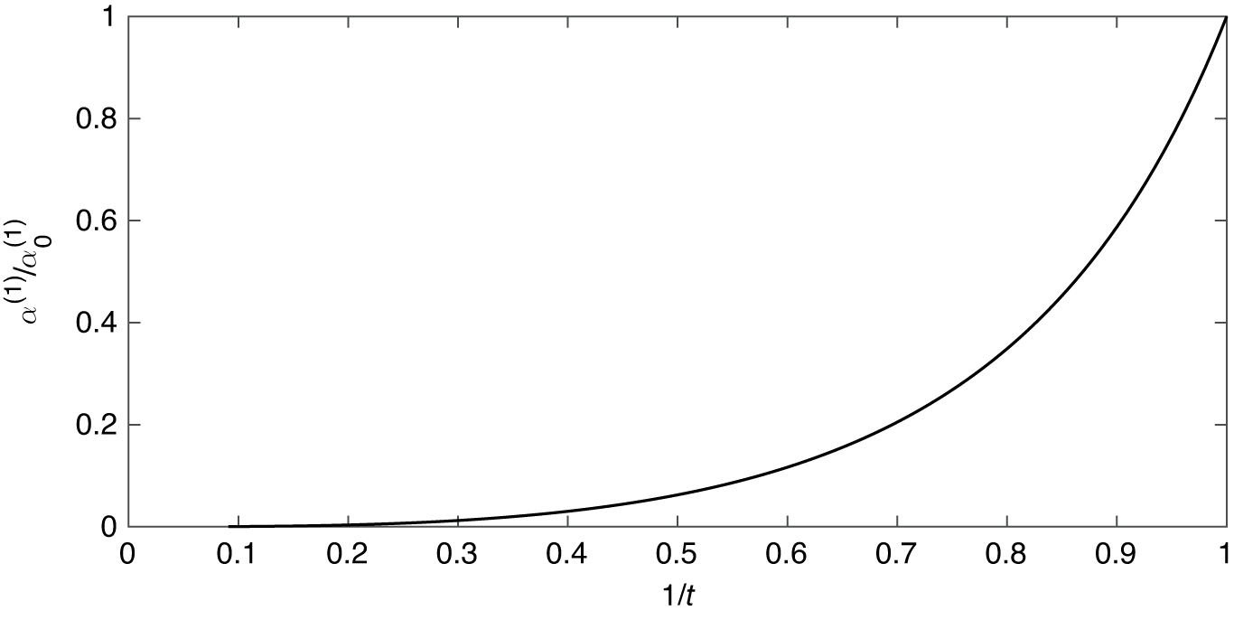
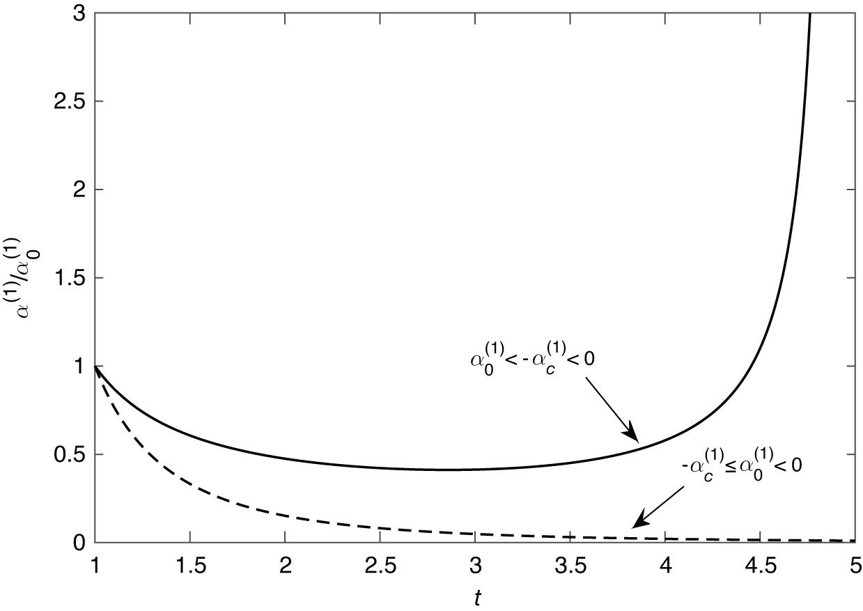
The results are depicted in Figure 1 for rarefaction waves ( $\alpha ^{(1)}_{0}>0$ ) and in Figure 2 for compression waves ( $\alpha ^{(1)}_{0}<0$ ). From Figure 1, it is observed that the amplitude of the jump in velocity gradient $\alpha ^{(1)}$ decreases as time increases and dies out eventually. In contrast, from Figure 2 it is observed that the solution breaks down when the denominator in equation (4.6) (that is, $ 1+(4\alpha ^{(1)}_{0}/3)\int _{t_{0}}^{t}\eta (w)\,dw$ ) equals zero at some time $t=t_{c}$ , implying the existence of a steepened wave in a finite time only. Further, the following cases arise from equation (4.6).

Figure 1

Jump in velocity gradient $\alpha ^{(1)}$ varying with $1/t$ for rarefaction waves ( $\alpha ^{(1)}_{0}>0$ ).

Figure 2

Jump in velocity gradient $\alpha ^{(1)}$ varying with $1/t$ for compression waves ( $\alpha ^{(1)}_{0}<0$ ).

1. (1) The conditions $\displaystyle |\alpha ^{(1)}_{0}|/\alpha ^{(1)}_{c} < 1$ and $\displaystyle |\alpha ^{(1)}_{0}|/\alpha ^{(1)}_{c} = 1$ , where $\displaystyle \alpha ^{(1)}_{c}=1/I\{\infty \}$ with $I(t)=(4/3)\int _{t_{0}}^{t}\eta (w)\,dw$ lead to $\displaystyle \alpha ^{(1)} \rightarrow 0$ , showing the existence of a flattened wave as time advances.

2. (2) For $\displaystyle |\alpha ^{(1)}_{0}|/\alpha ^{(1)}_{c}> 1$ , there exists a finite time $t_{c}$ such that $\displaystyle I(t_{c})=1/|\alpha ^{(1)}_{0}|$ and $|\alpha ^{(1)}| \rightarrow \infty $ as $t \rightarrow t_{c}$ . This yields the existence of a shock wave in a finite time only at an instant $t_{c}$ .

The results depicted are for the case where the unperturbed state is on the right-hand side. Similar results have been obtained for the case where the unperturbed state is on the left-hand side, and hence omitted.

5 Amplitudes of reflected and transmitted waves

The concepts of reflected and transmitted waves come into existence by the phenomena of interaction between nonlinear waves. The amplitudes of these reflected and transmitted waves are imperative to study and establish the results of collision. In this paper, the conservation form of the system in equation (2.3) behind and ahead of the shock front makes it viable to study the amplitudes. We consider the interaction of the strong shock and the fastest moving discontinuity which originates from the point $(r_{0},t_{0})$ , and propagates along the characteristic $dx/dt=\lambda ^{(1)},$ represented as $\phi (x,t)=0$ . Let $M(x_{m},t_{m})$ be the point of intersection of the moving wave with the shock path.

For a strong shock, $p_{0}\ll V$ , and hence the Rankine–Hugoniot jump conditions in equation (2.5) yield

(5.1) $$ \begin{align} &\rho(R(t),t)=4\rho_{0}, \quad u(R(t),t)=\frac{3V}{4}, \quad p(R(t),t)=\frac{3\rho_{0}V^{2}}{4},\nonumber\\ &g(R(t),t)=g_{0}(R(t)). \end{align} $$

Further, in the case of strong shock, we obtain the speed of sound as $a= \sqrt {5}V/4$ and the eigenvalues as

(5.2) $$ \begin{align} &\lambda^{(1)}=\frac{3V}{4}+\frac{\sqrt{5}V}{4},&& \lambda_{*}^{(1)}=\bigg(\frac{5p_{0}}{3\rho_{0}}\bigg)^{1/2},\nonumber\\ &\lambda^{(2)}=\frac{3V}{4},&& \lambda_{*}^{(2)}=0,\nonumber \\ &\lambda^{(3)}=\frac{3V}{4}-\frac{\sqrt{5}V}{4}, && \lambda_{*}^{(3)}=-\bigg(\frac{5p_{0}}{3\rho_{0}}\bigg)^{1/2}. \end{align} $$

The evolutionary conditions of the reflected and transmitted waves given by Lax [Reference Lax19] are formulated as

$$ \begin{align*} && \lambda^{(p)}<\lambda^{(p-1)}<\cdots<\lambda^{(l+1)}<V<\lambda^{(l)}<\cdots<\lambda^{(1)},\nonumber\\ &&\lambda^{(p)}_*<\lambda^{(p-1)}_*<\cdots<\lambda^{(l)}_*<V<\lambda^{(l-1)}_*<\cdots<\lambda^{(1)}_*. \end{align*} $$

In the present problem, we have the inequalities

$$ \begin{align*} \lambda^{(3)}<\lambda^{(2)}<V<\lambda^{(1)} \hspace{1em}\mbox{and}\hspace{1em} \lambda^{(3)}_*<\lambda^{(2)}_*<\lambda^{(1)}_*<V, \end{align*} $$

which imply that in this case of collision between a weak discontinuity travelling with velocity $\lambda ^{(1)}$ at time $t=t_{m}$ and strong shock, there are two reflected waves moving with velocity $\lambda ^{(2)}$ and $\lambda ^{(3)}$ and no transmitted waves. The new wavefront from point M after interaction propagates through the characteristic $dr/dt=\lambda _{*}^{(1)}$ , and is represented as $\phi _{*}(r,t)=0$ . Then, following the above discussion, the jumps in $U_{r}$ across the incident and reflected waves at M are given by

$$ \begin{align*} \wedge_{1}(M)=\sum_{k=1}^{n_{1}}\alpha_{k}^{(1)}(t_{m})R_{s}^{(1,k)},\hspace{1em} \wedge_{i}^{(R)}(M)=\sum_{k=1}^{n_{i}}\alpha_{k}^{(i)}(t_{m})R_{s}^{(i,k)}, \end{align*} $$

with subscript s specifying the values calculated at the point M. The evolutionary equations deducing the amplitudes $\alpha _{k}^{(i)}$ of reflected waves along with the jump in the shock acceleration $|[\dot {V}]|$ at time $t=t_{m}$ in the absence of transmitted waves are obtained by the system of algebraic equations given as

$$ \begin{align*} |[\dot{V}]|(G-G_{*})_{s}&+(\nabla G)_{s}\sum_{i=p-q+1}^{p}\bigg\{\sum_{k=1}^{m_{i}}\alpha_{k}^{(i)}(V-\lambda^{(i)})^{2}R_{s}^{(i,k)})\bigg\}\\ &\quad=-(\nabla G)_{s}\sum_{k=1}^{m_{1}}\alpha_{k}^{(1)}(V-\lambda^{(1)})^{2}R_{s}^{(1,k)},\nonumber \end{align*} $$

which simplifies to the following form in our problem:

$$ \begin{align*} (G-G_*)_s|[\dot{V}]|&+(\nabla G)_s R^{(3)}_s(V-\lambda^{(3)}_s)^2 \alpha^{(3)}+(\nabla G)_s R^{(2,1)}_s(V-\lambda_{s}^{(2)})^2 \alpha_{2}^{(1)}\nonumber\\ &+(\nabla G)_s R^{(2,2)}_s(V-\lambda_{s}^{(2)})^2 \alpha_{2}^{(2)}=-(\nabla G)_s R^{(1)}_s(V-\lambda^{(1)}_s)^2 \alpha^{(1)}. \end{align*} $$

Using (2.3), (2.4), (5.1) and (5.2), we get the system of algebraic equations

(5.3) $$ \begin{align} 3\rho_{0}|[\dot{V}]|&+\tfrac{1}{10}(1+\sqrt{5})^{2}\alpha^{(3)}-\tfrac{1}{5}\alpha_{2}^{(1)}+\tfrac{1}{9}\alpha_{2}^{(2)}=-\tfrac{1}{10}(1-\sqrt{5})^{2}\alpha^{(1)},\nonumber\\[-0.2pt] 3\rho_{0}|[\dot{V}]|&+\frac{1}{16}\bigg(\frac{6}{5}-\frac{2}{\sqrt{5}}\bigg)(1+\sqrt{5})^{2}\alpha^{(3)}-\frac{3}{20}\alpha_{2}^{(1)}+\frac{1}{12}\alpha_{2}^{(2)}\nonumber \\[-2pt] &\quad=-\frac{1}{16}\bigg(\frac{6}{5}+\frac{2}{\sqrt{5}}\bigg )(1-\sqrt{5})^{2}\alpha^{(1)},\nonumber\\[-2pt] \frac{9\rho_{0}}{4}|[\dot{V}]|&+\frac{1}{16}\bigg(\frac{6}{5}-\frac{3}{2\sqrt{5}}\bigg)(1+\sqrt{5})^{2}\alpha^{(3)}-\frac{9}{80}\alpha_{2}^{(1)}+\frac{1}{32}\alpha_{2}^{(2)}\nonumber \\[-2pt] &\quad=-\frac{1}{16}\bigg(\frac{6}{5}+\frac{3}{2\sqrt{5}}\bigg)(1-\sqrt{5})^{2}\alpha^{(1)},\nonumber\\[-2pt] 3\rho_{0}g_{0}|[\dot{V}]|&+\frac{g_{0}}{10}(1+\sqrt{5})^{2}\alpha^{(3)}-\bigg(\frac{g_{0}}{5}+\frac{4\rho_{0}}{5g_{0}}\bigg)\alpha_{2}^{(1)}+\bigg(\frac{g_{0}}{9}+\frac{4\rho_{0}}{5}\bigg)\alpha_{2}^{(2)}\nonumber\\[-2pt] &\quad=-\frac{g_{0}}{10}(1-\sqrt{5})^{2}\alpha^{(1)}. \end{align} $$

Solving this system of equations yields the amplitudes of the reflected waves and the jump in the shock acceleration in the following form:

$$ \begin{align*} \alpha_{2}^{(1)}&=\frac{-3g_{0}(1-\sqrt{5})^{2}}{20\sqrt{5}A}\alpha^{(1)},\nonumber\\ \alpha_{2}^{(2)}&=\frac{-3(1-\sqrt{5})^{2}}{20\sqrt{5} A}\alpha^{(1)},\nonumber\\ \alpha^{(3)}&=\frac{(1-\sqrt{5})^{2}\bigg(\displaystyle \frac{-3g_{0}}{100}-\frac{1}{8\sqrt{5}}+\frac{1}{24}\bigg)}{(1+\sqrt{5})^{2}A}\alpha^{(1)},\nonumber\\ |[\dot{V}]|&=\frac{(1-\sqrt{5})^{2}}{30\sqrt{5}\rho_{0}A}\bigg(\frac{-3g_{0}}{10}+\frac{5}{12}\bigg)\alpha^{(1)},\nonumber \end{align*} $$

where

$$ \begin{align*}A=\bigg(\displaystyle \frac{3g_{0}}{100}-\frac{1}{8\sqrt{5}}-\frac{1}{24}\bigg).\end{align*} $$

6 Results and conclusion

This paper considers the system of partial differential equations modelling the self-gravitating interstellar gas clouds in spherical symmetry. Using the Lie group of transformations, the governing system of partial differential equations reduces to a system of ordinary differential equations for obtaining self-similar solutions. Particular solutions are obtained for the flow variables and the cooling–heating function in the case of an infinitely strong shock. Further, singular surface theory is used to study the acceleration wave front, taking into account the particular solution so obtained. The Bernoulli type equation [Reference Jena15] for velocity gradient is obtained, which is solved numerically to analyse the variation of the velocity gradient with time. The numerical results are depicted, and we observe that the jump in velocity gradient decreases with increase in time and vanishes in the long run in the case of rarefaction waves. However, for compression waves, there exists a critical time at which the jump in velocity gradient becomes unbounded. The interaction between the strong shock and the singular surface is studied. We observe that there are no transmitted waves, and hence the amplitudes of reflected waves are obtained, which are directly proportional to the amplitude of the jump in velocity gradient.