
















1. Introduction
The present paper fits into the body of literature revolving around classifying maps between various matrix domains which preserve spectra or various other invariants/properties. A few recollections will help appreciate the general flavour of the topic.
Denote by  $M_n$ the algebra of
 $n\times n$ complex matrices, by
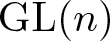
 $GL(n)$ its group of invertible elements, and by
 $U(n)$ the unitary group. It is well-known that any non-zero Jordan endomorphism
 $\phi$ of
 $M_n$ (i.e., [Reference Jacobson19, § I.1] a linear map
 $\phi:M_n\to M_n$ with
 $\phi(XY+YX) = \phi(X)\phi(Y) + \phi(Y)\phi(X)$ for all
 $X,Y \in M_n$) is either a conjugation by an invertible matrix, or a conjugation composed with transposition:
 \begin{equation}
\phi(\cdot) = T(\cdot)T^{-1} \qquad \text{or} \qquad \phi(\cdot) = T(\cdot)^{t}T^{-1},
\end{equation}
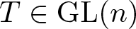
for some  $T \in GL(n)$ (see e.g., [Reference Herstein17, Reference Šemrl35]). There are numerous results in the ever-growing literature characterizing Jordan morphisms between matrix and more general (operator) algebras via suitable (linear or nonlinear) preserving properties. One of the most prominent nonlinear preserver characterizations of Jordan automorphisms of
 $M_n$ is Šemrl’s [Reference Šemrl36, Theorem 1.1]:
Theorem A (Šemrl’s)
Let  $\phi : M_n \to M_n, n \ge 3$, be a continuous commutativity- and spectrum-preserving map. Then there exists
 $T \in GL(n)$ such that
 $\phi$ is of the form (1.1).
Recall that a map  $\phi: M_n \to M_n$ preserves
• commutativity if
 \begin{equation*}
\forall X,Y\in M_n
\quad:\quad
[X,Y]:=XY-YX=0
\Longrightarrow{\quad}
[\phi(X),\phi(Y)]=0;
\end{equation*}
• and spectra if
$sp(\phi(X))=sp(X)$ for all
$X \in M_n$.


The first version of this result was in fact formulated by Petek and Šemrl in [Reference Petek and Šemrl30], with an additional assumption that  $\phi$ preserves commutativity in both directions or rank-one matrices. For other related results and further generalizations, we refer to [Reference Gogić, Petek and Tomašević13, Reference Gogić and Tomašević14, Reference Petek28, Reference Petek29] and the references within.
We now turn to the main objective of the paper. First recall that if  $\mathcal{A}$ and
 $\mathcal{B}$ are unital (Banach) algebras, then a map
 $\phi: \mathcal{A} \to \mathcal{B}$ is said to be spectrum-shrinking if
 $sp(\phi(x))\subseteq sp(x)$ for all
 $x \in \mathcal{A}$. Motivated by Theorem A, the famous Kaplansky–Aupetit question (asking whether Jordan epimorphisms between unital semisimple Banach algebras can be characterized as linear spectrum-shrinking surjective maps, see e.g., [Reference Aupetit1, Reference Bresar and Šemrl4, Reference Kaplansky21]) and the results of [Reference Chi-Kwong, Tsai, Wang and Wong7], the question arises of whether an arbitrary continuous spectrum-shrinking map
 $\phi : M_n \to M_m$ (if such exists) automatically preserves spectra.
The issue of spectrum shrinking versus spectrum preservation becomes even more salient given its connection to Kaplansky’s problem: finding sufficient conditions that will ensure an invertibility-preserving map (between complex unital algebras, in our context) is a Jordan morphism. Linear unital maps  $\phi$ between unital Banach algebras
• preserve and reflect invertibility, i.e.,
precisely when they preserve spectra;
\begin{equation*}\phi(x)\;\text{invertible} \;\Longleftrightarrow\quad x\;\text{invertible},\end{equation*}• and preserve invertibility exactly when they shrink spectra instead.

Any characterization/classification result involving spectrum preservation will have a potential spectrum-shrinking counterpart, but the literature seems to suggest such improvements are not always routine:
• [Reference Šemrl34, Theorem 1.1] and [Reference Jafarian and Sourour20, Theorem 2] characterize linear surjections between bounded-endomorphism algebras of Banach spaces which both preserve and reflect invertibility. The former, in particular, gives a very short proof of the main result;
• By contrast, a partial analogue [Reference Sourour37, Theorem 1.1] requiring only invertibility preservation is substantially more involved.
• Similarly non-trivial are the techniques involved in characterizing invertibility-preserving linear maps between matrix algebras in [Reference de Seguins Pazzis10, Theorem 2] or [Reference Rodman and Šemrl31, Theorem 4.1], say.
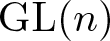
Returning to the question of the extent to which spectrum shrinking entails automatic spectrum preservation, it turns out this is indeed the case even upon restricting the domain of  $\phi$ to
 $GL(n)$,
 $U(n)$, or any number of other topological matrix domains of interest. Corollary 2.2 below provides a sample of possibilities for what those matrix spaces can be:
Theorem 1.1. Let  $m,n\in {\mathbb Z}_{\ge 1}$ and take for
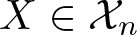
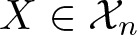
 ${\mathcal X}_n\subseteq M_n$ any one of the following subsets:
•
${\mathcal X}_n=M_n$ or the subset of diagonalizable matrices;•
${\mathcal X}_n=GL(n)$ or the subset of diagonalizable invertible matrices;•
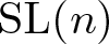
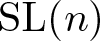
${\mathcal X}_n=SL(n)$ or the subset of diagonalizable determinant-1 matrices;•
${\mathcal X}_n=U(n)$;•
${\mathcal X}_n=N_n$ – the subset of normal
$n\times n$ matrices.


Then there exists a continuous spectrum shrinker
 \begin{equation*}
\phi : {\mathcal X}_n \to M_m
\end{equation*}
if and only if  $n$ divides
 $m$, in which case we have the equality
 \begin{equation*}
k_{\phi(X)}
=
(k_{X})^{\frac mn}
,\quad
\forall X\in {\mathcal X}_n,
\end{equation*}
where  $k_{\bullet}$ denotes the characteristic polynomial of
 $\bullet$.
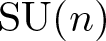
By Remark 2.4, the analogous result fails for the subset  $H_n$ of
 $n\times n$ self-adjoint matrices and the special unitary group
 $SU(n)$,
 $n \geq 2$, as both sets admit a continuous eigenvalue selection.
Section 3 focuses instead on results classifying continuous spectrum-shrinking maps defined on various matrix domains. A paraphrased aggregate of Theorems 3.1 and 3.7 reads as follows.
Theorem 1.2. Let  $n\in {\mathbb Z}_{\ge 3}$ and
 $\phi : {\mathcal X}_n\to M_n$ a continuous, commutativity-preserving and spectrum-shrinking map for a subset
 ${\mathcal X}_n\subseteq M_n$.
If  ${\mathcal{X}}_n\in \{GL(n), SL(n), U(n), N_n\}$ or consists of the diagonalizable matrices in either
 $GL(n)$ or
 $SL(n)$, then
 $\phi$ is either a conjugation or a conjugation composed with transposition.
Our proof of the semisimple branch of Theorem 1.2 does not rely on Šemrl’s theorem A. In fact, a simple continuity argument recovers Theorem A via Theorems 1.1 and 1.2.
The techniques employed in proving Theorems 1.1 and 1.2 involve very little direct computation, being in part algebraic, in part reliant on the topology of the various matrix sets involved, and in part operator-theoretic: in analysing a qualitatively new candidate
 \begin{equation}
SNS^{-1}
\mapsto{\quad}
S^{-1}NS
,\quad
\forall\ \text{normal} N\in N_n\ \text{and positive} S\in GL(n),
\end{equation}
(to show that it in fact meets all of the requirements save for continuity) we make crucial use of the celebrated Putnam–Fuglede theorem [Reference Rosenblum32, Theorem].
There is some hope of extending the main results, and several directions present themselves for doing so: other compact matrix Lie groups in place of  $U(n)$, various infinite-dimensional versions of the results, etc. In part, this forms the object of future work based on adjacent techniques.
2. Leveraging spectrum shrinking into spectrum preservation
To spell out a convenient common generalization, we need some notation.
First of all, by  ${\mathbb C}^{\times}$ we denote the group of non-zero complex numbers. Now let
 $n \in {\mathbb Z}_{\ge 1}$. As usual, we identify vectors in
 ${{\mathbb{C}}}^n$ with the corresponding column-matrices. Similarly, depending on context, we also identify vectors in
 ${{\mathbb{C}}}^n$ with corresponding diagonal matrices and vice versa. For a matrix
 $X \in M_n$ we denote by
 $k_X(x) := \det(x I_n-X)$ its characteristic polynomial (
 $I_n$ is the identity matrix in
 $M_n$). We naturally identify the symmetric group
 $S_n$ with the
 $n \times n$ permutation matrices, so that
 $S_n \leqslant GL(n)$. The convention pertaining to permutations is that
 $\sigma\in S_n\leqslant GL(n)$ operates by
 \begin{equation*}
e_j
\mapsto{\quad\sigma\quad}
e_{\sigma(j)}
,\quad
(e_1, \ldots, e_n)\ \text{the standard basis of}\ {\mathbb C}^n
\end{equation*}
or, equivalently, the left action on (column) size- $n$ vectors is
 \begin{equation}
(x_1, \ldots, x_n)
\mapsto{\quad\sigma\quad}
(x_{\sigma^{-1}(1)}, \ldots , x_{\sigma^{-1}(n)}).
\end{equation}
The symbol  $\text{Ad}_{G}$ denotes the conjugation (or adjoint) action of a subgroup
 $G\leqslant GL(n)$ on
 $M_n$, so that for
 $S \subseteq M_n$,
 \begin{equation*}
\text{Ad}_{G}S=\{gxg^{-1} \ : \ x \in S,\ g \in G\}.
\end{equation*}
Given a subset  $L\subseteq {{\mathbb{C}}}^n$, by
 $\Delta_{L}$ we denote the subset of
 $L$ that consists of elements with at least two equal coordinates:
 \begin{equation*}
\Delta_{L}
:=
\left\{(x_1, \ldots, x_n)\in L \ : \ x_j=x_k\ \text{for some} j\ne k\right\}.
\end{equation*}
If  $V$ is a linear subspace of the algebra
 $T^{+}(n)$ of
 $n \times n$ strictly upper-triangular matrices, denote by
 $T_{L,V} = T_{L,V}(n)$ the set of upper-triangular matrices with diagonal in
 $L$ and strictly upper-triangular component in
 $V$:
 \begin{equation*}
T_{L,V}:=\{diag(\lambda_1, \ldots, \lambda_n) + v \ : \ (\lambda_1, \ldots, \lambda_n) \in L, \ v \in V\}.
\end{equation*}
In the statement of Theorem 2.1 below, we refer to the conjugation action of the group  $S_n\leqslant GL(n)$ of permutation matrices on the set
 $L$ of tuples, identified with that of diagonal matrices. Assuming that
 $L$ is invariant under the action of
 $S_n$ in
 ${\mathbb C}^n$,
 $S_n$ will then also act on
 $\Delta_L$, on the complement
 $L\!\setminus\! \Delta_L$ and hence, finally, also on the set of connected components of
 $L\!\setminus\! \Delta_L$.
Theorem 2.1. Let  $n\in {\mathbb Z}_{\ge 1}$,
 $G\leqslant GL(n)$ a closed connected subgroup,
 $V\leqslant T^{+}(n)$ a linear subspace and
 $L\subseteq {\mathbb C}^n$ a subset such that
•
$L\!\setminus\! \Delta_L$ is dense in
$L$;•
$L$ is invariant under the action of
$S_n$ in
${\mathbb C}^n$;• and the isotropy groups of the connected components of
$L\!\setminus\! \Delta_L$ in
$G\cap S_n$ are transitive on
$\{1,2,\ldots,n\}$.


Then for an arbitrary  $m\in {\mathbb Z}_{\ge 1}$ there exists a continuous spectrum shrinker
 \begin{equation*}
\phi : \text{Ad}_{G}T_{L,V} \to M_m
\end{equation*}
if and only if  $n$ divides
 $m$ and in that case we have the equality of characteristic polynomials
 \begin{equation}
k_{\phi(X)}
=
(k_{X})^{\frac mn}
,\quad
\forall X\in \text{Ad}_{G}T_{L,V}.
\end{equation}
The proof of Theorem 2.1 is (perhaps surprisingly) both elementary and short; we provide it below, after first recording a number of specializations to matrix domains that are naturally of interest. For a subset  $M \subseteq M_n$ we write
 $M_{ss}\subseteq M$ for the subset of semisimple (i.e., diagonalizable) matrices therein.
Corollary 2.2. The conclusion of Theorem 2.1 holds for continuous spectrum-shrinking maps  $\phi : {\mathcal X}_n\to M_m$ in any of the following cases.
(a)
${\mathcal X}_n=M_n$ or
$(M_{n})_{ss}$;(b)
${\mathcal X}_n=GL(n)$ or
$GL(n)_{ss}$;(c)
${\mathcal X}_n=SL(n)$ or
$SL(n)_{ss}$;(d)
${\mathcal X}_n=U(n)$;(e)
${\mathcal X}_n=N_n$.


Proof. This is a simple matter of specifying how to fit the various cases into the framework of Theorem 2.1 by setting the parameters  $G$,
 $L$ and
 $V$.
(I) The group
$G$. For (a), (b) and (c) it is
$G:=GL(n)$, while in the other two cases it is
$G:=U(n)$.(II) The subspace
$V\leqslant T^{+}(n)$. All of
$T^{+}(n)$ in (a), (b) and (c) for arbitrary (as opposed to semisimple) matrices, and
$V:=\{0\}$ in all other cases.(III) The subset
$L\subseteq {\mathbb C}^n$. It is
$L:={\mathbb C}^n$ in (a),
$({\mathbb C}^{\times})^n$ in (b),
\begin{equation*}
\left\{(\lambda_1, \ldots, \lambda_n)\in {\mathbb C}^n\ :\ \prod_{j=1}^n \lambda_j=1\right\}
\text{in (c)},
\end{equation*}
$({\mathbb S}^1)^n$ in (d) and again
${\mathbb C}^n$ in (e).


In cases (a), (b), (c) and (e), where  $L$ is a connected complex algebraic variety and
 $\Delta_L$ a closed algebraic subset thereof, the complement
 $L\!\setminus\! \Delta_L$ is connected [Reference Cooper and Manning9, Proposition 8.3] so there is nothing further to check with regard to the transitivity hypothesis.
In case (d),  $L\!\setminus\!\Delta_L$ is precisely the
 $n$th configuration space [Reference Ghrist12, Definition 1.1]
 ${\mathcal C}^n({\mathbb S}^1)$ consisting of
 $n$-tuples of distinct modulus-
 $1$ complex numbers. As we will see in Lemma 2.3,
 ${\mathcal C}^n({\mathbb S}^1)$ is disconnected as soon as
 $n\ge 3$. The same result, however, shows that the isotropy groups of the connected components are the (transitive) conjugates of the subgroup generated by the cycle
 $(1\ 2\ \cdots\ n)$.
In the following statement, we denote by  $\langle{\eta}\rangle$ the cyclic subgroup generated by an element
 $\eta\in S_n$ and by
 $\pi_0(X)$ the space of components of a topological space
 $X$; the space
 $X={\mathcal C}^n({\mathbb S}^1)$ we are concerned with being a manifold, components and path components coincide [Reference Lee22, Propositions 4.23 and 4.26].
Lemma 2.3. Let  $n\in {\mathbb Z}_{\ge 1}$. The symmetric group
 $S_n$ acts transitively on the space
 $\pi_0({\mathcal C}^n({\mathbb S}^1))$ of components of the circle’s
 $n$th configuration space, and the isotropy groups are the conjugates
 \begin{equation*}
g\langle{\eta}\rangle g^{-1}\leqslant S_n
,\quad
g\in S_n
,\quad
\eta:=(1\ 2\ \cdots\ n).
\end{equation*}
Proof. Consider  $n$ distinct points
 $z_1, \ldots,z_n\in {\mathbb S}^1$. Traversing the circle counterclockwise will enumerate the points as
 \begin{equation*}
z_{\tau(1)},\ z_{\tau(2)},\ldots, z_{\tau(n)}
\end{equation*}
for some permutation  $\tau$, uniquely determined up to right multiplication by powers of
 $\eta$. Associating the class of
 $\tau$ in
 $S_n/\langle{\eta}\rangle$ to the component in question provides a map
 $${\pi _0}({\mathcal{C}^n}({\mathbb{S}^1}))\overrightarrow {\quad {\text{equivariant for the}}\;{S_n} - {\text{actions on the (co)domain }} } \quad {S_n}/\langle \eta \rangle.$$
That map is surjective because the  $S_n$-action on its codomain
 $S_n/\langle{\eta}\rangle$ is transitive, and the conclusion will follow once we observe that (2.3) is also injective.
It will suffice to prove that the preimage of  $\langle{\eta}\rangle\in S_n/\langle{\eta}\rangle$ is a singleton (the argument is not materially different for other cosets). In other words, the goal is to show that
 \begin{equation}
\left\{
(z_1, \ldots, z_n)\in {\mathcal C}^n({\mathbb S}^1)\ :\ z_j\ \text{are ordered counterclockwise increasingly with}\ j
\right\}
\end{equation}
is (path-)connected. To that end, note that a counterclockwise rotation allows us to assume  $z_1=1\in {\mathbb S}^1$, and the resulting subset of (2.4) is
 \begin{equation*}\left\{\left(\exp(2\pi ix_1),\;\dots,\;\exp(2\pi ix_n)\right)\;:\;0=x_1\leq\;x_2\leq\cdots\leq\;x_n \lt \;1\right\}.\end{equation*}
This is the image through the continuous map  \[{\mathbb{R}^n}\underrightarrow {\quad \exp {{(2\pi i \bullet )}^n}\quad }{({\mathbb{S}^1})^n}\] of the (path-connected) interior of an
 $(n-1)$-simplex.
Remarks 2.4.
(1) If
$m=rn$ for some
$r \in {{\mathbb{Z}}}_{\ge 1}$, then an apparent class of continuous maps
$\phi : \mathcal{X}_n \to M_m=M_r(M_n)$ which satisfy (2.2) is given by
where
\begin{equation*}
\phi(X)=S(X) \begin{pmatrix} X \otimes I_p & 0 \\ 0 & X^t \otimes I_q\end{pmatrix} S(X)^{-1},
\end{equation*}
$S:{\mathcal{X}}_n \to GL(m)$ is a continuous function and
$p,q \in {{\mathbb{Z}}}_{\ge 0}$ are such that
$p+q=r$.(2) The ‘obvious analogue’ of Corollary 2.2 does not hold for the corresponding maps
$\phi : H_n \to M_m$ defined on the real subspace
$H_n$ of
$n \times n$ self-adjoint matrices, as for any
$m \in {\mathbb Z}_{\ge 1}$ we can define
$\phi(X):=\lambda_{\max}(X) I_m$, where
$\lambda_{\max}(X)$ denotes the largest eigenvalue of
$X\in H_n$ (which continuously depends on
$X$).(3) An analogous remark applies to
${\mathcal X}_n:=SU(n)$, the special unitary group: Corollary 2.2 does not hold for it, because for any
$n \in {\mathbb Z}_{\ge 1}$ there exists a continuous eigenvalue selection
$\varphi : SU(n) \to {\mathbb S}^1$. As before, for any
$m \in {\mathbb Z}_{\ge 1}$ the assignment
$X \mapsto \varphi(X)I_m$ defines a continuous, commutativity-preserving and spectrum-shrinking map
$SU(n) \to M_m$.To see that there is a continuous eigenvalue selection
$SU(n)\to {\mathbb S}^1$, first identify (per [Reference Bröcker and tom Dieck3, Proposition IV.2.6]) the space
$SU(n)/\text{Ad}_{SU(n)}$ of conjugacy classes with the quotient
${\mathbb T}/S_n$ of the maximal torus
by the Weyl group
\begin{equation*}
{\mathbb T}:=\left\{(\lambda_1, \ldots, \lambda_n)\in \left({\mathbb S}^1\right)^n\ :\ \prod_{j=1}^n \lambda_j=1\right\}
\end{equation*}
$S_n$ of
$SU(n)$ [Reference Bröcker and tom Dieck3, Theorem IV.3.3]. Further, [Reference Morton24, Lemmas 1 and 2] show that
implements a homeomorphism between
\begin{equation*}
(x_1,\ldots, x_n)
\mapsto{\quad}
\left(\exp(2\pi i x_1),\ldots, \exp(2\pi i x_n)\right)
\end{equation*}and
\begin{equation*}
F:=\left\{(x_1, \ldots, x_n)\in {\mathbb R}^n\ :\ \sum_{j=1}^n x_j=0,\ x_1\leqslant x_2\leqslant \cdots\leqslant x_n\leqslant x_1+1\right\}
\end{equation*}
${\mathbb T}/S_n$. We can now simply take our continuous eigenvalue selection to be
\begin{equation*}
SU(n)
\twoheadrightarrow SU(n)/\text{Ad}_{SU(n)}
\cong
{\mathbb T}/S_n
\cong
F
\ni
(x_1, \ldots, x_n)
\mapsto{\quad}
\exp(2\pi i x_1)
\in {\mathbb S}^1.
\end{equation*}


One consequence of Corollary 2.2 is a generalization of the well-known fact that for  $n \geq 2$ there is no (global) continuous selection of eigenvalues of matrices in
 $M_n$ (i.e., there does not exist a continuous map
 $\phi : M_n\to {{\mathbb{C}}}$ such that
 $\phi(X) \in sp(X)$ for all
 $X \in M_n$, see e.g., [Reference Chi-Kwong and Zhang8, Example 2] and Proposition 2.9 below for a more elaborate statement):
Corollary 2.5. Let  $m,n \in {\mathbb Z}_{\ge 1}$ and let
 $\mathcal{X}_n$ be any one of the matrix domains of Corollary 2.2.
(a) If
$n$ does not divide
$m$, there does not exist a continuous spectrum-shrinking map
$\phi: \mathcal{X}_n\to M_m$.(b) If
$n$ divides
$m$, then any continuous spectrum-shrinking map
$\phi: \mathcal{X}_n\to M_m$ is in fact a spectrum preserver.


The second direct consequence is the following strengthening of Theorem A:
Corollary 2.6. Let  $\phi : M_n \to M_n, n \ge 3$, be a continuous commutativity-preserving and spectrum-shrinking map. Then there exists
 $T \in\mathrm{GL}(n)$ such that
 $\phi$ is of the form (1.1).
As noted after the statement of Theorem 1.2, we also obtain an independent proof of Corollary 2.6, not relying on Theorem A.
In the proofs of Theorems 2.1 and 3.1, we shall use the following simple lemma:
Lemma 2.7. Let  $X$ and
 $Y$ be topological spaces such that
 $X$ is connected and
 $Y$ is Hausdorff. Let
 $n\in {\mathbb Z}_{\ge 1}$ and suppose that
 $g,f_1,\ldots,f_n : X \to Y$ are continuous functions such that for each
 $x \in X$ we have
•
$g(x) \in \{f_1(x),\ldots,f_n(x)\}$,•
$f_j(x) \ne f_k(x)$ for all
$1 \leqslant j \ne k \leqslant n$ and all
$x\in X$.


Then there exists  $1 \leqslant j \leqslant n$ such that
 $g=f_j$.
Proof. The sets  $\{x \in X : g(x) = f_1(x)\},\ldots, \{x \in X : g(x) = f_n(x)\}$ are closed and form a partition of
 $X$. By the connectedness of
 $X$, exactly one of them is non-empty and hence equal to all of
 $X$.
Proof of Theorem 2.1
The ‘if’ part of the theorem is covered by Remark 2.4(1).
Denote by  ${\mathbb C}_{\leqslant m}[x]$ the space of complex polynomials of degree
 $\leqslant m$, equipped with the unique Hausdorff linear topology, compatible with that of
 ${\mathbb C}$. The function
 $${\text{A}}{{\text{d}}_G}{T_{L,V}}\underrightarrow {\quad {k_{\phi ( \cdot )\quad }}}{\mathbb{C}_{m}}[x]$$
is continuous, and on an element with spectrum  $(\lambda_1, \ldots, \lambda_n)$ takes one of the finitely many values
 $\prod_{j=1}^n (x-\lambda_j)^{k_j}$ for non-negative integers
 $k_1, \ldots, k_n$ with sum
 $m$. It is enough to prove the claimed equality (2.2) for matrices of the form
 \begin{equation}
T=g \left(diag(\lambda_1, \ldots, \lambda_n)+v\right)g^{-1}
,\quad
g\in G,\ (\lambda_1, \ldots, \lambda_n) \in L':=L\!\setminus\!\Delta_L,\ v\in V,
\end{equation}
as such matrices (whose eigenvalues are all distinct) form a dense subset of  $\text{Ad}_{G}T_{L,V}$. By Lemma 2.7 for
 $T$ as in (2.5) the characteristic polynomial
 $k_{\phi(T)}$ depends only on
 $(\lambda_1, \ldots, \lambda_n)\in L'$:
 $g$ and
 $v$ range over the (path-)connected spaces
 $G$ and
 $V$, respectively. Furthermore, by the selfsame Lemma 2.7, for every connected component
 $L'_0$ of
 $L'$ we have
 \begin{equation}
k_{\phi(diag(\lambda_1, \ldots, \lambda_n))}
=
\prod_{j=1}^n (x-\lambda_j)^{k_{j,L'_0}},
\quad
\forall (\lambda_1, \ldots, \lambda_n)\in L'_0.
\end{equation}
Now, because we are furthermore assuming the isotropy group of  $L'_0$ in
 $S_n\cap G$ is transitive and
 $k_{\phi(\cdot)}$ is invariant under
 $G$-conjugation, the exponents of (2.6) must in fact all be equal. Indeed, consider
 $1\leqslant \ell \lt \ell'\leqslant n$ and
 $\sigma \in S_n\cap G$ fixing
 $L'_0$ with
 $\sigma(\ell)=\ell'$. We then have
 \begin{equation*}
\begin{aligned}
(x-\lambda_{\ell'})^{k_{\ell',L'_0}}
\cdot
\prod_{j\ne \ell'}^n (x-\lambda_j)^{k_{j,L'_0}}
&=
\prod_{j=1}^n (x-\lambda_j)^{k_{j,L'_0}}\\
&=
k_{\phi(diag(\lambda_1, \ldots, \lambda_n))}
\quad\text{by (2.6)}\\
&=
k_{\phi(\sigma^{-1} diag(\lambda_1, \ldots, \lambda_n)\sigma)}
\quad\text{by the G-invariance of}\ k_{\phi(\cdot)}\\
&=
k_{\phi(diag(\lambda_{\sigma(1)}, \ldots, \lambda_{\sigma(n)}))}
\quad\text{by (2.1)}\\
&=
\prod_{j=1}^n \left(x-\lambda_{\sigma(j)}\right)^{k_{j,L'_0}}
\quad\text{by}\,\, (2.6)\ \text{again, because}\ \sigma\ \text{fixes}\ L'_0\\
&=
(x-\lambda_{\ell'})^{k_{\ell,L'_0}}
\cdot
\prod_{j\ne \ell}^n (x-\lambda_{\sigma(j)})^{k_{j,L'_0}}
\end{aligned}
\end{equation*}
and hence  $k_{\ell',L'_0} = k_{\ell,L'_0}$. Thus, for each connected component
 $L'_0$ of
 $L'$, all exponents
 $k_{j,L'_0}$ are equal. Denote their common value by
 $r_{L'_0}$. Since
 $\sum_{j=1}^n k_{j,L'_0}=m$, we have
 $m=nr_{L'_0}$. In particular,
 $n$ divides
 $m$, and necessarily
 $r_{L'_0}=m/n$, independently of
 $L'_0$. Therefore, for every matrix
 $T$ of the form (2.5),
 \begin{equation*}
k_{\phi(T)}
=
\prod_{j=1}^n (x-\lambda_j)^{\frac{m}{n}}
=
\left(\prod_{j=1}^n (x-\lambda_j)\right)^{\frac{m}{n}}
=
(k_T)^{\frac{m}{n}}.
\end{equation*}
Such matrices form a dense subset of  $\text{Ad}_{G}T_{L,V}$, and both sides depend continuously on
 $T$. Hence (2.2) holds on all of
 $\text{Ad}_{G}T_{L,V}$.
Remarks 2.8.
An essential feature of  ${\mathcal{X}}_n$ in Corollary 2.2 is the non-existence of a continuous eigenvalue selection
 ${\mathcal{X}}_n \to {{\mathbb{C}}}$.
(1) Even though Corollary 2.2 holds for
${\mathcal{X}}_n = U(n)$, it does not hold for any of its open dense subsets
where
\begin{equation*}
U(n)_{\lambda}:=\{X \in U(n) \ : \ \lambda \notin sp(X)\},
\end{equation*}
$\lambda \in {\mathbb S}^1$. Indeed, for each
$X \in U(n)_{\lambda}$ choose
$\varphi(X) \in sp(X)$ with the largest value of the corresponding (continuous) branch of the argument, defined on
${{\mathbb{C}}}\setminus \{t\lambda : t \geq 0\}$. Then as before, if
$n \geq 2$, the assignment
$U(n)_{\lambda} \to M_m$,
$X \mapsto \varphi(X)I_m$, defines a continuous proper spectrum shrinker. In particular, as
$\{U(n)_\lambda \ : \ \lambda \in {\mathbb S}^1\}$ forms an open cover of
$U(n)$, any unitary matrix admits a local continuous eigenvalue selection.(2) Fix any norm
${{\left\| \cdot \right\|}}$ on
$M_n$. If
${\mathcal{X}}_n\in \{M_n, GL(n)\}$, we can slightly strengthen the statement of Corollary 2.2 for maps defined on
$B_{{{\left\| \cdot \right\|}}}(0_n,r)\cap {\mathcal{X}}_n$, for any
$r \gt 0$ (instead of the whole
${\mathcal{X}}_n$). Indeed, if
$\psi : B_{{{\left\| \cdot \right\|}}}(0_n,r)\cap {\mathcal{X}}_n \to M_m$ is a continuous spectrum-shrinking map, then this follows by applying Corollary 2.2 to the map
which satisfies the same properties.
\begin{equation*}\phi : {\mathcal{X}}_n \to M_m, \qquad \phi(X) := \frac{1+{{\left\| X \right\|}}}{r}\psi\left(\frac{r X}{1+{{\left\| X \right\|}}}\right),\end{equation*}


Remark 2.8(2) implies that no neighbourhood of  $0_n\in M_n$ admits a continuous eigenvalue selector (by contrast to the parallel situation in
 $U(n)$, per Remark 2.8(1)). The following result answers the natural question of which matrices share this property.
Proposition 2.9. Let  $n\in {\mathbb Z}_{\ge 1}$. A matrix in either
 $M_n$ or
 $GL(n)$ has a neighbourhood admitting a continuous eigenvalue selection if and only if it has at least one simple eigenvalue.
Proof. The statement for  $M_n$ will of course recover that for
 $GL(n)$, the latter being an open subset of the former. We thus focus on
 $M_n$.
(i)
$(\Leftarrow)$ Suppose
$\lambda$ is a simple spectrum point for
$X\in M_n$. By the continuity of both characteristic polynomials and spectra [Reference Newburgh25, Theorem 3], for small
$\varepsilon \gt 0$ and a sufficiently small neighbourhood
${\mathcal U}\ni X$ in
$M_n$ every
$Y\in {\mathcal U}$ has a unique eigenvalue
\begin{equation*}
\lambda_Y
\in
\left\{z\in {\mathbb C}\ :\ |z-\lambda| \lt \varepsilon\right\}.
\end{equation*}This provides us with the desired (plainly continuous) selector:
$Y\mapsto \lambda_Y$ for
$Y\in {\mathcal U}$.(ii)
$(\Rightarrow)$ Assume now that all spectrum points of
$X\in M_n$ have algebraic multiplicity
$\ge 2$, and that we have a continuous eigenvalue selector
\begin{equation*}
{\mathcal U}\ni Y
\mapsto{\quad}
\lambda_Y
\in {\mathbb C}
,\quad
{\mathcal U}\ni X\text{a neighbourhood}.
\end{equation*}Restricting attention to matrices leaving invariant the (at least two-dimensional, by assumption) generalized
$\lambda$-eigenspace [Reference Bronson5, § 9.4]
of
\begin{equation*}
\bigcup_{m\in {\mathbb Z}_{\ge 0}}\ker\left(\lambda I_n-X\right)^m
\end{equation*}
$X$, we can assume the spectrum
$sp(X)$ is a singleton. Translation by
$\lambda I_n\in M_n$ further reduces the problem to nilpotent operators
$X$. Because moreover every neighbourhood of a nilpotent operator contains another such with a single Jordan block [Reference Horn and Johnson18, Definition 3.1.1], conjugation turns the problem into its instance for
\begin{equation*}
X
:=
J_n(0)
:=
\begin{pmatrix}
0&1&\phantom{-}&\phantom{-}&\phantom{-}\\
\phantom{-}&0&1&\phantom{-}&\phantom{-}\\
\phantom{-}&\phantom{-}&\ddots&\ddots&\phantom{-}\\
\phantom{-}&\phantom{-}&\phantom{-}&0&1\\
\phantom{-}&\phantom{-}&\phantom{-}&\phantom{-}&0
\end{pmatrix}.
\end{equation*}This case, in turn, is easily handled as in [Reference Chi-Kwong and Zhang8, Example 2] (the current problem’s version for
$n=2$): for any neighbourhood
${\mathcal U}\ni 0$ in
${\mathbb C}$, the
$z$-dependent matrix
with characteristic polynomial
\begin{equation*}
X_z
:=
\begin{pmatrix}
0&1&\phantom{-}&\phantom{-}&\phantom{-}\\
\phantom{-}&0&1&\phantom{-}&\phantom{-}\\
\phantom{-}&\phantom{-}&\ddots&\ddots&\phantom{-}\\
\phantom{-}&\phantom{-}&\phantom{-}&0&1\\
z&\phantom{-}&\phantom{-}&\phantom{-}&0
\end{pmatrix}
\end{equation*}
$x^n\pm z$ does not admit a continuous eigenvalue selector.


3. Classification results
One of the present section’s main results is the following preserver result:
Theorem 3.1. Let  ${\mathcal{X}}_n\in \{GL(n), SL(n), U(n), N_n\}$,
 $n \geq 3$ and
 $\phi : {\mathcal{X}}_n \to M_n$ a continuous commutativity-preserving and spectrum-shrinking map.
There exists  $T \in GL(n)$ such that
 $\phi$ is of the form (1.1).
We gather some auxiliary remarks and results building up to a proof of Theorem 3.1. Proposition 3.2 is essentially a variant of [Reference Šemrl36, Lemma 2.1] applicable to either algebraic or unitary tori, i.e.,  $({\mathbb C}^{\times})^n$ or
 $({\mathbb S}^1)^n$ respectively. The proof of the aforementioned result adapts easily to arbitrary (as opposed to unitary) invertible matrices, but we provide a short alternative in that case as well for completeness.
Proposition 3.2. For  $n\in {\mathbb Z}_{\ge 1}$ denote by
 $G\leqslant GL(n)$ the group of arbitrary, determinant-1, or unitary diagonal matrices.
A continuous commutativity- and spectrum-preserving map  $\phi : G \to GL(n)$ is conjugation by some
 $T\in GL(n)$.
Proof. Consider a fixed diagonal matrix  $X=diag(x_1, \ldots, x_n)\in G$ with distinct eigenvalues
 $x_j$. Its image
 $\phi(X)$ is a conjugate thereof (by spectrum preservation), so we may as well assume
 $\phi(X)=X$ for simplicity (and hence
 $\phi(G)$ consists of diagonal matrices by commutativity preservation). It follows that
 $\phi(Y)$ simply permutes the entries of
 $Y$ for any
 $Y\in G$ with distinct eigenvalues:
 \begin{equation*}
\left(\forall Y=diag(y_1, \ldots, y_n)\in G\right)
\left(\exists \tau\in S_n\right)
\quad:\quad
\phi(Y) = diag(y_{\tau(1)},\ldots, y_{\tau(n)}).
\end{equation*}
As before, we identify the groups of invertible diagonal and unitary diagonal matrices in  $GL(n)$ with
 $({\mathbb C}^{\times})^n$ and
 $({\mathbb S}^1)^n$, respectively.
(i)
$G=({\mathbb C}^{\times})^n$ or the determinant-1 tuples therein. That
$\tau$ is the identity for all
$Y\in G$ with distinct eigenvalues follows from: the continuity of
$\phi$, the fact that the space of simple-spectrum elements of
$G$ is connected (per [Reference Cooper and Manning9, Proposition 8.3], as remarked in the proof of Corollary 2.2), Lemma 2.7, and the density of such matrices
$Y$ in
$G$.(ii)
$G=({\mathbb S}^1)^n$. By Lemma 2.3,
${\mathcal C}^n({\mathbb S}^1)$ is connected only for
$n=1,2$, when the preceding argument applies; we henceforth assume
$n \geq 3$. What Lemma 2.7 still delivers is a map sending a component
$C\in \pi_0({\mathcal C}^n({\mathbb S}^1))$ to the permutation
$\tau=\tau_C\in S_n$ satisfying
and hence a function
\begin{equation*}
\phi(Y) = diag(y_{\tau(1)},\ldots, y_{\tau(n)})
,\quad
\forall Y\in C,
\end{equation*}Fix a transposition
$\sigma=(j\ j')$ and consider convergent tuple sequences
for a connected component
\begin{equation*}
C
\supset
\textbf{y}_m=(y_{m,i})_{i=1}^n
\mathrel{\mathop{\longrightarrow}\limits_{\quad{m \quad}}}{}
\textbf{y}=(y_i)_i
\mathrel{\mathop{\longleftarrow}\limits_{\quad{m \quad}}}{}
\sigma\textbf{y}_m=(y_{m,\sigma^{-1}(i)})_{i=1}^n
\subset
C'
:=
\sigma C
\end{equation*}
$C$ of
${\mathcal C}^n({\mathbb S}^1)$, with the common limit
having a single equality between two components (necessarily the
\begin{equation*}
\textbf{y}\in \overline{C}\cap \overline{C'}\subseteq ({\mathbb S}^1)^n
\end{equation*}
$j$th and
$(j')$th). Writing
$\tau:=\tau_C$ and
$\tau':=\tau_{C'}$, we have
\begin{equation*}
(y_{\tau(i)})_i = (y_{\sigma\tau'(i)})_i
\ \Longrightarrow{\quad}\
y_{\ell} = y_{\sigma\tau'\tau^{-1}(\ell)}
,\quad \forall 1\leqslant \ell\leqslant n
\ \Longrightarrow{\quad}\
\tau'\in \left\{\tau,\ \sigma\tau\right\}.
\end{equation*}The above assumptions impose some constraints on
$C$ and
$\sigma=(j\ j')$: elements of
$C$ can converge to
$\mathbf{y}$ with a single coordinate equality only when that equality is between two entries of
$\mathbf{y}$ consecutive in a counterclockwise ordering around the circle: if
are the respective counterclockwise orderings of the tuples
\begin{equation*}
y_{m,\tau(1)}
,\quad
y_{m,\tau(2)}
,\quad
\cdots
,\quad
y_{m,\tau(n)}
\end{equation*}
$\mathbf{y}_{m}\in C$, then those of the
$\sigma \mathbf{y}_m$ must be obtained from the former by interchanging two indices
$\tau(k)$ and
$\tau(k+1)$ for some
$k\in \left\{1,\ldots, n\right\}$ (identifying
$n+1=1$). In other words, if
$C$ corresponds via (2.3) to
$\tau$, then
$\sigma$ must be of the form
$\tau (k\ k+1)\tau^{-1}$ for a simple transposition
$(k\ k+1)$; in conclusion:
(3.1)\begin{equation}
\left(\forall \theta\in S_n\right)
\left(\forall\ \text{simple transposition} \sigma\in S_n\right)
\quad:\quad
\tau_{\theta\sigma}
=
\tau_{\theta\sigma\theta^{-1}\cdot\theta}
\in
\left\{\tau_{\theta},\ \theta\sigma\theta^{-1}\tau_{\theta}\right\}.
\end{equation}We claim that in fact only the first listed option occurs:
(3.2)\begin{equation}
\left(\forall \theta\in S_n\right)
\left(\forall\ \text{simple transposition} \sigma\in S_n\right)
\quad:\quad
\tau_{\theta\sigma}
=
\tau_{\theta\sigma\theta^{-1}\cdot\theta}
=
\tau_{\theta}.
\end{equation}Note first that this would indeed finish the proof that
$\tau_{\bullet}$ is constant, for the simple transpositions generate
$S_n$. It thus remains to prove (3.2). Recalling that
$\tau_{\bullet}$ is constant on the left cosets of
$\langle{\eta:=(1\ 2\ \cdots\ n)}\rangle$, we have
$\tau_{\theta}=\tau_{\theta\eta}$. Next, decompose
(3.3)for\begin{equation}
\theta\eta
=
\theta (1\ 2)\cdots (n-1\ n)
=
\sigma_{n-1}\cdot \sigma_{n-2}\cdots \sigma_1\cdot \theta
\end{equation}
$\sigma_j$ defined recursively by
\begin{equation*}
\sigma_1:=\theta(1\ 2)\theta^{-1}=\text{Ad}_{\theta}(1\ 2)
,\quad
\sigma_j:=\text{Ad}_{\sigma_{j-1}\cdots \sigma_1\cdot \theta}(j\ j+1).
\end{equation*}By (3.1) we have
and hence
\begin{equation*}
\forall j\in \left\{1,\ldots, n-1\right\}
\quad:\quad
\tau_{\sigma_j\cdots \sigma_1\cdot\theta}
\in
\left\{
\tau_{\sigma_{j-1}\cdots \sigma_1\cdot\theta}
,\
\sigma_j \cdot \tau_{\sigma_{j-1}\cdots \sigma_1\cdot\theta}
\right\},
\end{equation*}for some possibly-empty set of indices
\begin{equation*}
\tau_{\theta\eta}
=
\tau_{\sigma_{n-1}\cdot \sigma_{n-2}\cdots \sigma_1\cdot \theta}
=
\sigma_{j_k}\cdot \sigma_{j_{k-1}}\cdots \sigma_{j_1}\cdot \tau_{\theta}
\end{equation*}
$j_k \gt \cdots \gt j_1$. As no non-empty product
can be trivial, the permutations
\begin{equation*}
\sigma_{j_k}\cdot \sigma_{j_{k-1}}\cdots \sigma_{j_1}
,\quad
j_k \gt \cdots \gt j_1
\end{equation*}must in fact all be equal; in particular,
\begin{equation*}
\tau_{\sigma_j\cdots \sigma_1\cdot\theta}
,\quad
j\in \{0,\ldots ,n-1\}
\end{equation*}
\begin{equation*}
\tau_{\sigma_1\theta} = \tau_{\theta(1\ 2)}=\tau_{\theta}.
\end{equation*}That the same conclusion holds for all
$(j\ j+1)$ in place of
$(1\ 2)$ follows in precisely identical fashion: in (3.3) simply decompose
$\eta$ as
in place of the original
\begin{equation*}
\eta = (j\ j+1) (j+1\ j+2)\cdots (n-1\ n)(n\ 1)\cdots
\end{equation*}
$(1\ 2)\cdots (n-1\ n)$.


We also recast [Reference Šemrl36, Lemma 2.4] in a form suitable for work with normal or unitary operators. We denote by  ${\mathbb G}={\mathbb G} V$ the Grassmannian of the ambient space
 $V:={\mathbb C}^n$ of column vectors on which the algebra
 $M_n$ acts: the collection of all of its subspaces, topologized as
 \begin{equation*}
{\mathbb G} V=\coprod_{0\leqslant d\leqslant n}{\mathbb G}\big(d,V\big)
,\
{\mathbb G}\big(d,V\big):=\left\{d-\text{dimensional subspaces of}\ V\right\}\
\text{[23, Example 1.36]}.
\end{equation*}
Furthermore, we equip the space  $V={{\mathbb{C}}}^n$ with its standard inner product. For a subspace
 $W \in {\mathbb G}$ by
 $P_W$ we denote the orthogonal projection onto
 $W$.
Lemma 3.3. Let  $n\in {{\mathbb{Z}}}_{\ge 1}$ and
 $\phi: U(n) \to GL(n)$ a continuous commutativity- and spectrum-preserving map. The assignment
 $\Psi : {\mathbb G} \to {\mathbb G}$ given by
 \begin{equation}
\psi(W) := \ker(\lambda
I_n-\phi(U)), = \text{for any}\ \lambda \in {\mathbb S}^1 \text{and}\ U\in U(n)\ \text{with} \ker(\lambda I_n-U)=W,
\end{equation}
is a well-defined continuous map which preserves both dimensions and inclusion relations.
Proof. Fix a subspace  $W \leqslant {{\mathbb{C}}}^n$ and consider the unitary operator
 \begin{equation*}
U_W :=2P_W-I_n= id_W \oplus \,(-id_{W^\perp}) \in U(n).
\end{equation*}
Suppose that  $U \in U(n)$ and
 $\lambda\in {\mathbb S}^1$ satisfy
 \begin{equation*}
\ker(\lambda I_n - U) = W.
\end{equation*}
To show that  $\Psi$ is well-defined, it suffices to show
 \begin{equation}
\ker(\lambda I_n - \phi(U)) = \ker(I_n - \phi(U_W)).
\end{equation}
Indeed, let  $S \in U(n)$ be a unitary matrix whose columns consist of the orthonormal eigenbasis for
 $U$. It easily follows that
 \begin{equation*}
U, U_W \in S({\mathbb S}^1)^nS^*.
\end{equation*}
Proposition 3.2 applied to the maximal torus  $G:=S({\mathbb S}^1)^nS^*$ implies that there exists
 $T_{G} \in GL(n)$ such that
 \begin{equation*}
\phi(X) = T_{G} X T_{G}^{-1}
,\quad
\forall
X\in G.
\end{equation*}
In particular, we have
 \begin{align*}
\phi(U) = T_{G} UT_{G}^{-1} {\implies} \ker(\lambda I_n-\phi(U)) & = \ker (T_{G}(\lambda I_n - U)T_{G}^{-1}) = T_{G}(\ker(\lambda I_n - U)) \\
&= T_{G} W.
\end{align*}
Exactly the same calculation gives  $\ker(I_n-\phi(U_W)) = T_{G} W$ which yields (3.5), so that
 \begin{equation}
\Psi(W)=
\ker(I_n-\phi(U_{W}))=T_{G} W.
\end{equation}
That  $\Psi$ preserves dimensions follows from the map’s expression (3.6), as does inclusion preservation: whenever
 $W\leqslant W'$ there is a maximal torus
 $G$ in
 $U(n)$ containing both
 $U_W$ and
 $U_{W'}$, so that
 $\Psi(W)=T_{G} W\leqslant T_{G} W'=\Psi(W')$.
It remains to verify the continuity of  $\Psi$. For a fixed
 $0 \leqslant d \leqslant n$ let
 ${\mathcal U}_{d}\subset M_n$ be the collection of diagonalizable matrices
 $X \in M_n$ such that
 $\dim\ker(I_n - X) = d$. It is straightforward to check that the map

is continuous (e.g., [Reference Saltman33, Proposition 13.4]). As  $U_{W} \in {\mathcal U}_{d}$ varies continuously with
 $W \in {\mathbb G}(d,V)$, it follows that
 $\Psi$ is continuous as a composition

of continuous maps.
The map of Lemma 3.3 is somewhat more than dimension-preserving: if  $V$ and
 $W$ are (complex) vector spaces, recall [Reference Faure11, Definition 2.1] that a map
 $\Psi:{\mathbb P} V \to {\mathbb P} W$ is a morphism between projective spaces if
 $\Psi$ respects sums of lines in the following sense:
 \begin{equation}
\ell \leqslant \ell'\bigvee \ell^{\prime\prime}
\Longrightarrow\Psi\ell\leqslant \Psi\ell'\bigvee\Psi\ell^{\prime\prime}
,\quad
\forall \text{lines} \ell,\ \ell',\ \ell^{\prime\prime}\in {\mathbb P} V,
\end{equation}
where ‘ $\bigvee$’ denotes the supremum operation (i.e., sum) in the subspace lattice [Reference Pankov27, § 1.2] of
 $V$. To prove that
 $\Psi$ is a morphism in this sense (or rather restricts to one on
 ${\mathbb P} V\subset {\mathbb G}$), we need a version of the Fundamental Theorem of Projective Geometry (appearing in various guises as [Reference Faure11, Theorem 3.1], [Reference Pankov27, Theorem 2.3], etc.).
For subspaces  $W,W'\leqslant V\cong {\mathbb C}^n$ write
 $W$

 $W'$ to denote the fact that the orthogonal projections
 $P_W$ and
 $P_{W'}$ commute; this is equivalent to the orthogonal complements of
 $W\cap W'$ in
 $W$ and
 $W'$ being orthogonal, or to the fact that there is a maximal torus
 $G\leqslant U(n)$ leaving both
 $W$ and
 $W'$ invariant. Note first:
Lemma 3.4. The map  $\Psi$ of Lemma 3.3 preserves lattice operations for spaces in relation
 .
Proof. This is precisely for the reason just pointed out in defining  , i.e., the existence of
 $G$: for
 $T=T_G$ attached to
 $G$ as in (3.6), we have
 \begin{equation*}
\Psi(W+W')=T(W+W')=TW+TW'=\Psi(W)+\Psi(W').
\end{equation*}
The following result will thus apply to the map  $\Psi$ constructed in Lemma 3.3.
Proposition 3.5. Let  $V$ be an
 $n$-dimensional complex Hilbert space for
 $n \in {\mathbb Z}_{\ge 3}$,
 ${\mathbb G}:={\mathbb G}(V)$ its Grassmannian. Any continuous self-map
 $\Psi: {\mathbb G} \to {\mathbb G}$ that preserves dimensions and lattice operations for spaces in relation
 is induced by an invertible linear or conjugate-linear operator
 $T$ on
 $V$, in the sense that
 \begin{equation*}
\forall W\in {\mathbb G}
\quad:\quad
\Psi(W)=TW.
\end{equation*}
Proof. There are several stages to the proof. First of all, as  $\Psi$ preserves dimensions, it restricts to a self-map
 $\Psi|_{{\mathbb P} V}:{\mathbb P} V \to {\mathbb P} V$.
(I) Conclusion, assuming
$\Psi|_{{\mathbb P} V}$ is a projective space endomorphism. Suppose, in other words, we have proven (3.7). The image
$\Psi({\mathbb P} V)$ of the projective space
${\mathbb P} V\subset {\mathbb G}$ cannot be contained in a line of
${\mathbb P} V$, for by assumption the restriction
$\Psi|_{{\mathbb P} V}$ sends lines through the elements of an orthogonal basis to distinct
$n=\dim V\ge 3$ (even linearly independent) lines. As we are assuming (in the present portion of the proof) that
$\Psi|_{{\mathbb P} V} : {\mathbb P} V \to {\mathbb P} V$ is an endomorphism of
${\mathbb P} V$, it follows from [Reference Faure11, Theorem 3.1] that
$\Psi|_{{\mathbb P} V}$ is implemented by a semilinear endomorphism
$T: V \to V$:
where
\begin{equation*}
\Psi(\ell) =span_{{\mathbb C}}\ T\ell, \quad \forall \ell \in {\mathbb P} V,
\end{equation*}
$T$ is an additive map for which there exists a ring endomorphism
$\alpha\in End({\mathbb C})$ such that
\begin{equation*}
T(\mu v)=\alpha(\mu)Tv,\quad \forall \mu \in {\mathbb C},\ v\in V.
\end{equation*}An arbitrary subspace
$W \in {\mathbb G}(d,V)\subset {\mathbb G}$ (
$1 \leqslant d \leqslant n$) can be decomposed as
$W=\ell_1 \oplus \cdots \oplus \ell_d$ for some mutually orthogonal lines
$\ell_j \in {\mathbb P} V$, so the assumed compatibility with lattice operations under yields
(3.8)\begin{equation}
\Psi(W) = \Psi(\ell_1) + \cdots +\Psi(\ell_d)= span_{{\mathbb C}} TW.
\end{equation}Obviously
$T$ is injective, as
$\Psi({\mathbb P} V)\subseteq {\mathbb P} V$. As (by assumption)
$\Psi$ is continuous, so is
$\alpha$. Indeed (as argued in [Reference Šemrl36, § 3, p. 133]), consider orthogonal non-zero vectors
$v,w\in V$. Lattice compatibility under then implies that the lines
are distinct. In particular,
\begin{equation*}
{\mathbb C} Tv = \Psi({\mathbb C} v)
\quad\text{and}\quad
{\mathbb C} Tw = \Psi({\mathbb C} w)
\end{equation*}
$Tv$ and
$Tw$ are linearly independent. The map
is continuous, and with it
$\alpha$ by the noted linear independence of
$Tv$ and
$Tw$. That continuity forces
$\alpha\in \left\{id,\ \overline{\bullet}\right\}$, so that by (3.8) we have
for
\begin{equation*}
\forall W\in {\mathbb G}
\quad:\quad \Psi(W) = TW,
\end{equation*}
$T$ either in
$GL(V)$ or invertible conjugate-linear.(II)
$\Psi|_{{\mathbb P} V}$ is a projective space endomorphism. The dimension preservation of
$\Psi$ already constrains the nature of possible counterexamples: the assumed compatibility with implies that
$\Psi$ preserves inclusion, so for lines
$\ell$,
$\ell'$ and
$\ell^{\prime\prime}$ with
$\ell\leqslant \ell'\bigvee\ell^{\prime\prime}$ we have
\begin{equation*}
\text{lines} \Psi(\ell),\ \Psi(\ell'),\ \Psi(\ell^{\prime\prime})\leqslant \text{2-plane} \Psi\left(\ell'\bigvee\ell^{\prime\prime}\right).
\end{equation*}All is thus well provided
$\Psi$ is injective on
${\mathbb P} V$ (for in that case, if
$\ell'\ne \ell^{\prime\prime}$, the distinct lines
$\Psi(\ell')$ and
$\Psi(\ell^{\prime\prime})$ would have to span the right-hand 2-plane in the above equation). We can always reduce the problem to the case
$n=3$, as we will: if
$\Psi(\ell)=\Psi(\ell')$ for distinct lines then consider a three-dimensional subspace
$V'\leqslant V$ containing
$\ell\bigvee\ell'$, and substitute•
$V'$ for
$V$;• and
$R\circ\Psi$ for
$\Psi$, where
$R\in GL(V)$ sends
$\Psi(V')$ back to
$V'$ and we identify
$R$ with the operator
$W\mapsto RW$ it induces on
${\mathbb G}$.
Suppose, then, that
$\Psi(\ell)=\Psi(\ell')$ for
$\ell\ne \ell'\in {\mathbb P} V$ and
$\dim V=3$. We claim that in this case
$\Psi$ is constant on all of
${\mathbb P} \pi$, where
$\pi:=\ell\bigvee \ell'$, contradicting the fact that by assumption
$\Psi$ sends orthogonal lines to linearly independent lines. The projective line
${\mathbb P}\pi$ being connected, it will be enough to argue that
(3.9)is open (for it is already closed by the continuity of\begin{equation}
\Psi^{-1}\left(\Psi(\ell)\right)\cap {\mathbb P}\pi
=
\left\{\ell^{\prime\prime}\leqslant \pi\ :\ \Psi(\ell^{\prime\prime})=\Psi(\ell)=\Psi(\ell')\right\}
\subseteq
{\mathbb P}\pi
\end{equation}
$\Psi$, and non-empty because it contains
$\ell$ and
$\ell'$ themselves). Without loss of generality, this amounts to showing that along with
$\ell'$ the set in question contains an entire neighbourhood thereof in
${\mathbb P}\pi$. Write
so that
\begin{equation*}
\pi':=span\left\{\ell',\ \pi^{\perp}\right\},
\end{equation*}
$\pi$
$\pi'$. We proceed in stages.(a) The line
$\ell'$ belongs to the interior of
$\Psi^{-1}(\Psi(\ell))\cap {\mathbb P} \pi'$ regarded as a subspace of
${\mathbb P} \pi'$. Suppose not. There is then a sequence
\begin{equation*}
{\mathbb P} \pi'\!\setminus\! \Psi^{-1}(\Psi(\ell))
\ni
\ell_k\mathrel{\mathop{\longrightarrow}\limits^{\text{convergence in}\mathbb{G}}_{k}} B
\ell'.
\end{equation*}Because by assumption
$\Psi(\ell_k)\ne \Psi(\ell')=\Psi(\ell)$ for all
$k$, we have (as observed earlier in the proof)
\begin{align*}
\forall k\quad:\quad
\Psi\left(\ell_k\bigvee \ell'\right)
&= \Psi(\ell_k)\bigvee \Psi(\ell')
\underline{\underline {\quad \Psi (\ell ') = \Psi (\ell )\quad }}
\Psi(\ell_k)\bigvee \Psi(\ell)
\\
&= \Psi\left(\ell_k\bigvee \ell\right).
\end{align*}Now,
$\ell_k\bigvee\ell'=\pi'$ for all
$k$ on the one hand and
$\ell_k\bigvee\ell\mathrel{\mathop{\longrightarrow}\limits_{k}}{}\pi$ on the other, so
$\Psi(\pi)=\Psi(\pi')$. On the other hand
and we have a contradiction because
$\pi\bigvee\pi'=V$ has dimension
$3$, whereas
$\Psi(\pi)=\Psi(\pi')$ would make
$\Psi(\pi)\bigvee\Psi(\pi')$ a
$2$-plane.(b) The line
$\ell'$ belongs to the interior of (3.9). Simply apply the preceding step with altered parameters:
$\ell'$ is as before, but substitute any
for
\begin{equation*}
\ell^{\prime\prime} \in \Psi^{-1}(\Psi(\ell))\cap {\mathbb P} \pi'\setminus \{\ell'\}
\end{equation*}
$\ell$ and interchange the roles of
$\pi$ and
$\pi'$.


 yields


 then implies that the lines


 implies that


Proof of Theorem 3.1
First of all, by Corollary 2.2,  $\phi$ preserves spectra.
(I)
${\mathcal{X}}_n = \mathrm{GL}(n)$. By the continuity of the spectral radius
$\rho(\cdot)$ on
$M_n$ (see e.g., [Reference Newburgh25, Theorem 3]), the map
is well-defined and continuous. Consider the map
\begin{equation*}
F : M_n \to \mathrm{GL}(n), \qquad F(X):= X + (1+\rho(X))I_n
\end{equation*}
\begin{equation*}\psi : M_n \to M_n, \qquad \psi(X) := \phi(F(X)) - (1 + \rho(X))I_n.\end{equation*}Clearly,
$\psi$ is a well-defined, continuous, commutativity- and spectrum-preserving map. Therefore, Theorem A implies that there exists
$T \in \mathrm{GL}(n)$ such that
$\psi$ is of the form (1.1). By passing to the map
$T^{-1}\phi(\cdot)T$ or
$(T^{-1}\phi(\cdot)T)^t$, without loss of generality, we can assume that
$\psi$ is the identity map on
$M_n$. In particular, we have
(3.10)\begin{equation}
\phi(F(X))=F(X), \quad \forall X \in M_n.
\end{equation}By Proposition 3.2,
$\phi$ operates as conjugation by an invertible matrix on every maximal algebraic torus of
$GL(n)$ (i.e., conjugate of the subgroup
$D(n)\leqslant GL(n)$ of invertible diagonal matrices):
\begin{equation*}
\left(\forall S\in GL(n)\right)
\left(\exists R\in GL(n)\right)
\left(\forall D\in D(n)\right)
\quad:\quad
\phi(SDS^{-1})
=
RSDS^{-1}R^{-1}.
\end{equation*}The consequence [Reference Šemrl36, Corollary 2.2] follows:
(3.11)\begin{equation}
\left(\forall X\in GL(n)\right)
\left(\forall\text{polynomials}\ p\ :\ p(X)\in GL(n)\right)
\quad:\quad
\phi(p(X))=p(\phi(X)).
\end{equation}Now, for a fixed
$X\in GL(n)$ we have
$F(X)=p_X(X)$ for the polynomial
and hence (as
\begin{equation*}
p_X(\lambda):=\lambda+(1+\rho(X)),
\end{equation*}
$\rho(\phi(X))=\rho(X)$)
\begin{align*}
\phi(X)+(1+\rho(X))I_n
&=
p_X(\phi(X))
\overset{\text{(3.11)}}{=}
\phi(p_X(X))
=
\phi(F(X))
\overset{\text{(3.10)}}{=}
F(X)\\
&=
X+(1+\rho(X))I_n.
\end{align*}We are now done:
$\phi(X)=X$, as desired.(II)
${\mathcal{X}}_n = \mathrm{SL}(n)$. Let
${{\mathbb{R}}}_{\leqslant 0}$ denote the set of all non-positive real numbers and let
be the principal branch of the complex
\begin{equation*}
\sqrt[n]{\cdot}: {{\mathbb{C}}}\setminus {{\mathbb{R}}}_{\leqslant 0} \to {{\mathbb{C}}}\setminus{{\mathbb{R}}}_{\leqslant 0}, \qquad \sqrt[n]{z}=\sqrt[n]{|z|}e^{\frac{i Arg z}{n}}
\end{equation*}
$n$-th root (which is a continuous map). Denote
\begin{equation*}
\mathrm{GL}(n)_*:=\left\{X \in \mathrm{GL}(n) \ : \ \det X \notin {{\mathbb{R}}}_{\leqslant 0} \right\}.
\end{equation*}The map
(3.12)is a continuous, spectrum- and commutativity-preserving extension of\begin{equation}
\zeta : \mathrm{GL}(n)_* \to \mathrm{GL}(n)_*, \qquad \zeta(X) = \sqrt[n]{\det X}\cdot \phi\left(\frac1{\sqrt[n]{\det X}} X\right)
\end{equation}
$\phi$ to
$GL(n)_* \supseteq SL(n)$. To repeat Step (1), we first replace the map
$F$ there by
\begin{equation*}
F_*(X):=X+(n+1)(1+\rho(X))I_n.
\end{equation*}We claim that
$F_*(X)\in GL(n)_*$ for all
$X\in M_n$. Indeed, if
$\lambda\in sp(X)$, then
$|\lambda|\leqslant \rho(X)$, and hence
\begin{equation*}
\operatorname{Re}\big((n+1)(1+\rho(X))+\lambda\big)\ge n\rho(X)+n+1,
\qquad
\left|\operatorname{Im}\big((n+1)(1+\rho(X))+\lambda\big)\right|\leqslant \rho(X).
\end{equation*}Therefore
\begin{equation*}
\left|\arg\big((n+1)(1+\rho(X))+\lambda\big)\right|
\leqslant
\arctan\frac{\rho(X)}{n\rho(X)+n+1} \lt \frac{\pi}{n}.
\end{equation*}It follows that all eigenvalues of
$F_*(X)$ have arguments in
$(-\pi/n,\pi/n)$, and consequently
$\arg\det F_*(X)\in(-\pi,\pi)$. Thus
$\det F_*(X)\notin{{\mathbb{R}}}_{\leqslant0}$, as claimed. Therefore the map
is a well-defined, continuous, spectrum- and commutativity-preserving map. Step (1) goes through essentially without change for
\begin{equation*}
\psi:M_n\to M_n,\qquad
\psi(X):=\zeta(F_*(X))-(n+1)(1+\rho(X))I_n
\end{equation*}
$\mathrm{GL}(n)_*$: Corollary 2.2 applies in the variant of its case (b) with
the complement
\begin{equation*}
L:=\left\{(\lambda_1, \ldots, \lambda_n)\in ({\mathbb C}^{\times})^n\ :\ \prod_{j=1}^n \lambda_j \notin {{\mathbb{R}}}_{\leqslant 0} \right\};
\end{equation*}
$L\!\setminus\! \Delta_L$ is connected. Indeed, the principal
$n$-th root gives a homeomorphism
\begin{equation*}
L
\cong
({{\mathbb{C}}}\setminus{{\mathbb{R}}}_{\leqslant0})
\times
\left\{
(\mu_1,\ldots,\mu_n)\in({{\mathbb{C}}}^\times)^n\ :\
\prod_{j=1}^n\mu_j=1
\right\}.
\end{equation*}Under this homeomorphism, the condition
$\lambda_i=\lambda_j$ is equivalent to
$\mu_i=\mu_j$. Hence
$\Delta_L$ corresponds precisely to the product of
${{\mathbb{C}}}\setminus{{\mathbb{R}}}_{\leqslant0}$ with the union of the hypersurfaces
$\mu_i=\mu_j$ in the second factor. Since this second factor is isomorphic to
$({{\mathbb{C}}}^\times)^{n-1}$, deleting these finitely many proper hypersurfaces leaves a connected complex manifold. We conclude that there exists
$T \in \mathrm{GL}(n)$ and
$\circ \in \{\text{blank},\ t\}$ such that
and consequently
\begin{equation*}
\zeta(X) = TX^{\circ}T^{-1}, \quad \forall X \in \mathrm{GL}(n)_*
\end{equation*}
\begin{equation*}
\phi(X) = TX^\circ T^{-1}, \quad \forall X \in \mathrm{SL}(n).
\end{equation*}(III)
${\mathcal{X}}_n = \mathrm{U}(n)$. Denote by
$V\cong {\mathbb C}^n$ the ambient space on which all operators act. The map
$\Psi$ constructed in Lemma 3.3 meets the requirements of Proposition 3.5 by Lemma 3.4, so that there exists an invertible
$T: V \to V$, either linear or conjugate-linear, such that
(3.13)\begin{align}
\forall W\in{\mathbb G}
\quad:\quad
& \Psi(W) =\ker(\lambda I_n -\phi(U)) = T(\ker(\lambda I_n -U)) \\ & \text{for any}\ \lambda \in {\mathbb S}^1\ \text{and}\ U \in U(n)\ \text{with}\ W=\ker(\lambda I_n-U). \nonumber\end{align}This means the following.
• When
$\alpha=id$, we have the first option in (1.1):
\begin{equation*}
\phi(U)=TUT^{-1}
,\quad
\forall U\in U(n).
\end{equation*}Indeed, for an arbitrary
$U \in U(n)$, Proposition 3.2 and (3.13) say that
$\phi(U)$ is the diagonalizable operator with the same spectrum as
$U$ and whose
$\lambda$-eigenspace (for any
$\lambda\in {\mathbb S}^1$) is the image through
$T$ of the
$\lambda$-eigenspace of
$U$. In other words,
$\phi(U)$ is precisely
$TUT^{-1}$.• When
$\alpha$ is conjugation, the analogous argument proves that
instead: once more
\begin{equation*}
\phi(U)=TU^{-1}T^{-1}
,\quad
\forall U\in U(n)
\end{equation*}
$\phi(U)$ is the diagonalizable operator whose
$\lambda$-eigenspaces are the respective images through
$T$ of those of
$U$, while conjugation by
$T$ turns
$\lambda$-eigenspaces into
$\overline{\lambda}$-eigenspaces respectively (for
$\lambda\in {\mathbb S}^1$ so that
$\overline{\lambda}=\lambda^{-1}$) by anti-linearity.
This second variant corresponds to the right-hand branch of (1.1): the conjugate-linear involution
attached to the orthonormal basis we have already fixed implicitly in treating operators as matrices has the property that
(where for
\begin{equation*}
\forall X\in M_n
\quad:\quad
JXJ^{-1}=\overline{X}
\end{equation*}
$X=(x_{ij})$,
$\overline{X}=(\overline{x_{ij}})$) and hence
because
\begin{equation*}
\phi(U) = TU^{-1}T^{-1} = (TJ)U^t(TJ)^{-1}
\end{equation*}
$U$ is unitary (so that
$JU^tJ^{-1}=\overline{U^t}=U^{-1}$).
(IV)
${\mathcal{X}}_n = N_n$. The conclusion certainly holds for the restriction
$\phi|_{U(n)}$ by the preceding step of the proof, so we can assume
$\phi|_{U(n)}=id$. We furthermore know from Proposition 3.2 that
$\phi$ is of the form (1.1) when restricted to diagonal invertible operators, so also on the algebra of diagonal operators by continuity. This furthermore applies to arbitrary maximal abelian sub-algebras of
$N_n$, for these are all conjugate to that of diagonal operators (and one need simply apply Proposition 3.2 with a different choice of orthonormal basis). Commuting normal matrices are simultaneously unitarily diagonalizable [Reference Horn and Johnson18, Theorem 2.5.5], so
$\phi$ restricted to any commuting family is additive. An arbitrary normal matrix is a linear combination of commuting unitary matrices (obvious for diagonal matrices, which suffices), hence the conclusion:
\begin{equation*}
\phi|_{U(n)}=id|_{U(n)}
\Longrightarrow \phi=id_{N_n}.
\end{equation*}


 attached to the orthonormal basis we have already fixed implicitly in treating operators as matrices has the property that


This concludes the proof of the theorem.
Remark 3.6. The proof of [Reference Šemrl36, Theorem 1.1] in [Reference Šemrl36, § 3] also uses [Reference Faure11, Theorem 3.1], as step (III) of the above proof does. The upshot, however, is qualitatively different:
• In (III) above, the two possibilities for the endomorphism
$\alpha$ (identity and conjugation) precisely correspond to the two types of map listed in (1.1).• The proof of [Reference Šemrl36, § 3], on the other hand, branches into the two options of (1.1) earlier; the branch
$\phi=\text{Ad}_T$ then rules out
$\alpha=$ conjugation after applying [Reference Faure11, Theorem 3.1].


There is also a variant of Theorem 3.1 applicable to semisimple matrices, relying on the unitary/normal branch of the earlier result. Recall that an ‘ss’ subscript denotes the collection of semisimple matrices in whatever set the subscript adorns. Additionally, a ‘ $\ge 0$’ subscript denotes the subset of positive [Reference Blackadar2, Definition I.2.6.7] matrices (i.e., what [Reference Horn and Johnson18, Definition 4.1.9] calls positive semi-definite) of an ambient matrix set.
Theorem 3.7. Let  ${\mathcal{X}}_n\in \{GL(n)_{ss}, SL(n)_{ss}\}$,
 $n \geq 3$. The continuous commutativity-preserving and spectrum-shrinking maps
 $\phi : {\mathcal{X}}_n \to M_n$ are precisely those of the form (1.1).
Taking this for granted for the moment, we return to the announced alternative approach it affords to the  $GL$ and
 $SL$ cases of Theorem 3.1 (not employing [Reference Šemrl36, Theorem 1.1], and hence recovering the latter as a byproduct).
Alternative proof of Theorem 3.1:
$GL(n)$ and
$SL(n)$


Simply observe that the  $\phi$ in question, defined on
 ${\mathcal X}_n$, restricts to such on
 ${\mathcal X}_{n,ss}$. The conclusion follows from the density of
 ${\mathcal X}_{n,ss}\subseteq {\mathcal X}_{n}$ for
 ${\mathcal X}_n\in \left\{GL(n),\ SL(n)\right\}$.
We now settle into proving Theorem 3.7. A preliminary result will reduce the pool of maps to consider.
Proposition 3.8. Let  ${\mathcal{X}}_n\in \{GL(n)_{ss}, SL(n)_{ss}\}$,
 $n \geq 3$. The continuous commutativity-preserving and spectrum-shrinking maps
 $\phi : {\mathcal{X}}_n \to M_n$ are expressible as compositions of the form
 \begin{equation}
(\cdot)^t\circ \text{Ad}_T\circ \Theta
,\quad T\in GL(n),
\end{equation}
where
•
$\Theta$ is the involutory self-map of
${\mathcal{X}}_n$ defined by
(3.15)\begin{equation}
SNS^{-1}
\mapsto{\quad\Theta\quad}
S^{-1}NS
,\quad
\forall
N\in N_n\cap {\mathcal{X}}_n\
\text{and}
S\in GL(n)_{\ge 0};
\end{equation}• and all of the components of (3.14) are optional (i.e., any might be absent).


As we will soon demonstrate, the ‘exotic’ assignment  $\Theta$ of (3.15) is indeed well-defined on
 ${\mathcal{X}}_n$ and preserves both spectra and commutativity. Because nevertheless a non-trivial argument establishes that it is not continuous on
 ${\mathcal{X}}_n$, it will be excluded from further consideration (see Proposition 3.14). The proof of Proposition 3.8 requires some preparation and auxiliary observations.
Lemma 3.9. Under the hypotheses of Theorem 3.7 with  ${\mathcal X}_n=GL(n)_{ss}$, there is
 $\circ\in \{\text{blank},\ t\}$ such that
 \begin{equation*}
\left(\forall S\in GL(n)\right)
\left(\exists T\in GL(n)\right)
\left(\forall U\in U(n)\right)
\quad:\quad
\phi(SUS^{-1})=T(SUS^{-1})^{\circ}T^{-1}.
\end{equation*}
Proof. The issue is quantification ordering: the unitary case of Theorem 3.1 shows that for each  $S$ there are such
 $T=T_S$ and
 $\circ=\circ_S$, whereas we claim here that the same
 $\circ$ will do for all
 $S$. To see this, note that the closed subsets
 \begin{equation}
\left\{S\in GL(n)\ :\ \circ_S=\circ\right\}\subseteq GL(n)
,\quad
\circ\in \{\text{blank},\ t\}
\end{equation}
partition the connected topological space  $GL(n)$. Indeed, the closure and disjointness claims both follow from the characterization of the sets (3.16) as
 \begin{equation*}\left\{S\in GL(n)\;:\;\phi\vert_{{\text{Ad}}_SU(n)}\left[\begin{array}{l}\text{preserves multiplication}\ (\text{if}\;\circ=\text{blank})\\\text{reverses multiplication}\ (\text{if}\;\circ=\text{t})\end{array}\right.\right\}.\end{equation*}
Multiplication preservation and reversal are both closed conditions by the continuity of  $\phi$, and the two sets cannot overlap because multiplication and its opposite are distinct operations on the non-abelian conjugates of
 $U(n)$.
Proposition 3.10. Under the hypotheses of Theorem 3.7 with  ${\mathcal X}_n=GL(n)_{ss}$, suppose
 $\phi|_{U(n)}=id_{U(n)}$. We then have
 \begin{equation}
\left(\exists p\in \{0,\ -2\}\right)
\left(\forall 0\leqslant S\in GL(n)\right)
\quad:\quad
\phi|_{\text{Ad}_S U(n)}
=
\text{Ad}_{S^p}.
\end{equation}
Proof. The claim is that (3.17) holds with the same  $p$ for all
 $S$. We will first prove a weaker claim, allowing possibly variable
 $p$ for different
 $S$.
(I) For each
$0\leqslant S\in GL(n)$ (3.17) holds for some
$p=p_S\in \{0,-2\}$. For an arbitrary unitary
$U \in U(n)$ which commutes with
$S$, we have
\begin{equation*}
U=\phi(U)=\phi(SUS^{-1})=TSUS^{-1}T^{-1}=TUT^{-1}
\end{equation*}


for some  $T=T_S$ by Lemma 3.9:
 $\circ=\text{blank}$ for
 $S=I_n$, so must be
 $\text{blank}$ for all positive
 $S$ by the (path-connectedness) of
 $GL(n)_{\ge 0}$. Therefore,
 $T$ commutes with all unitary matrices commuting with
 $S$, or equivalently,
 $T$ belongs to the bicommutant [Reference Blackadar2, § I.2.5.3] of (the positive)
 $S$. Hence,
 $T$ must be a polynomial in
 $S$ by the (finite-dimensional version of the) celebrated von Neumann bicommutant theorem [Reference Blackadar2, Theorem I.9.1.1]:
 \begin{equation}
\exists p_S\in {\mathbb C}[x]
\quad:\quad
T=p_S(S).
\end{equation}
We may as well assume  $S$ diagonal:
 $S=(\lambda_1, \ldots, \lambda_n)$, with the standard basis vectors
 $(e_1, \ldots, e_n)$ as eigenvectors (as usual, we identify diagonal matrices with the corresponding tuples). It will often also be convenient to assume the tuples
 $(\lambda_j)=(\lambda_1, \ldots, \lambda_n)$ we work with range over a conveniently chosen dense subset (e.g., they are all distinct): by the continuity of the map
 \begin{equation*}
GL(n)_{\ge 0}
\ni
S
\mapsto{\quad}
\text{Ad}_S U(n)\in \left\{{\text{closed bounded subsets of}}\ GL(n)\right\}
\end{equation*}
for the topology on the codomain induced by the Hausdorff distance [Reference Burago, Burago and Ivanov6, Definition 7.3.1] (attached to any metric topologizing  $GL(n)$), the sets
 \begin{equation}
\left\{0\leqslant S\in GL(n)\ :\ \phi|_{\text{Ad}_S U(n)}=\text{Ad}_{S^p}\right\}\subseteq GL(n)_{\ge 0}
,\quad
p\in \{0,\ -2\}
\end{equation}
are closed.
Next, commutativity preservation by  $\phi$ entails
 \begin{equation}
\left(\forall U,V\in U(n)\right)
\ :\
[U,\ SVS^{-1}]=0
\Longrightarrow
[\phi(U),\ \phi(SVS^{-1})]
=
[U,\ TSVS^{-1}T^{-1}]=0.
\end{equation}
We examine (3.20) as applied to the following setup:
•
$V$ is a unitary (hence also self-adjoint) involution with a one-dimensional
$(-1)$-eigenspace spanned by
$v=\sum_{j=1}^nc_j e_j$.•
$U$ is also a unitary involution, whose
$(-1)$-eigenspace is spanned by
$Sv=\sum_{j=1}^n c_j \lambda_j e_j$ and its orthogonal projection
$P_{S(v^{\perp})}Sv$ on
$S(v^{\perp})$ (where
$v^\perp$ is the orthogonal complement of
$\{v\}$). Said
$(-1)$-eigenspace is thus at most two-dimensional. Generically, the dimension will be precisely 2: it is enough to assume the
$S$ non-scalar (as discussed, there is no harm in doing so) and the
$c_i$ all non-zero.


As  $V$ is a semisimple operator with eigenvalues
 $\pm 1$, so too is
 $\text{Ad}_SV$; moreover, the latter’s eigenspaces are the respective images through
 $S$ of the eigenspaces of
 $V$:
 \begin{equation*}
\begin{aligned}
\ker\left(I_n+\text{Ad}_SV\right)&=S\ker\left(I_n+V\right)={\mathbb C} Sv\quad\text{and}\\
\ker\left(I_n-\text{Ad}_SV\right)&=S\ker\left(I_n-V\right)=S\left(v^{\perp}\right).
\end{aligned}
\end{equation*}
By fiat,  $U$ leaves these invariant:
• it scales
$Sv$ (spanning the
$(-1)$-eigenspace of
$\text{Ad}_SV$) by
$-1$;• also scales by
$-1$ the orthogonal projection
$v':=P_{S(v^{\perp})}Sv\in S(v^{\perp})$;• fixes pointwise
$\left({\mathbb C} Sv\oplus {\mathbb C} v'\right)^{\perp}\leqslant S(v^{\perp})$, which coincides with the orthogonal complement of
$v'$ in
$S(v^{\perp})$;• and hence leaves invariant the
$1$-eigenspace
\begin{equation*}
S(v^{\perp})
= {\mathbb C} v'\oplus \left({\mathbb C} Sv\oplus {\mathbb C} v'\right)^{\perp}
\end{equation*}


of  $\text{Ad}_SV$.
 $U$ thus commutes with
 $\text{Ad}_SV=SVS^{-1}$ and hence also with
 $\text{Ad}_{TS}V$ by (3.20). In particular, the
 $(-1)$-eigenvector
 \begin{equation}TSv=\sum_{j=1}^nc_j\lambda'_je_j,\quad\lambda'_j:=\lambda_jp(\lambda_j),\quad p=p_S\; \text{as in (3.18)}\end{equation}
of  $\text{Ad}_{TS}V$ (unique up to scaling) is also an eigenvector of
 $U$, with eigenvalue
 $\pm 1$. We claim that in fact
 \begin{equation}
TSv\in \ker(I_n+U),
\end{equation}
i.e.,  $TSv$ is a
 $(-1)$-eigenvector of
 $U$. This is certainly true for
 $S=(\lambda_j)$ sufficiently close to the identity:
 $\text{Ad}_{TS}V$ will then be close to
 $\text{Ad}_SV$ for the latter is in turn close to a unitary and we are assuming
 $\phi=id$ on unitaries. The
 $(-1)$-eigenspaces of
 $\text{Ad}_SV$ and
 $\text{Ad}_{TS}V$ will thus also be close in the projective space
 ${\mathbb P} {\mathbb C}^n$, so in particular the
 $(-1)$-eigenspace of
 $\text{Ad}_{TS}V$ cannot be contained in the
 $1$-eigenspace of
 $U$. To extend this to all
 $S=(\lambda_j)$ under consideration (i.e., non-scalar diagonal positive matrices), consider the parameter space
 \begin{equation}
{\mathcal P}
:=
\left\{\left((c_j),\ (\lambda_j)\right)\ :\ c_j\in {\mathbb C}^{\times},\ \lambda_j \gt 0\ \text{not all equal}\right\}
\end{equation}
for our choices.  $U$,
 $V$ and
 $v$ depend continuously on the
 $(c_j)$ and
 $(\lambda_j)=S$. We have maps

all continuous:  $\Omega_{2}$ and
 $\Omega_{n-2}$ as in the proof of Lemma 3.3 (the portion invoking [Reference Saltman33, Proposition 13.4]), and
 $\Omega_1$ by the same token, by the continuity of
 $\phi$ and that of
 $\text{Ad}_SV$ (as a function of
 ${\mathcal P}$), since
 \begin{equation*}
{\mathbb C} TSv=\ker (I_n+\text{Ad}_{TS}V)=\ker(I_n+\phi(\text{Ad}_SV)).
\end{equation*}
The loci
 \begin{equation*}
{\mathcal P}_{\bullet} :=
\left\{p\in {\mathcal P}\ :\ \Omega_1(p)\leqslant \Omega_{\bullet}(p)\right\}
,\quad \bullet\in \{2,n-2\}
\end{equation*}
are closed and partition the connected space  ${\mathcal P}$; because we observed above that
 ${\mathcal P}_2$ is not empty, it must be all of
 ${\mathcal P}$. Thus, for
 \begin{equation*}
w:=S^{-1}v=\sum_{j=1}^n c_j \lambda_j^{-1}e_j\in (Sv^{\perp})^{\perp}
\end{equation*}
we have  $w \in \ker(I_n+U)$, so
 \begin{equation*}
\sum_{j=1}^n c_j \lambda'_j e_j=TSv\in \ker(I_n+U) = span\left\{Sv,\ w\right\}=span\left\{\sum_{j=1}^n c_j \lambda_j e_j,\ \sum_{j=1}^n c_j \lambda_j^{-1}e_j\right\}.
\end{equation*}
In particular, as all  $c_1, \ldots , c_n$ are non-zero, we conclude that the tuples
 $(\lambda_j)$,
 $(\lambda_j^{-1})$ and
 $(\lambda'_j)$ are linearly dependent. Now simply substitute the vector
 \begin{equation}
\left(TS\right)^{*-1}v
=
\sum_{j=1}^n c_j \overline{\lambda'_j}^{-1}e_j
\end{equation}
(spanning the orthogonal complement  $(TSv^{\perp})^{\perp}$) for
 $TSv$ in the argument just given:
• The multiplicative operator
$(\bullet)^{*-1}$ preserves multiplicativity and fixes unitaries, so in (3.20) the hypothesis
$\left[U,\text{Ad}_SV\right]=0$ and the conclusion
$\left[U,\text{Ad}_{TS}V\right]=0$ hold, respectively, if and only if their counterparts
$\left[U,\text{Ad}_{S^{-1}}V\right]=0$ and
$\left[U,\text{Ad}_{(TS)^{*-1}}V\right]$ do.• (3.20) thus goes through with
$S^{-1}=S^{*-1}$ and
$(TS)^{*-1}$ in place of
$S$ and
$TS$, respectively, and the discussion leading to (3.22) applies to (3.24) to show that it too must belong to the same
$(\leqslant 2)$-dimensional span:
\begin{equation*}
\dim span\left\{(\lambda_j),\ \left(\lambda_j^{-1}\right),\ (\lambda'_j),\ \left(\overline{\lambda'_j}^{-1}\right)\right\}\leqslant 2.
\end{equation*}


There are thus  $a,b,c,d\in {\mathbb C}$ with
 \begin{equation*}
\forall 1\leqslant j\leqslant n
\quad:\quad
\lambda'_j = a\lambda_j+b\lambda_j^{-1}
\quad\text{and}\quad
{\lambda'_j}^{-1} = c\lambda_j + d\lambda_j^{-1}
\end{equation*}
(in the second equation, conjugates can be elided, as  $\lambda_j$ are real). This also reads
 \begin{equation}
\exists a,b,c,d\in {\mathbb C}
\quad\!:\quad\!
\left(a\lambda_j+b\lambda_j^{-1}\right)
\left(c\lambda_j + d\lambda_j^{-1}\right)
\!=1
\quad\!\text{and hence}\quad\!
\left(a\lambda_j^2+b\right)
\left(c\lambda_j^2 + d\right)
\!=\lambda_j^2
\end{equation}
for all  $1 \leqslant j \leqslant n$. Because
 $n\ge 3$, for a generic choice of
 $\lambda_j^2$ the only
 $(a,b,c,d)$ witnessing (3.25) are those that produce a tautological equation (i.e.,
 $\lambda_j^2=\lambda_j^2$). In other words, for a dense set of
 $(\lambda_j)$ we have
 \begin{equation*}
\left(b=c=0 \wedge ad=1\right) \vee \left(a=d=0 \wedge bc=1\right)
\end{equation*}
and hence by (3.18) and (3.21) we obtain
 \begin{equation*}
T=T_S=T_{(\lambda_j)}\in {\mathbb C} I_n\cup {\mathbb C} S^{-2}.
\end{equation*}
Continuity ensures that this holds for all  $S\ge 0$, finishing the proof.
(II) The same
$p=p_S\in \{0,-2\}$ functions for all
$S$. As already observed, the two subsets (3.19) are closed. Their intersection is
${\mathbb R}_{ \gt 0} I_n$, for the sets
$\text{Ad}_S U(n)$ and
$\text{Ad}_{S^{-1}}U(n)$ are distinct for every non-scalar positive invertible
$S$. The intersections of (3.19) with the connected
$GL(n)_{\ge 0}\setminus {\mathbb R}_{ \gt 0}I_n$ partition that space, so one of the two must constitute all of
$GL(n)_{\ge 0}$.


Proof of Proposition 3.8
Note that  $\phi$ is spectrum-preserving by Corollary 2.2.
(I)
${\mathcal{X}}_n = \mathrm{GL}(n)_{ss}$. We already know from the unitary branch of Theorem 3.1 that
$\phi|_{U(n)}$ is of the form (1.1), so we can recast the claim as
\begin{equation*}
\phi|_{U(n)}=id_{U(n)}
\Longrightarrow \phi\in\{id_{GL(n)_{ss}}, \Theta\}.
\end{equation*}Proposition 3.10 then implies that
\begin{equation*}
\forall S\in GL(n)_{\ge 0}
\quad :\quad
\phi|_{\text{Ad}_S U(n)}= id \quad \text{or} \quad \phi|_{\text{Ad}_S U(n)}=\text{Ad}_{S^{-2}}\quad\left(\text{exclusively}\right).
\end{equation*}In either case, the conclusion follows as in the normal-matrix branch of Theorem 3.1: every diagonalizable matrix is a linear combination of mutually commuting elements of
$\text{Ad}_SU(n)$ for some
$S\in GL(n)$.(II)
${\mathcal{X}}_n = \mathrm{SL}(n)_{ss}$. By Proposition 3.2,
$\phi$ restricts to all maximal tori as conjugation, and every semisimple element belongs to some maximal torus. Moreover, as maximal tori are invariant under scaling,
$\phi$ preserves multiplication by
$n$th roots of unity
$\zeta$ (i.e.,
$\phi(\zeta\bullet)=\zeta \phi$). This means that we can extend
$\phi$ canonically to
$GL(n)_{ss}$ by scaling:
(3.26)\begin{equation}
\widetilde{\phi}(\eta T):=\eta \phi(T)
,\quad
\forall\left(\eta T\in GL(n)_{ss}\ \text{with} T\in SL(n)_{ss}\ \wedge \eta\in {\mathbb C}^{\times}\right).
\end{equation}The same element of
$GL(n)_{ss}$ will be representable as
$\eta T$ in several ways, but any two representations
$\eta T=\eta' T'$ have
$\frac{\eta}{\eta'}$ an
$n$th root of unity. The aforementioned preservation of root-of-unity scaling by
$\phi$ ensures that (3.26) is consistent, and
$\widetilde{\phi}$ is then also continuous and a spectrum/commutativity preserver. This reduces the problem to step (I), hence the conclusion.


To address the continuity of the assignment  $\Theta$ from (3.15), we employ the following extension [Reference Niemiec26, Abstract] of the usual [Reference Blackadar2, § I.6.2.4] normal-operator continuous functional calculus to all of
 $(M_{n})_{ss}$.
Definition 3.11. Write an arbitrary  $T \in (M_{n})_{ss}$ as
 \begin{equation}
T=\sum_{\lambda\in sp(T)} \lambda E_{\lambda},
\end{equation}
where for each  $\lambda \in sp(T)$ the (not necessarily normal) idempotent
 $E_{\lambda}$ is uniquely determined by
 \begin{equation*}
E_{\lambda}^2=E_{\lambda}
,\quad
im E_{\lambda}=\ker(\lambda I_n-T)
,\quad
E_{\lambda}T = TE_{\lambda}.
\end{equation*}
We write
 \begin{equation}
f\left(T\right)
:=
\sum_{\lambda\in sp(T)} f(\lambda)E_{\lambda}
,\quad
\forall
\left(sp(T)\subset U=\overset{\circ}{U}\right)
\mathrel{\mathop{\longrightarrow}\limits^{f}_{function}}
{\mathbb C}.
\end{equation}
The construction (3.28) is Ad-invariant, in the sense that  $\text{Ad}_S f(T)=f\left(\text{Ad}_S T\right)$.
 $\lozenge$
Note that (3.28) certainly is not continuous, generally, on all of  $(M_{n})_{ss}$, even when
 $f$ is. Example 3.12 below discusses the case
 $n=2$. For
 $n\ge 3$, (3.28) is continuous on
 \begin{equation*}
\left\{T\in (M_{n})_{ss}\ :\ sp(T)\subseteq U \right\}
\subseteq
(M_{n})_{ss}
\end{equation*}
precisely [Reference Niemiec26, Theorem 1.2(A)] when  $f$ is holomorphic on
 $U$.
Example 3.12. The matrix
 \begin{equation*}
T:=
\begin{pmatrix}
\lambda_1&\alpha\\
0&\lambda_2
\end{pmatrix}
\in
M_2
\end{equation*}
is semisimple whenever  $\lambda_i$ are distinct, with eigenvalues/eigenvectors
 \begin{equation*}
\lambda_1\quad:\quad
\begin{pmatrix}
1\\0
\end{pmatrix}
\quad\text{and}\quad
\lambda_2\quad:\quad
\begin{pmatrix}
\frac{\alpha}{\lambda_2-\lambda_1}\\1
\end{pmatrix}.
\end{equation*}
For a continuous function  $f$, the matrix
 $f(T)$ will have eigenvalues
 $f(\lambda_j)$ (
 $j=1,2$) along the same lines, so must be the matrix
 \begin{equation*}
f(T)
=
\begin{pmatrix}
f(\lambda_1)&\frac{\alpha(f(\lambda_2)-f(\lambda_1))}{\lambda_2-\lambda_1}\\
0&f(\lambda_2)
\end{pmatrix}.
\end{equation*}
One can easily arrange for  $f$ to be continuous in a neighbourhood of
 $0=f(0)\in {\mathbb C}$, with
 \begin{equation*}
\alpha,\ \lambda_j
\rightarrow 0
\quad\text{but}\quad
\frac{\alpha(f(\lambda_2)-f(\lambda_1))}{\lambda_2-\lambda_1}
\nrightarrow
0;
\end{equation*}
for those  $f$, the family of semisimple matrices
 $f(\bullet)$ will be discontinuous at
 $0_2\in M_2$.
 $\lozenge$
Example 3.12 can be expanded into a characterization of the points of continuity for (3.28) (note the parallels to Proposition 2.9).
Proposition 3.13. The following conditions on a matrix  $T\in (M_{n})_{ss}$ are equivalent:
(a)
$f(\bullet)$ defined by (3.28) is continuous at
$T$ for every function
$f$ continuous in a neighbourhood of
$sp(T)$.(b)
$T$ has a simple spectrum.


(1) (a)
$\Rightarrow$ (b). If
$T$ has at least one eigenvalue
$\lambda$ of multiplicity
$\ge 2$, we can restrict attention to a two-dimensional subspace
$W\leqslant \ker(\lambda I_n-T)$ by working throughout with matrices leaving invariant a decomposition
${\mathbb C}^n=W\oplus W'$. Example 3.12 then applies to produce (even globally) continuous functions
$f$ with (3.28) discontinuous at
$T|_W=\lambda id_W$.(2) (b)
$\Rightarrow$ (a). The simplicity of the spectrum means (by spectrum continuity [Reference Newburgh25, Theorem 3]) that for any convergent sequence
$T_k\mathrel{\mathop{\longrightarrow}\limits_{k}}\ T$ and any fixed eigenvalue
$\lambda\in sp(T)$ we have
\begin{equation*}sp(T_k)\ni\lambda_k\left(\text{simple for large}\ k\right)\stackrel{\lbrack}{\longrightarrow}\quad k\quad\rbrack\quad\lambda.\end{equation*}The one-dimensional kernels
converge (in
\begin{equation*}
\ker\left(T_k-\lambda_k I_n\right)
=
{\text{im}} E_{\lambda_k}
\end{equation*}
${\mathbb G}$) to the
$\lambda$-eigenspace
$\text{im} E_{\lambda}$ of
$T$ by yet another application of [Reference Saltman33, Proposition 13.4]. This goes for all (simple!)
$\lambda\in sp(T)$, so we also have
\begin{equation*}
\ker E_{\lambda_k} =
\bigoplus_{\lambda\ne \lambda'\in sp(T)} \text{im} E_{\lambda'_k}
\mathrel{\mathop{\longrightarrow}\limits^{\text{convergence in}\ {\mathbb G}}_{k}}\quad
\bigoplus_{\lambda\ne \lambda'\in sp(T)} \text{im} E_{\lambda'}
=
\ker E_{\lambda}.
\end{equation*}This yields
(3.29)so\begin{equation}
\forall \lambda\in sp(T)
\quad:\quad
E_{\lambda_k}\mathrel{\mathop{\longrightarrow}\limits_{k}}{\quad}
E_\lambda,
\end{equation}by (3.29) and the continuity of
\begin{equation*}
f(T_k)=\sum_{\lambda_k\in sp(T_k)}f(\lambda_k) E_{\lambda_k}
\mathrel{\mathop{\longrightarrow}\limits_{k}}{\quad}
\sum_{\lambda\in sp(T)}f(\lambda) E_{\lambda}
=
f(T)
\end{equation*}
$f$.


The following result will help eliminate the extraneous factor in Proposition 3.8.
Proposition 3.14. Let  ${\mathcal X}_n\in \{GL(n)_{ss}, SL(n)_{ss}\}$. The assignment
 $\Theta$ of (3.15) is a well-defined involutory spectrum- and commutativity-preserving map on
 ${\mathcal X}_n$ for all
 $n\ge 1$, discontinuous for
 $n\ge 3$.
Proof. First observe that if well-defined,  $\Theta$ will be defined globally on
 ${\mathcal{X}}_n$: the semisimple matrices are precisely those conjugate to diagonal ones by some
 $S\in GL(n)$, and the polar decomposition [Reference Horn and Johnson18, Theorem 7.3.1]
 \begin{equation*}
S=|S^*|V
,\quad
V\in U(n)
,\quad
|S^*|=(SS^*)^{\frac{1}{2}}\in GL(n)_{\ge 0}
\end{equation*}
renders such a matrix an  $|S^*|$-conjugate of a normal one.
As to  $\Theta$ being well-defined: for
 $S,T\in GL(n)_{\ge 0}$ and
 $M,N\in N_n\cap {\mathcal{X}}_n$ we have
 \begin{equation*}
\begin{aligned}
SNS^{-1} &= TMT^{-1}
\Longrightarrow SN^*S^{-1} \\
&= TM^*T^{-1}
\quad\left({\textit{Putnam--Fuglede theorem} [16, Problem\ 192]}\right)\\
& \require{mathtools}
\stackrel{\text{taking adjoints}}{\Longrightarrow}
S^{-1}NS=T^{-1}MT.
\end{aligned}
\end{equation*}
Clearly, the assignment  $\Theta$ is spectrum-preserving. Furthermore, one of the proofs of Putnam–Fuglede (e.g., [Reference Halmos15, § 41, Theorem 2]) can also be adapted to prove that
 $\Theta$ is also commutativity-preserving: if
 $SNS^{-1}$ and
 $TMT^{-1}$ commute then so do
 $p(SNS^{-1})$ and
 $p(TMT^{-1})$ for polynomials
 $p$; apply this to a polynomial
 \begin{equation*}
p\in {\mathbb C}[x]
\quad\text{with}\quad
p(\lambda)=\overline{\lambda}
,\quad\forall \lambda\in sp(M)\cup sp(N),
\end{equation*}
whence  $SN^*S^{-1}=p(SNS^{-1})$ and
 $TM^*T^{-1}=p(TMT^{-1})$ commute. Taking adjoints then proves that
 $S^{-1}NS$ and
 $T^{-1}MT$ do as well.
To assess continuity, observe that for normal  $N$ and
 $S\in GL(n)_{\ge 0}$ we have
 \begin{equation}
\Theta\left(\text{Ad}_S N\right)
=
\text{Ad}_{S^{-1}}N
=
\left(\text{Ad}_S N^*\right)^*
=
\left(\text{Ad}_S f(N)\right)^*
=
f\left(\text{Ad}_S N\right)^*
\end{equation}
with  $f(\bullet)$ as in (3.28) for
 $f:=\overline{\bullet}$ (complex conjugation). The continuity of
 $\Theta$ thus reduces to that of
 $f(\bullet)$:

The latter condition fails for  $n\ge 3$ by the aforementioned [Reference Niemiec26, Theorem 1.2(A)]:
• The result applies directly to
$GL(n)_{ss}$, where continuity fails because complex conjugation is not holomorphic on the punctured complex plane
${\mathbb C}^{\times}$.• While for
$SL(n)$ the same conclusion follows from the
$GL(n)$ counterpart and the conjugate linearity of (3.28) for
$f=\overline{\bullet}$:
\begin{equation*}
f(\alpha T) = \overline{\alpha}f(T)
,\quad
\forall T\in GL(n)_{ss}
,\quad
\forall \alpha\in {\mathbb C}.
\end{equation*}


Acknowledgments
We are grateful to Peter Šemrl for his many insightful and illuminating comments, tips and pointers to the relevant literature on Kaplansky-type problems. We also sincerely thank both referees for their careful reading of the paper and for their valuable comments and suggestions, which helped us improve the manuscript. I.G. and M.T. were supported by the European Union – NextGenerationEU through the National Recovery and Resilience Plan 2021–2026 Institutional grants of the University of Zagreb Faculty of Science (IK IA 1.1.3. Impact4Math, PMF-CROFUND).



