1 Introduction
Since Tsallis (Reference Tsallis1988) proposed the generalization of the Boltzmann–Gibbs–Shanon (BGS) entropy, by adopting a thermo-statistical theory in a way that it becomes non-additive, a great deal of attention has been paid to the Tsallis statistics (Silva, Plastino & Lima Reference Silva, Plastino and Lima1998; Tsallis Reference Tsallis, Abe and Okamoto2001; Gell-Mann & Tsallis Reference Gell-Mann and Tsallis2004; Martinenko & Shivamoggi Reference Martinenko and Shivamoggi2004; Dubinova & Dubinov Reference Dubinova and Dubinov2006; Tribeche, Djebarni & Amour Reference Tribeche, Djebarni and Amour2010; El-Awady & Moslem Reference El-Awady and Moslem2011; Alinejad & Shahmansouri Reference Alinejad and Shahmansouri2012; El-Taibany & Tribeche Reference El-Taibany and Tribeche2012; Shahmansouri & Tribeche Reference Shahmansouri and Tribeche2012; Akhtar, El-Taibany & Mahmood Reference Akhtar, El-Taibany and Mahmood2013; Bains, Li & Tribeche Reference Bains, Li and Tribeche2013; Shahmansouri & Tribeche Reference Shahmansouri and Tribeche2013; Shahmansouri & Alinejad Reference Shahmansouri and Alinejad2013a
,Reference Shahmansouri and Alinejad
b
; Ashraf et al.
Reference Ashraf, Yasmin, Asaduzzaman and Mamun2014; El-Shamy, Tribeche & El-Taibany Reference El-Shamy, Tribeche and El-Taibany2014; Ourabah & Tribeche Reference Ourabah and Tribeche2014; Rahman & Ali Reference Rahman and Ali2014; Akhtar et al.
Reference Akhtar, El-Taibany, Mahmood, Behery, Khan, Ali and Hussain2015; Behery, Selim & El-Taibany Reference Behery, Selim and El-Taibany2015; Ferdousi et al.
Reference Ferdousi, Miah, Sultana and Mamun2015; Saini & Misra Reference Saini and Misra2015; Saha & Chatterjee Reference Saha and Chatterjee2015a
,Reference Saha and Chatterjee
b
; Dutta, Das & Karmakar Reference Dutta, Das and Karmakar2016; El-Tantawy Reference El-Tantawy2016; Hossen, Ema & Mamun Reference Hossen, Ema and Mamun2016; Bains et al.
Reference Bains, Tribeche, Saini and Gill2017; Saha Reference Saha2017). In Tsallis statistics, the thermo-statistical theory has been introduced on a non-extensive entropy in the following form
 $S_{q}=k_{B}(1-\sum _{i}p_{i}^{q})/(q-1)$
, where
 $k_{B}$
is the Boltzmann constant,
 $p_{i}$
is the probability of the
 $i$
th microstate and the real parameter
 $q$
characterizes the degree of non-extensivity of the considered system as the entropic index.
The crucial property of the Tsallis entropy comes from its non-additivity, which leads us to the fact that the entropy of a system composed of two independent subsystems, A and B, for the limit of
 $q\neq 1$
is not the sum of the individual entropies but it is given by
 $S_{q}(A+B)=S_{q}(A)+S_{q}(B)+(1-q)S_{q}(A)S_{q}(B),$
while the standard extensive BGS entropy is recovered for
 $q\rightarrow 1$
.
It has been shown that non-extensive statistical mechanics is a suitable approach to describe complex systems (such as those with long-range interactions, long time memory or even systems evolving in a fractal space–time) whose properties cannot be exactly described by BGS statistics (Tsallis Reference Tsallis, Abe and Okamoto2001; Gell-Mann & Tsallis Reference Gell-Mann and Tsallis2004).
During recent years, theoretical (Plastino & Lima 1998; Silva et al.
Reference Silva, Plastino and Lima1998) and experimental (Douglas, Bergamini & Renzoni Reference Douglas, Bergamini and Renzoni2006; Liu & Goree Reference Liu and Goree2008; Pickup et al.
Reference Pickup, Cywinski, Pappas, Faragao and Fouquet2009) efforts have shown that the Tsallis entropy possibly yields a
 $q$
-deformed distribution function. In the non-extensive description, the one-dimensional equilibrium distribution function for a Fermi–Dirac plasma is given by Martinenko & Shivamoggi (1998), (Tsallis, Mendes & Plastino Reference Tsallis, Mendes and Plastino1998; Ourabah & Tribeche Reference Ourabah and Tribeche2014)
 $$\begin{eqnarray}\displaystyle f^{(q)}(E)=\frac{1}{1+[1+\unicode[STIX]{x1D6FD}(q-1)(E-\unicode[STIX]{x1D707})]^{q/(q-1)}},\quad \text{with }1+\unicode[STIX]{x1D6FD}(q-1)(E-\unicode[STIX]{x1D707})>0 & & \displaystyle\end{eqnarray}$$
in which
 $\unicode[STIX]{x1D707}$
is the chemical potential and
 $\unicode[STIX]{x1D6FD}$
is the inverse temperature in energy units. In the limit
 $q\rightarrow 1$
, one can obtain the familiar Fermi–Dirac distribution function from (1.1). The non-extensive plasma has received a great deal of attention due to its vital role in the description of basic phenomena in space plasma situations such as stellar polytropes, the solar neutrino deficit, hadronic matter and quark–gluon plasmas, stellar polytropes, dark-matter halos, protoneutron stars, etc. (Plastino & Plastino Reference Plastino and Plastino1993; Tsallis, Prato & Plastino Reference Tsallis, Prato and Plastino2004; Feron & Hjorth Reference Feron and Hjorth2008; Gervino, Lavagno & Pigato Reference Gervino, Lavagno and Pigato2012).
Development in the study of nonlinear phenomena appears to be accelerating with a number of experiments and computer simulations demonstrating the basic physical phenomena of localized structures. Among the nonlinear structures, rogue waves as a short-lived nonlinear phenomenon occur spontaneously in many physical situations. The average height of these waves is a few times larger than the surrounding waves (Kharif, Pelinovsky & Slunyaev Reference Kharif, Pelinovsky and Slunyaev2009; Ruban, Kodama & Ruderman Reference Ruban, Kodama and Ruderman2010). It has been found that the rogue waves may form in optical systems (Shukla, Kourakis & Eliasson Reference Shukla, Kourakis and Eliasson2006; Solli et al. Reference Solli, Ropers, Koonath and Jalali2007; Eliasson & Shukla Reference Eliasson and Shukla2010; Veldes et al. Reference Veldes, Borhanian, McKerr, Saxena, Frantzeskakis and Kourakis2013), Bose–Einstein condensates (Bludov, Konotop & Akhmediev Reference Bludov, Konotop and Akhmediev2009, Reference Bludov, Konotop and Akhmediev2010), atmospheric physics and plasma physics (Marklund & Stenflo Reference Marklund and Stenflo2009; Stenflo & Marklund Reference Stenflo and Marklund2010; El-Awady & Moslem Reference El-Awady and Moslem2011; Moslem Reference Moslem2011; Moslem, Shukla & Eliasson Reference Moslem, Shukla and Eliasson2011; Bacha, Boukhalfa & Tribeche Reference Bacha, Boukhalfa and Tribeche2012).
It is found that the linear wave approach is inadequate to describe the rogue waves (Osborne Reference Osborne2009). One of the possible mechanisms for the rogue wave generation in the nonlinear theory is modulational instability (MI) (Benjamin & Feir Reference Benjamin and Feir1967). Such a process can be investigated in the theoretical framework of weakly nonlinear models such as the nonlinear Schrödinger (NLS) equation, the Korteveg de-Vries (K-dV) equation the and Kadomtsev–Petviashvili (KP) equation (Shahmansouri & Borhanian Reference Shahmansouri and Borhanian2013; Shahmansouri & Alinejad Reference Shahmansouri and Alinejad2015), etc. Recently, Kourakis, McKerr & Ur-Rahman (Reference Kourakis, McKerr and Ur-Rahman2013) adopted the semi-classical relativistic fluid theory to investigate the modulational instability and rogue waves for the electrostatic envelope modes in dense electron–positron–ion (e–p–i) plasmas.
In order to clarify the importance of degeneracy pressure, let us consider the following description. In a usual fermion gas, in which the thermal effects are dominant, most of the available electron energy levels are unfilled, such that the electrons are free to move to these states. By increasing the particle density, electrons fill the energy levels from the lower energy states, and the other electrons have to occupy the states of higher energy even at low temperatures. In a degenerate gas, the electrons cannot move to already filled lower energy levels (due to the Pauli exclusion principle). In this case, electrons cannot give up their energy by transition to the lower energy levels, thus no thermal energy can be extracted. The Pauli principle implies a sort of pressure that keeps fermions separated. Therefore, the pressure of Fermi gas is non-zero even at zero temperature (against a classical ideal gas). This effect is called the degeneracy pressure (Dyson & Lenard Reference Dyson and Lenard1967). Indeed the Pauli exclusion principle, through the creation of an emergent pressure, disallows compression of matter into smaller volumes of space. The electron degeneracy pressure results from the same underlying mechanism and plays a similar role in disallowing the compression of matter. Thus, the electron degeneracy pressure prevents stars from collapsing under their own weight once nuclear fusion has ceased. In the case of sufficiently large stars, the electron degeneracy pressure is not sufficient to prevent the collapse of a star and a neutron star can be formed. Consequently, since degenerate plasmas are present in many physical situations, such as in compact dense astrophysical objects (Shapiro & Teukolsky Reference Shapiro and Teukolsky1983) and in ordinary metals and semiconductors (Haug & Koch Reference Haug and Koch2004), it is of interest to investigate such degenerate plasma systems in terms of non-extensive statistics. Thus, the aim of the present study is investigation of IA breather structures in a degenerate relativistic non-extensive plasma based on the relativistic formalism of the non-extensive Thomas–Fermi plasma proposed by Ourabah & Tribeche (Reference Ourabah and Tribeche2014). Here, three types of rogue waves are studied, namely Peregrine’s soliton, Akhmediev’s breather and the Kuznetsov–Ma breather.
The present paper is organized as follows: the basic equations governing our plasma model are presented in the next section. The modulational instability of ion acoustic waves are investigated in § 3. The localized excitation solutions are considered in § 4 and a brief discussion is provided in § 5.
2 Non-extensive Thomas–Fermi model
First let us recall some basic aspects of the non-extensive Thomas–Fermi (TF) model. According to the TF model, electrons obey the Fermi–Dirac statistics, and as a result of the Pauli exclusion principle, electrons occupy phase space with two electrons per
 $h^{3}$
of this space (with
 $h$
being the Planck’s constant). In such a system, we study the propagation properties of ion acoustic (IA) waves in a two component non-extensive TF plasma. The basic equations governing the dynamics of one-dimensional IA oscillations are as follows
 $$\begin{eqnarray}\displaystyle & \displaystyle \frac{\unicode[STIX]{x2202}n_{i}}{\unicode[STIX]{x2202}t}+\frac{\unicode[STIX]{x2202}(n_{i}u_{i})}{\unicode[STIX]{x2202}x}=0, & \displaystyle\end{eqnarray}$$
 $$\begin{eqnarray}\displaystyle & \displaystyle \frac{\unicode[STIX]{x2202}u_{i}}{\unicode[STIX]{x2202}t}+u_{i}\frac{\unicode[STIX]{x2202}u_{i}}{\unicode[STIX]{x2202}x}+\frac{\unicode[STIX]{x2202}\unicode[STIX]{x1D719}}{\unicode[STIX]{x2202}x}=0, & \displaystyle\end{eqnarray}$$
 $$\begin{eqnarray}\displaystyle & \displaystyle \frac{\unicode[STIX]{x2202}^{2}\unicode[STIX]{x1D719}}{\unicode[STIX]{x2202}x^{2}}=n_{e}-n_{i}, & \displaystyle\end{eqnarray}$$
where
 $n_{i}$
,
 $n_{e}$
,
 $u_{i}$
and
 $\unicode[STIX]{x1D719}$
are, respectively, the ion number density, the electron number density, the ion fluid velocity and the electrostatic potential. Here, electrons are treated as a degenerate ensemble as we adopt the relativistic non-extensive number density (Ourabah & Tribeche Reference Ourabah and Tribeche2014),
 $$\begin{eqnarray}\displaystyle n_{e}=\frac{(mc)^{3}}{3{\unicode[STIX]{x03C0}^{2}\hbar }^{3}}g^{3}\left[1+3\frac{I_{1}^{(q)}}{\unicode[STIX]{x1D6FD}mc^{2}}\frac{\sqrt{1+g^{2}}}{g^{2}}+3\frac{I_{2}^{(q)}}{(\unicode[STIX]{x1D6FD}mc^{2})^{2}}\frac{1+2g^{2}}{g^{4}}+\cdots \right], & & \displaystyle\end{eqnarray}$$
in which
 $$\begin{eqnarray}\displaystyle & \displaystyle I_{n}^{(q)}=q\int _{-\infty }^{\infty }\frac{z^{n}(1+(q-1)z)^{1/(q-1)}}{1+(1+(q-1)z)^{q/(q-1)}}\,\text{d}z, & \displaystyle\end{eqnarray}$$
 $$\begin{eqnarray}\displaystyle & \displaystyle g=\sqrt{\left(\frac{\unicode[STIX]{x1D707}+mc^{2}+e\unicode[STIX]{x1D719}}{mc^{2}}\right)^{2}-1}, & \displaystyle\end{eqnarray}$$
 $m$
is the electron mass,
 $c$
is the light speed, and
 $h$
is
 $h/2^{\ast }pi$
.
The numerical values for the first two integrals
 $I_{n}^{(q)}$
have been estimated numerically by Martinenko and Shivamoggi (1998). We assume that the system does not deviate too far from equilibrium, thus the normalized electron number density can be approximated by the Taylor expansion, as follows
 $$\begin{eqnarray}\displaystyle n_{e}=1+\unicode[STIX]{x1D700}n_{e}^{(1)}+\unicode[STIX]{x1D700}^{2}n_{e}^{(2)}+\cdots \,, & & \displaystyle\end{eqnarray}$$
where the coefficients are calculated to be
 $$\begin{eqnarray}\displaystyle n_{e}^{(1)}=a_{1}g_{1},\quad n_{e}^{(2)}=a_{1}g_{2}+a_{2}g_{1}^{2}, & & \displaystyle\end{eqnarray}$$
 $$\begin{eqnarray}\displaystyle g_{0}=\frac{\sqrt{\unicode[STIX]{x1D707}^{2}+2\unicode[STIX]{x1D707}mc^{2}}}{mc^{2}},\quad g_{1}=b_{1}\unicode[STIX]{x1D719}^{(1)},\quad g_{2}=b_{1}\unicode[STIX]{x1D719}^{(2)}+b_{2}(\unicode[STIX]{x1D719}^{(1)})^{2}, & & \displaystyle\end{eqnarray}$$
 $$\begin{eqnarray}\displaystyle a_{1} & = & \displaystyle g_{0}^{-1}\left.\left[3+\frac{3I_{1}^{(q)}}{\unicode[STIX]{x1D6FD}mc^{2}}\frac{\sqrt{1+g_{0}^{2}}}{g_{0}^{2}}\frac{1+2g_{0}^{2}}{1+g_{0}^{2}}+\frac{3I_{2}^{(q)}}{(\unicode[STIX]{x1D6FD}mc^{2})^{2}}\frac{1+2g_{0}^{2}}{g_{0}^{4}}\frac{-1+2g_{0}^{2}}{1+2g_{0}^{2}}\right]\right/\nonumber\\ \displaystyle & & \displaystyle \left[1+\frac{3I_{1}^{(q)}}{\unicode[STIX]{x1D6FD}mc^{2}}\frac{\sqrt{1+g_{0}^{2}}}{g_{0}^{2}}+\frac{3I_{2}^{(q)}}{(\unicode[STIX]{x1D6FD}mc^{2})^{2}}\frac{1+2g_{0}^{2}}{g_{0}^{4}}\right],\end{eqnarray}$$
 $$\begin{eqnarray}\displaystyle a_{2} & = & \displaystyle g_{0}^{-2}\left.\left[3+\frac{3I_{1}^{(q)}}{\unicode[STIX]{x1D6FD}mc^{2}}\frac{\sqrt{1+g_{0}^{2}}}{g_{0}^{2}}\left(\!3-\frac{(9+10g_{0}^{2})g_{0}^{2}}{2(1+g_{0}^{2})^{2}}\right)+\frac{3I_{2}^{(q)}}{(\unicode[STIX]{x1D6FD}mc^{2})^{2}}\frac{1+2g_{0}^{2}}{g_{0}^{4}}\frac{-9+10g_{0}^{2}}{1+2g_{0}^{2}}\right]\right/\nonumber\\ \displaystyle & & \displaystyle \left[1+\frac{3I_{1}^{(q)}}{\unicode[STIX]{x1D6FD}mc^{2}}\frac{\sqrt{1+g_{0}^{2}}}{g_{0}^{2}}+\frac{3I_{2}^{(q)}}{(\unicode[STIX]{x1D6FD}mc^{2})^{2}}\frac{1+2g_{0}^{2}}{g_{0}^{4}}\right],\end{eqnarray}$$
 $$\begin{eqnarray}\displaystyle b_{1}=\frac{(\unicode[STIX]{x1D707}+mc^{2})k_{B}T_{e}}{mc^{2}\sqrt{\unicode[STIX]{x1D707}^{2}+2\unicode[STIX]{x1D707}mc^{2}}},\quad b_{2}=-\frac{mc^{2}(k_{B}T_{e})^{2}}{2(\unicode[STIX]{x1D707}^{2}+2\unicode[STIX]{x1D707}mc^{2})^{3/2}}. & & \displaystyle\end{eqnarray}$$
The normalization has been made by the following non-dimensional variables:
 $x\rightarrow x\unicode[STIX]{x1D714}_{pi}/C_{s}$
,
 $t\rightarrow t\unicode[STIX]{x1D714}_{p_{i}}$
,
 $u_{i}\rightarrow u_{i}/C_{s}$
,
 $\unicode[STIX]{x1D719}\rightarrow e\unicode[STIX]{x1D719}/2E_{Fe}$
, and
 $n_{j}\rightarrow n_{j}/n_{0}$
, where
 $$\begin{eqnarray}\displaystyle n_{0}=\frac{(mc)^{3}}{3{\unicode[STIX]{x03C0}^{2}\hbar }^{3}}g_{0}^{3}\left[1+\frac{3I_{1}^{(q)}}{\unicode[STIX]{x1D6FD}mc^{2}}\frac{\sqrt{1+g_{0}^{2}}}{g_{0}^{2}}+\frac{3I_{2}^{(q)}}{(\unicode[STIX]{x1D6FD}mc^{2})^{2}}\frac{1+2g_{0}^{2}}{g_{0}^{4}}\right]. & & \displaystyle\end{eqnarray}$$
Here
 $\unicode[STIX]{x1D714}_{pi}=\sqrt{n_{i0}e^{2}/\unicode[STIX]{x1D700}_{\circ }M}$
is the ion plasma frequency,
 $\unicode[STIX]{x1D706}_{D}=\sqrt{T_{e}\unicode[STIX]{x1D700}_{\circ }/n_{i0}e^{2}}$
is the Debye length. The characteristic speed scale used for the velocity normalization is
 $C_{s}=\sqrt{2E_{Fe}/M}=hn_{0}/4\sqrt{mM}$
, where
 $C_{s}$
is the ion acoustic speed for a simple un-magnetized plasma.
Note that in the limit
 $q\rightarrow 1$
, the number density function (2.4) reduces to the usual Fermi number density. The entropy non-extensivity contribution dominates the usual thermal term in the low temperature extent, which represents the importance of (2.4) in this limit. This difference is more noticeable as the entropic index
 $q$
increases. It must be also noticed that in the zero temperature (
 $\unicode[STIX]{x1D707}/T\rightarrow \infty$
), the non-extensive correction vanishes.
3 Modulational instability
We adopt the standard multiple time scale perturbation technique (Taniutiand & Yajima Reference Taniutiand and Yajima1969) to investigate the nonlinear evolution of modulated IA waves in a non-extensive TF plasma. The plane-wave modulation can be considered as the carrier wave with the wavenumber
 $k$
and frequency
 $\unicode[STIX]{x1D714}$
. By increasing of the carrier wave amplitude, the nonlinear amplitude modulation mechanism generates other harmonics. The state of the system at a given position
 $x$
and a time
 $t$
, may be described by an auxiliary quantity
 $F=(n,u,\unicode[STIX]{x1D719})$
. In the case of modulated wave packet,
 $F$
is a composition of the fast carrier wave with a slow variation in amplitude. Accordingly, let us consider a small deviation from the equilibrium state, and expand the dynamical variables as
 $$\begin{eqnarray}\displaystyle F=\mathop{\sum }_{m=1}^{\infty }\mathop{\sum }_{l=0}^{m}\unicode[STIX]{x1D700}^{m}F_{l}^{(m)}(\unicode[STIX]{x1D709},\unicode[STIX]{x1D70F})\exp [\text{i}l(kx-\unicode[STIX]{x1D714}t)]+\text{c.c.}, & & \displaystyle\end{eqnarray}$$
where c.c. refers to the complex conjugate;
 $\unicode[STIX]{x1D714}$
is the frequency and
 $k$
is the carrier wavenumber of the given IA wave, and
 $\unicode[STIX]{x1D700}$
refers to a real and small parameter which measures the weakness of the dispersion or amplitude. Here we have assumed that the perturbed electrostatic potential depends on the fast scales via the phase
 $kx-\unicode[STIX]{x1D714}t$
only, while the slow scales enter the argument of the
 $l$
th harmonic amplitude
 $F_{l}^{(m)}$
. The reality condition
 $F_{-l}^{(m)}=F_{l}^{(m)^{\ast }}$
is also met by all state variables. Following the multiple time scale technique, we shall consider the following stretched (slow) space and time variables
 $$\begin{eqnarray}\displaystyle \unicode[STIX]{x1D709}=\unicode[STIX]{x1D700}(x-v_{g}t)\quad \text{and}\quad \unicode[STIX]{x1D70F}=\unicode[STIX]{x1D700}^{2}t, & & \displaystyle\end{eqnarray}$$
where
 $v_{g}$
is a characteristics velocity (to be later interpreted as the group velocity).
By substituting (3.1) and (3.2) into the basic equations of the system, and isolating the distinct orders in
 $\unicode[STIX]{x1D700}$
, we obtain the following equations for the first order
 $m=1$
with
 $l=1$
as
 $$\begin{eqnarray}\displaystyle n_{i1}^{(1)}=(a_{1}b_{1}+k^{2})\unicode[STIX]{x1D719}_{1}^{(1)},\quad -\unicode[STIX]{x1D714}n_{i1}^{(1)}+kv_{i1}^{(1)}=0,\quad -\unicode[STIX]{x1D714}v_{i1}^{(1)}+k\unicode[STIX]{x1D719}_{1}^{(1)}=0. & & \displaystyle\end{eqnarray}$$
The dispersion relation for IA wave can be found from (3.3) as
 $$\begin{eqnarray}\displaystyle \unicode[STIX]{x1D714}^{2}=\frac{k^{2}}{a_{1}b_{1}+k^{2}}. & & \displaystyle\end{eqnarray}$$
The effect of non-extensivity of the plasma on the dispersion properties of IA waves in the TF plasma is included via the quantities
 $a_{1}$
and
 $b_{1}$
in (3.4). We can obtain the following expression for the group speed from the second order (
 $m=2$
) with the first harmonic (
 $l=1$
)
 $$\begin{eqnarray}\displaystyle v_{g}=\frac{ka_{1}b_{1}}{\unicode[STIX]{x1D714}(a_{1}b_{1}+k^{2})^{2}}. & & \displaystyle\end{eqnarray}$$
The above expression represents the group velocity of IA waves and deals with an envelope wave moving at the group velocity. It is easy to show that
 $v_{g}=\unicode[STIX]{x2202}\unicode[STIX]{x1D714}/\unicode[STIX]{x2202}k$
.
It is known that the zeroth harmonic components appear due to the nonlinear self-interaction of the carrier waves. Thus, the first-order, zeroth harmonic components are obtained from the terms corresponding to (
 $m=2$
,
 $l=0$
)
 $$\begin{eqnarray}\displaystyle \unicode[STIX]{x1D719}_{0}^{(2)}=A_{1}|\unicode[STIX]{x1D719}_{1}^{(1)}|^{2}, & & \displaystyle\end{eqnarray}$$
and (
 $m=3$
,
 $l=0$
)
 $$\begin{eqnarray}\displaystyle & \displaystyle n_{i0}^{(2)}=A_{2}|\unicode[STIX]{x1D719}_{1}^{(1)}|^{2}, & \displaystyle\end{eqnarray}$$
 $$\begin{eqnarray}\displaystyle & \displaystyle v_{i0}^{(2)}=A_{3}|\unicode[STIX]{x1D719}_{1}^{(1)}|^{2}, & \displaystyle\end{eqnarray}$$
The second harmonic modes (
 $m=2$
) and second (
 $l=2$
) harmonics, can also be obtained as
 $$\begin{eqnarray}\displaystyle & \displaystyle \unicode[STIX]{x1D719}_{2}^{(2)}=A_{4}|\unicode[STIX]{x1D719}_{1}^{(1)}|^{2}, & \displaystyle\end{eqnarray}$$
 $$\begin{eqnarray}\displaystyle & \displaystyle n_{i2}^{(2)}=A_{5}|\unicode[STIX]{x1D719}_{1}^{(1)}|^{2}, & \displaystyle\end{eqnarray}$$
 $$\begin{eqnarray}\displaystyle & \displaystyle v_{i2}^{(2)}=A_{6}|\unicode[STIX]{x1D719}_{1}^{(1)}|^{2}, & \displaystyle\end{eqnarray}$$
 $A_{i}(i=1{-}6)$
are given in appendix A. The above equations show that, the solution (3.1) takes the following form:
 $$\begin{eqnarray}\displaystyle F=\unicode[STIX]{x1D700}F_{1}^{(1)}\text{e}^{\text{i}(kx-\unicode[STIX]{x1D714}t)}+\unicode[STIX]{x1D700}^{2}(A_{j}|F_{1}^{(1)}|^{2}+A_{j+3}(F_{1}^{(1)})^{2}\text{e}^{2\text{i}(kx-\unicode[STIX]{x1D714}t)})+\text{c.c.} & & \displaystyle\end{eqnarray}$$
for
 $F\equiv \unicode[STIX]{x1D719}$
(
 $j=1$
),
 $n_{i}$
(
 $j=2$
) and
 $v_{i}$
(
 $j=3$
), respectively.
Finally, at the third order (
 $m=3$
) with the first harmonic (
 $l=1$
), after some manipulation and by using the corresponding compatibility conditions, we obtain
 $$\begin{eqnarray}\displaystyle \text{i}\frac{\unicode[STIX]{x2202}\unicode[STIX]{x1D719}_{1}^{(1)}}{\unicode[STIX]{x2202}\unicode[STIX]{x1D70F}}+P\frac{\unicode[STIX]{x2202}^{2}\unicode[STIX]{x1D719}_{1}^{(1)}}{\unicode[STIX]{x2202}\unicode[STIX]{x1D709}^{2}}+Q\unicode[STIX]{x1D719}_{1}^{(1)}|\unicode[STIX]{x1D719}_{1}^{(1)}|^{2}=0. & & \displaystyle\end{eqnarray}$$
The aforementioned equation represents the well-known nonlinear Schrodinger (NLS) equation governing the evolution of the amplitude of the first-order electrostatic potential perturbation
 $\unicode[STIX]{x1D719}_{1}^{(1)}$
. The coefficients in (3.9) are the dispersion coefficient
 $P$
(which is related to the curvature of the dispersion curve) and the nonlinearity coefficient
 $Q$
, respectively, given by
 $$\begin{eqnarray}\displaystyle & \displaystyle P=\frac{v_{g}}{2k}-\frac{v_{g}^{2}}{2\unicode[STIX]{x1D714}}-2c_{1}\unicode[STIX]{x1D714}\frac{\unicode[STIX]{x1D714}^{4}}{k^{4}}, & \displaystyle\end{eqnarray}$$
 $$\begin{eqnarray}\displaystyle & \displaystyle Q=\frac{\unicode[STIX]{x1D714}^{3}}{2k^{2}}\left[3c_{3}+2c_{2}(A_{1}+A_{4})-\frac{2k^{3}}{\unicode[STIX]{x1D714}^{3}}(A_{3}+A_{6})-\frac{k^{2}}{\unicode[STIX]{x1D714}^{2}}(A_{2}+A_{5})\right]. & \displaystyle\end{eqnarray}$$
where
 $c_{1}=a_{1}b_{1}$
,
 $c_{2}=a_{1}b_{2}+a_{2}b_{1}^{2}$
,
 $c_{3}=a_{1}b_{3}+2a_{2}b_{1}b_{2}+a_{3}b_{1}^{3}$
.
Recapitulating, the dynamics of the wave fundamental harmonic amplitude
 $\unicode[STIX]{x1D719}_{1}^{(1)}$
is governed by the NLS equation (3.9), and is thus essentially the dynamics of the interplay between the dispersion and nonlinearity coefficients. Two physical phenomena that are generally modelled by this formulation are the wave collapse (due to the modulation instability) and the formation of envelope excitations. Without reproducing the whole of the existing theory (El-Labany et al.
Reference El-Labany, Krim, El-Warraki and El-Taibany2003; Dauxois & Peyrard Reference Dauxois and Peyrard2005; El-Taibany & Kourakis Reference El-Taibany and Kourakis2006; Shahmansouri & Farokhi Reference Shahmansouri and Farokhi2012; Alinejad, Mahdavi & Shahmansouri Reference Alinejad, Mahdavi and Shahmansouri2014, Reference Alinejad, Mahdavi and Shahmansouri2016; El-Labany, El-Taibany & Zedan Reference El-Labany, El-Taibany and Zedan2014; Rahman et al.
Reference Rahman, Kerr, El-Taibany, Kourakis and Qamar2015; Shahmansouri & Misra Reference Shahmansouri and Misra2016), we shall provide the basic information needed to understand in what follows. The dispersion relation for the disturbance of a plane wave depends on the dispersion and nonlinearity coefficients, namely
 $\unicode[STIX]{x1D6FA}^{2}=(PK^{2})^{2}(1-K_{c}^{2}/K^{2})$
, in which
 $K_{c}$
is the threshold wavenumber below (above) it the wave is unstable (stable) under the modulation, and is given by
 $K_{c}=\sqrt{2Q|\unicode[STIX]{x1D719}_{0}|^{2}/P}$
; and
 $\unicode[STIX]{x1D713}_{0}$
is the amplitude of perturbation. In this case the disturbance of a plane wave is of the form
 $\unicode[STIX]{x1D713}_{0}\text{e}^{\text{i}Q\unicode[STIX]{x1D719}_{0}^{2}\unicode[STIX]{x1D70F}}$
. It can be seen that a plane-wave solutions to the periodic perturbation is modulationally stable for
 $PQ<0$
. On the other hand, the above dispersion relation shows that for
 $PQ>0$
the modulation instability sets in for a wavenumber satisfying
 $K<K_{c}$
, but for
 $K>K_{c}$
the wave is stable under the modulation. It must be added that the wavenumbers
 $k$
and
 $K$
refer to the carrier wave and an external perturbation, respectively. Also, the growth rate of the instability is given by
 $\unicode[STIX]{x1D6E4}=|\text{Im}(\unicode[STIX]{x1D6FA}(K))|$
, that can reached a maximum value at
 $K_{c}/\sqrt{2}$
, viz.
 $\unicode[STIX]{x1D6E4}_{max}=Q|\unicode[STIX]{x1D719}_{0}|^{2}$
.
It appears appropriate here to discuss the non-extensivity effect, which may be traced by investigating the impact of the spectral index
 $q$
. The product
 $PQ$
, the threshold wavenumber
 $K_{c}$
(below which the instability sets) and also the growth rate of instability are depicted for different values of the spectral index
 $q$
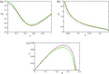
, in figure 1(a–c), respectively. Panel (a) indicates the transition from the stable region to the unstable one, through the change in the sign of product. The influence on the instability region is a decrease of the instability region (figure 1
a). It also shows how the threshold wavenumber
 $K_{c}$
changes with the non-extensive index
 $q$
(figure 1
b). The growth rate of the modulational instability was also investigated for different values of
 $q$
in panel (c). The growth rate is increased by the non-extensivity and thus the spectral index
 $q$
may be used as a controlling parameter for the modulational instability.
Variation of (a) the product
 $PQ$
, (b) the threshold wavenumber
 $K_{c}$
versus the carrier wavenumber
 $k$
and also (c) behaviour of the modulational instability growth rate
 $\unicode[STIX]{x1D6E4}$
versus the perturbation wavenumber
 $K$
for different values of the spectral index
 $q$
along with
 $q=1.1$
(solid curve),
 $q=1.2$
(dashed curve) and
 $q=1.5$
(dotted curve).

4 Localized solution of NLS equation
The occurrence of rogue waves (freak waves) associated with electromagnetic pulse propagation interacting with a plasma has been investigated by Veldes et al. (Reference Veldes, Borhanian, McKerr, Saxena, Frantzeskakis and Kourakis2013). They considered a set of non-stationary envelope solutions of the NLS equation (which governs the amplitude of the vector potential) as potential candidates for the modelling of rogue waves in beam–plasma interactions, in the form of the Peregrine soliton, the Akhmediev breather and the Kuznetsov–Ma breather. Going parallel to what has been done in Veldes et al. (Reference Veldes, Borhanian, McKerr, Saxena, Frantzeskakis and Kourakis2013), let us consider different localized solutions regarding analytical breather solutions of the NLS equation (3.9), and examine their properties in the frame of the present plasma system, i.e. a degenerate relativistic non-extensive plasma.
4.1 Peregrine’s soliton
The Peregrine paradigm (Peregrine Reference Peregrine1983; Dysthe & Trulsen Reference Dysthe and Trulsen1999; Shrira & Geogjaev Reference Shrira and Geogjaev2010) as a prototypical model for rogue waves has recently been employed successfully by Kibler et al. (Reference Kibler, Fatome, Finot, Millot, Dias, Genty, Akhmediev and Dudley2010) in nonlinear optics. Such a structure first appeared in the literature 30 years ago, and exhibits only a single rogue structure whose amplitude decreases in both time and space. The Peregrine solution has been examined experimentally in wave tank laboratories (Chabchoub, Hoffmann & Akhmediev Reference Chabchoub, Hoffmann and Akhmediev2011), in optical fibres (Kibler et al. Reference Kibler, Fatome, Finot, Millot, Dias, Genty, Akhmediev and Dudley2010) and also in plasma (Bailung, Sharma & Nakamura Reference Bailung, Sharma and Nakamura2011) situations. The analytical form of Peregrine’s soliton is given by
 $$\begin{eqnarray}\displaystyle \unicode[STIX]{x1D719}_{1}^{(1)}(\unicode[STIX]{x1D709},\unicode[STIX]{x1D70F})=\left[1-\frac{4+8\text{i}Q\unicode[STIX]{x1D70F}}{1+2Q\unicode[STIX]{x1D709}^{2}/P+4Q^{2}\unicode[STIX]{x1D70F}^{2}}\right]\text{e}^{\text{i}Q\unicode[STIX]{x1D70F}}, & & \displaystyle\end{eqnarray}$$
where
 $P$
and
 $Q$
refer to the coefficients of dispersive and nonlinear terms in (3.9), respectively. Recall that also the ‘slow’ variables
 $(\unicode[STIX]{x1D709},\unicode[STIX]{x1D70F})$
were defined in (3.2). This solution shows a non-trivial behaviour over a small region of
 $\unicode[STIX]{x1D709}$
and
 $\unicode[STIX]{x1D70F}$
, but it decays to a plane-wave asymptotic background for either large
 $\unicode[STIX]{x1D709}$
or
 $\unicode[STIX]{x1D70F}$
.
4.2 Akhmediev’s breather
The Akhmediev breather (Akhmediev, Eleonskii & Kulagin Reference Akhmediev, Eleonskii and Kulagin1987) as an exact solution of the NLS equation (3.9), describes the modulational instability in its nonlinear regime. The corresponding waveform shows a periodic structure in space but is localized in time, given by
 $$\begin{eqnarray}\displaystyle \unicode[STIX]{x1D719}_{1}^{(1)}(\unicode[STIX]{x1D709},\unicode[STIX]{x1D70F})=\left[1+\frac{(2-4a)\cosh (bQ\unicode[STIX]{x1D70F})+\text{i}b\sinh (bQ\unicode[STIX]{x1D70F})}{\sqrt{2a}\cos (w\sqrt{Q/2P}\unicode[STIX]{x1D709})-\cosh (bQ\unicode[STIX]{x1D70F})}\right]\text{e}^{\text{i}Q\unicode[STIX]{x1D70F}}, & & \displaystyle\end{eqnarray}$$
in which
 $w=2\sqrt{1-2a}$
,
 $b=2\sqrt{2a(1-2a)}$
and
 $a\in (0,1/2]$
are real parameters. The perturbation grows in the case of
 $1-2a>0$
, not surprisingly such behaviour corresponds to that obtained by performing a linear stability analysis of a Stokes wave solution of the NLS equation. The above solution (4.2) decays to a Peregrine solution in the limit of large enough spatial periods (Akhmediev et al.
Reference Akhmediev, Eleonskii and Kulagin1987). Indeed, for the large time limit the Akhmediev breather reduces to a plane wave plus a small perturbation. The absolute maximum of the solution (4.2), can be achieved after some straightforward manipulation, as
 $$\begin{eqnarray}\displaystyle \unicode[STIX]{x1D719}_{max}^{(A)}=1+2\sqrt{2a}. & & \displaystyle\end{eqnarray}$$
4.3 Kuznetsov–Ma breather
The Kuznetsov–Ma breather (Kuznetsov Reference Kuznetsov1977) as one of the breather solutions was originally proposed in by Kuznetsov (Reference Kuznetsov1977) and three years later by Ma (Reference Ma1979). Against the Akhmediev breather, for the large time limit the modulation for the Kuznetsov–Ma breather is never small (thus, it does not corresponds to the classical Benjamin–Feir instability). This waveform, in contrast to the Akhmediev breather, exhibits a periodic structure in time but is localized in space and is given by (Ma Reference Ma1979; Veldes et al. Reference Veldes, Borhanian, McKerr, Saxena, Frantzeskakis and Kourakis2013)
 $$\begin{eqnarray}\displaystyle \unicode[STIX]{x1D719}_{1}^{(1)}(\unicode[STIX]{x1D709},\unicode[STIX]{x1D70F})=\frac{\cos \left(\displaystyle \frac{s^{\prime }Q\unicode[STIX]{x1D70F}}{2}-2\text{i}\unicode[STIX]{x1D703}\right)-\cosh (\unicode[STIX]{x1D703})\cosh \left(s\sqrt{\displaystyle \frac{Q}{2P}}\unicode[STIX]{x1D709}\right)}{\cos \left(\displaystyle \frac{s^{\prime }Q\unicode[STIX]{x1D70F}}{2}\right)-\cosh (\unicode[STIX]{x1D703})\cosh \left(s\sqrt{\displaystyle \frac{Q}{2P}}\unicode[STIX]{x1D709}\right)}\text{e}^{\text{i}Q\unicode[STIX]{x1D70F}}, & & \displaystyle\end{eqnarray}$$
in which
 $s^{\prime }=2\sinh (2\unicode[STIX]{x1D703})$
,
 $s=2\sinh \unicode[STIX]{x1D703}$
and
 $\unicode[STIX]{x1D703}\in \text{Re}$
. Just like the Akhmediev breather, one can find the absolute maximum of the solution (4.4), which after some straightforward algebra leads to
 $$\begin{eqnarray}\displaystyle \unicode[STIX]{x1D719}_{max}^{(KM)}=1+2\cosh \unicode[STIX]{x1D703}. & & \displaystyle\end{eqnarray}$$
The analytical expressions (4.1), (4.2) and (4.4) show how the basic features (magnitude and periodicity) of rogue waves depend on the nonlinearity and dispersion coefficients. Recalling the functional dependence of
 $P$
and
 $Q$
on plasma parameters, this model allows one to investigate the parametric dependence on the spectral index
 $q$
. Next, we numerically analyse the breather structures (4.1), (4.2) and (4.4) to investigate the dependences of the formation and characteristics of such localized structures on the spectral index
 $q$
.
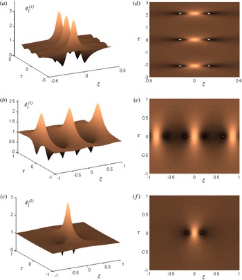
Figure 2 shows that the present plasma system supports excitation of localized structures with different periodicity characteristics in the time and space domains. According to (4.5), in figure 2(a), for
 $\unicode[STIX]{x1D703}=0.343$
we find that the maximum amplitude corresponds to
 $\unicode[STIX]{x1D719}_{max}^{(KM)}\cong 3.12$
. Also, for
 $a=0.25$
the maximum amplitude of the Akhmediev breather corresponds to
 $\unicode[STIX]{x1D719}_{max}^{(A)}\cong 2.41$
.
Profile of (a) Kuznetsov–Ma breather, (b) Akhmediev breather and (c) Peregrine soliton, and (d–f) their corresponding false colour plots, for
 $q=1.01$
and
 $k=1.5$
. In this case we have
 $Q=-4.05$
and
 $P=-0.074$
.

In order to investigate the effect of the spectral index
 $q$
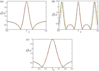
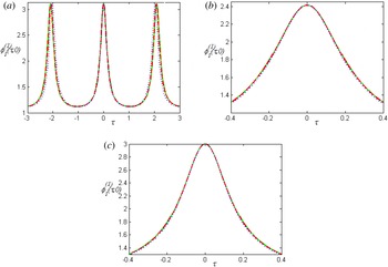
on the characteristic properties of such localized structures, we have considered a two-dimensional plot of
 $\unicode[STIX]{x1D719}_{1}^{(1)}(\unicode[STIX]{x1D709},\unicode[STIX]{x1D70F})$
in figure 3 (space extension) and figure 4 (time extension). As clearly shown in figure 3, the increase in spectral index
 $q$
decreases the extension of the excitation in the space domain in all three cases. On the other hand, an analogous trend occurs for the effect of
 $q$
on the time extension of the excitation structures (see figure 4). This is accompanied by increased time localization. It seems appropriate here to add that the breather solutions are related (Dysthe & Trulsen Reference Dysthe and Trulsen1999). It can be seen that the Akhmediev solution transfers to the Kuznetsov–Ma solution by replacing
 $\sqrt{Q/P}$
by
 $i\sqrt{Q/P}$
. On the other hand, in the limit of small values of
 $\sqrt{Q/P}$
(i.e.
 $\sqrt{Q/P}\rightarrow 0$
) the Akhmediev and the Kuznetsov–Ma solution reduce to the Peregrine solution. Also, for the large values of
 $\sqrt{Q/P}$
the Kuznetsov–Ma solution becomes a soliton, and for
 $a=1/2$
the Akhmediev solution reduces to the plane-wave solution.
The evolution of breather solutions of the NLS (3.11) with respect to the space coordinate
 $\unicode[STIX]{x1D709}$
, for the different values of the spectral index
 $q$
along with
 $q=1.1$
(solid curve),
 $q=1.2$
(dashed curve) and
 $q=1.5$
(dotted curve): (a) Kuznetsov–Ma breather, (b) Akhmediev breather and (c) Peregrine soliton. The parameters are:
 $k=1.5$
,
 $a=0.25$
and
 $\unicode[STIX]{x1D703}=0.343$
.

The evolution of breather solutions of the NLS (3.11) with respect to the time coordinate
 $\unicode[STIX]{x1D70F}$
, for the different values of the spectral index
 $q$
along with
 $q=1.1$
(solid curve),
 $q=1.2$
(dashed curve) and
 $q=1.5$
(dotted curve): (a) Kuznetsov–Ma breather, (b) Akhmediev breather and (c) Peregrine soliton. The parameters are:
 $k=1.5$
,
 $a=0.25$
and
 $\unicode[STIX]{x1D703}=0.343$
.

5 Conclusions
In the present study, the formation and characteristic properties of breather structures are studied in a non-extensive Thomas–Fermi plasma. Solving the fluid equations via a multiple scale technique, we have derived a NLS evolution for the amplitude of the electrostatic potential, describing the evolution of the localized structures. We have considered a set of breather-type solutions of NLS, and investigated the effect of non-extensive spectral index
 $q$
on their characteristics properties. The effect of spectral index
 $q$
on the dynamics has been examined by observing the influence of
 $q$
on (i) the stability/instability region (the wavenumber threshold dividing the carrier wavenumber domains into the stable and unstable regions), (ii) the growth rate of modulational instability and (iii) the localized profile characteristics (space–time localization). We find that the spectral index
 $q$
significantly affects the basic features of these localized excitations.
The influence on the instability region is a decrease of the instability region. The growth rate of the modulational instability was also investigated for different values of
 $q$
. The growth rate is increased by the non-extensivity and thus the spectral index
 $q$
may be used as a controlling parameter for the modulational instability.
The qualitative effect of electron non-extensivity on the localized excitation profile results in more space-extended as well as time-extended peak-shaped excitations.
The results of the present investigation must be useful to explain the basic features of nonlinear excitations associated with interstellar and space plasmas especially in stellar polytropes, protoneutron stars, hadronic matter and quark–gluon plasmas, dark-matter halos, etc. (Spruch Reference Spruch1991; Liolios Reference Liolios2003). It must be added that in the present numerical analysis, a wide range of degenerate plasma parameters was used, which are relevant for many compact astrophysical objects and cosmic environments, such as active galactic nuclei, the solar atmosphere, the primordial universe, pulsar magnetospheres, cores of giant planets such as Jupiter, neutron stars, supernovas, white dwarfs, etc. (Michel Reference Michel1982; Tandberg-Hansen & Emslie Reference Tandberg-Hansen and Emslie1988; Hoyos, Reisenegger & Valdivia Reference Hoyos, Reisenegger and Valdivia2008), hadronic matter and quark–gluon plasma (Gervino et al. Reference Gervino, Lavagno and Pigato2012), stellar polytropes (Plastino & Plastino Reference Plastino and Plastino1993), dark-matter halos (Feron & Hjorth Reference Feron and Hjorth2008), protoneutron stars (Lavagno & Pigato Reference Lavagno and Pigato2011) etc.
Appendix A
The coefficients of the harmonic modes in (3.6a )–(3.6c ) and (3.7a )–(3.7c ) are as follows
 $$\begin{eqnarray}\displaystyle \left.\begin{array}{@{}c@{}}\displaystyle A_{1}=[(c_{1}+k^{2})^{2}(2\unicode[STIX]{x1D714}kv_{g}+\unicode[STIX]{x1D714}^{2})-c_{2}k^{2}v_{g}^{2}]/(c_{1}v_{g}^{2}-1)k^{2},\\ \displaystyle A_{2}=[A_{1}k^{2}+(c_{1}+k^{2})^{2}(2\unicode[STIX]{x1D714}kv_{g}+\unicode[STIX]{x1D714}^{2})]/v_{g}^{2}k^{2},\quad \displaystyle A_{3}=A_{2}-2\unicode[STIX]{x1D714}(c_{1}+k^{2})/k,\\ \displaystyle A_{4}=\unicode[STIX]{x1D714}^{2}[3(c_{1}+k^{2})^{2}/2-c_{2}]/[c_{1}\unicode[STIX]{x1D714}^{2}+(4\unicode[STIX]{x1D714}^{2}-1)k^{2}],\\ \displaystyle A_{5}=[3(c_{1}+k^{2})^{2}/2-c_{2}]/3\unicode[STIX]{x1D714}^{2}+3(c_{1}+k^{2})^{2}/2,\\ \displaystyle A_{6}=\unicode[STIX]{x1D714}[3(c_{1}+k^{2})^{2}/2-c_{2}]/3k^{3}+\unicode[STIX]{x1D714}(c_{1}+k^{2})^{2}/2k.\end{array}\right\} & & \displaystyle\end{eqnarray}$$