








1 Introduction
Let
$\sigma _x(n) = \sum _{d \mid n} d^{x}$
 , and write
$\sigma _1(n) = \sigma (n)$
 . A perfect number is a positive integer n that satisfies
$\sigma (n) = 2n$
 . Similarly, a nondeficient number n is a positive integer that satisfies
$\sigma (n) \geq 2n$
 . The study of perfect numbers and of variants and generalizations of perfect numbers provides an active area within number theory. The purpose of this article is to disprove conjectures that were introduced by Ross in 2024 [Reference Ross12] and that concern nondeficient numbers and a variant of perfect numbers.
The study of perfect numbers has a long history, as discussed in the work of Ross [Reference Ross12] and the works cited therein, such as Hassler’s paper [Reference Hassler7] on the early history of perfect numbers. To this day, it is not even known whether or not there are infinitely many perfect numbers, and, indeed, this provides a well-known open problem in number theory. Similarly, it is currently not known whether or not there are any odd perfect numbers, and, again, this provides a well-known open problem in number theory. The foregoing considerations motivate the development of techniques in the study of perfect numbers and variants/generalizations of perfect numbers.
For an integer
$n> 1$
 , let the positive divisors of n be written so that

Let
$\mathcal {S}$
 be a set of integers. According to Ross [Reference Ross12], the integer n is said to be
$\mathcal {S}$
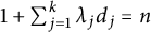
 -perfect if there are integers
$\lambda _1$
 ,
$\lambda _2$
 ,
$\ldots $
 ,
$\lambda _k \in \mathcal {S}$
 satisfying
$1 + \sum _{j=1}^{k} \lambda _j d_j = n$
 . Ross introduced and proved a characterization for all even
$\{ -1, 1 \}$
 -perfect numbers, and concluded with two conjectures that both concern both
$\{ -1, 1 \}$
 -perfect numbers and nondeficient numbers. Building on our extensive interactions with GPT-5.5 Pro, we disprove both of Ross’s conjectures.
1.1 Ross’s conjectures
A positive integer n is said to be abundant if
$\sigma (n)> 2 n$
 . Some authors, including Ross [Reference Ross12], use this same term to describe numbers n satisfying
$\sigma (n) \geq 2n$
 , as opposed to
$\sigma (n)> 2n$
 . For clarity, we make use of the standard definitions for abundant, nondeficient, and perfect numbers. We also restrict the notion of a number being
$\{ -1, 1 \}$
 -perfect to positive integers, as suggested above (and this agrees with the below conjectures from Ross).
As observed by Ross, every
$\{ -1, 1 \}$
 -perfect number is nondeficient, but it is not the case that every nondeficient number is
$\{ -1, 1 \}$
 -perfect [Reference Ross12]. This led Ross to conjecture that the
$\{ -1, 1 \}$
 -perfect numbers have a density equal to the density of the nondeficient numbers (cf. [Reference Ross12, Conjecture 16]). We disprove this conjecture in Section 2. This is motivated by the problem of evaluating the density of abundant numbers (reviewed in Section 1.2 below), and also by the recent work of Zelinsky on nondeficient numbers [Reference Zelinsky17].
Ross also observed that if an integer n is odd and nondeficient, then
$n^2$
 is also odd and nondeficient, but
$n^2$
 cannot be
$\{ -1, 1 \}$
 -perfect [Reference Ross12]. This led Ross to conjecture (see Conjecture 17) that every nonsquare odd nondeficient number is
$\{ -1, 1 \}$
 -perfect. We disprove this conjecture in Section 3.
1.2 Background
Since the first Ross conjecture given above in Section 1.1 concerns the natural density of nondeficient numbers, and since there has been much in the way of research related to the natural density of abundant numbers, we emphasize that these densities are equal. This follows from the density of perfect numbers being
$0$
 , which is well known, and which can be shown to follow from a result due to Davenport [Reference Davenport3] giving that the limit

exists and that the function of
$u \in [0, 1]$
 defined in (1.2) is continuous. A simplified proof of this result was subsequently given by Erdős [Reference Erdös5].
There have been many research efforts concerning the problem of estimating the density
$D\big ( \frac {1}{2} \big )$
 of abundant numbers. In this direction, a notable estimate is given by the bounds

given by Behrend in 1933 [Reference Behrend1]. Subsequent and notable refinements of (1.3) are due to Wall et al. [Reference Wall14–Reference Wall, Crews and Johnson16], Deléglise [Reference Deléglise4], and Kobayashi [Reference Kobayashi8]. Since the density of nondeficient numbers is
$D\big ( \frac {1}{2} \big )$
 , and again since the first Ross conjecture [Reference Ross12] reproduced in Section 1.1 concerns this same density, this motivates the techniques we apply in Section 2 to disprove the first Ross conjecture.
In addition to Ross’s definition of
$\mathcal {S}$
 -perfect numbers [Reference Ross12], many further extensions and variants of perfect numbers have been introduced and extensively studied. As indicated above, this forms a major area within number theory. In turn, this motivates our techniques applied in this article concerning the distributions of
$\{ -1, 1 \}$
 -perfect numbers and nondeficient numbers. Well-known extensions or variants of perfect numbers include sociable numbers (with the order-1 sociable numbers being perfect numbers), amicable numbers (which are order-2 sociable numbers), multiply perfect numbers, superperfect numbers, and hyperperfect numbers. Further examples of extensions/variants of perfect numbers include pseudoperfect numbers [Reference Sierpiński13], prime-perfect numbers [Reference Pollack and Pomerance10], s-near perfect numbers [Reference Pollack and Shevelev11], and within-perfect numbers [Reference Kwan and Miller9].
2 Disproof of Ross’s first conjecture
Following Ross [Reference Ross12], we write
$P(\mathcal {S})$
 for the set of positive
$\mathcal {S}$
 -perfect numbers, omitting the brackets associated with the notation for a given finite subset
$\mathcal {S}$
 of
$\mathbb {Z}$
 . We then let
$ \mathcal {P} = P(-1,1)$
 . Ross observed that the sequence of nondeficient numbers that are not
$\{ -1, 1 \}$
 -perfect begins with
$ 18$
 ,
$20$
 ,
$36$
 ,
$\ldots $
 Informally, our strategy to disprove Ross’s first conjecture may be thought of as being based on extending the first example of a nondeficient number that is not
$\{ -1, 1 \}$
 -perfect.
For a given set
$\mathcal {S}$
 of integers, we adopt the notational conventions such that

If the two values in (2.1) are equal, then we may write
$d(\mathcal S)$
 in place of their common value.
We write

The main goal of this section is to prove Theorem 2.4 below, giving us that there is a set
$ \mathcal {E} \subseteq \mathcal {A} \setminus \mathcal {P} $
 satisfying
$\underline d(\mathcal {E})>0$
 , that is, so that
$ \overline d(\mathcal {P})<d( \mathcal {A} ) $
 holds, thereby disproving Ross’s density conjecture [Reference Ross12, Conjecture 16] concerning
$\mathcal {P}$
 .
We begin with a reformulation, as below, of the definition of a
$\{ -1, 1 \}$
 -perfect number.
Lemma 2.1 For an integer n exceeding
$1$
 , let the positive divisors of n be written as in (1.1). Then,
$n \in \mathcal {P}$
 if and only if
$ \frac {\sigma (n)-2n}{2} $
 is a sum of distinct divisors chosen from
$d_1, d_2, \ldots ,d_k$
 , allowing for the possibility of an empty sum.
Proof Since
$ 1+\sum _{j=1}^k d_j = \sigma (n)-n$
 , by switching the sign of
$d_j$
 for a given index
$j \in \{ 1, 2, \ldots , k \}$
 , we see that: The existence of an expansion of the form
$ n=1+\sum _{j=1}^k c_jd_j $
 for
$c_j\in \{-1,1\}$
 is equivalent to the existence of a (possibly empty) subset
$T\subseteq \{1,\ldots ,k\}$
 such that
$ \sigma (n) - 2n = 2 \sum _{j \in T} d_j$
 , as desired.
Observe that Lemma 2.1 confirms that each positive
$\{-1,1\}$
 -perfect number is nondeficient (as observed by Ross [Reference Ross12]), since a (possibly empty) sum of divisors of the form given in Lemma 2.1 gives us that
$\sigma (n) - 2n \geq 0$
 .
We make use of standard notation for arithmetic functions, letting
$\omega (n)$
 denote the number of distinct prime factors of a positive integer n, letting
$\varphi (n)$
 denote the Euler totient function giving the number of integers
$m \in [1, n]$
 relatively prime with n, letting
$\pi (x)$
 denote the number of primes not exceeding x, and letting
$p_n\# = \prod _{i=1}^{n} p_{i}$
 denote the
$n^{\text {th}}$
 primorial. For an integer n exceeding
$1$
 , by writing
$n = \prod _{i=1}^{\omega (n)} p_{a_i}^{b_i}$
 , the relation

provides a basic property of the arithmetic function
$\sigma _x(n)$
 [Reference Hardy and Wright6, Section 16.7] and is required for our purposes.
We also require a standard consequence of Markov’s inequality, providing what may be seen as a “non-probabilistic” version of Markov’s inequality. Explicitly, if E is a finite set, then, for a function
$F\colon E \to [0, \infty )$
 and a positive value
$\eta $
 , we have that

Lemma 2.2 For every
$\varepsilon>0$
 , the set of positive integers m such that
$ (m,6)=1$
 and
$ \frac {\sigma (m)}{m}<1+\varepsilon $
 has positive lower asymptotic density.
Proof Let y be a real number such that
$y \geq 3$
 . We proceed to define

We rewrite the right-hand side of (2.5) as a union of residue classes modulo
$p_{\pi (y)}\#$
 , and we find that it has a natural density equal to

It is well known that the counting function for integers not exceeding
$x> 0$
 and coprime to a fixed modulus
$q \in \mathbb {Z}$
 is
$\frac {\varphi (q)}{q} x + O(1)$
 , with the error term
$O(1)$
 being uniform in x for every fixed q. Consequently, the relation

holds, with the error term in (2.7) being uniform in x (but dependent on y). Since
$y \geq 3$
 , we have that
$2 \mid p_{\pi (y)}\#$
 and
$3 \mid p_{\pi (y)}\#$
 . Consequently, the implication

holds. Now, we define

If
$m \in \mathcal {R}_{y}$
 , then each prime
$p \leq y$
 does not divide m. So, if
$m \in \mathcal {R}_{y}$
 , then, since each prime divisor of m is strictly greater than y, the right-hand side of (2.9) may be rewritten so that
$G_y(m) = \sum _{p \mid m} \frac {1}{p-1}$
 .
Now, by writing a positive integer m so that
$m = \prod _{p^b \Vert m} p^b$
 , this together with the relation in (2.3) give us that

If
$u \in (0, 1)$
 , then
$-\log (1-u) \leq \frac {u}{1-u}$
 . This together with the relation
$\log \frac {\sigma (m)}{m} \leq \sum _{p \mid m} - \log \left ( 1 - \frac {1}{p} \right )$
 give us that

So, from (2.10) along with how the right-hand side of (2.9) reduces for
$m \in \mathcal {R}_{y}$
 , we find that

By defining

we proceed to rewrite the right-hand side of (2.12) so that

Now, fix
$y \geq 3$
 . We rewrite the estimate in (2.7) so that

uniformly for real
$X> 0$
 , with the understanding that the error term in (2.14) depends only on y and not on X. Now, fix a prime
$p> y$
 . By writing
$m = p u$
 , we obtain that

with the understanding that u and m range over positive integers, and where, for the second-to-last equality above, we have exploited the property that
$p \nmid p_{\pi (y)}\#$
 , that is, since p does not divide the product of primes not exceeding
$y < p$
 . So, by setting
$X = \frac {x}{p}$
 in (2.14), this and the chain of five equalities above give us that

and we again emphasize that the error term in (2.15) depends only on y.
Now, from (2.13) and (2.15) together, we find that

From (2.16), we write

The convergence of
$\sum _{p} \frac {1}{p(p-1)}$
 together with the relation in (2.17) gives us that

Observe that
$ \sum _{p> y} \frac {1}{p(p-1)} \to 0$
 as
$y \to \infty $
 . So, for arbitrary
$\varepsilon> 0$
 , we may choose
$y = y_{\varepsilon } \geq 3$
 so that
$ \sum _{p> y} \frac {1}{p(p-1)} < \log (1 + \varepsilon )$
 .
Now, define

An application of the formulation of Markov’s inequality in (2.4) then gives us that

recalling (2.12). From (2.18) along with (2.20), we find that

Recalling the density of
$\mathcal {R}_{y}$
 shown in (2.7), we find that
$ \underline {d}\big ( \mathcal {R}_{y} \setminus \mathcal {B}_{y, \varepsilon } \big ) \geq \rho _y - \overline {d}(\mathcal {B}_{y, \varepsilon })$
 . Consequently, we obtain the relations

Now, if
$ m \in \mathcal {R}_{y} \setminus \mathcal {B}_{y, \varepsilon }$
 , then a combined application of the implication in (2.11) together with the complement of the right-hand side of (2.19) gives us that
$\log \frac {\sigma (m)}{m} \leq G_y(m) < \log (1 + \varepsilon )$
 , that is, so that

So, a combined application of the lower bound in (2.21) together with the implications in both (2.8) and (2.22) gives us that
$\mathcal {R}_{y} \setminus \mathcal {B}_{y, \varepsilon }$
 is a set of positive integers m that is of positive lower density such that both
$ (m,6)=1$
 and
$ \frac {\sigma (m)}{m}<1+\varepsilon $
 hold.
Lemma 2.3 Let m be a positive integer with
$(m,6)=1$
 , and put

If

then
$18m$
 is (strictly) abundant, but
$18m\notin \mathcal {P}$
 .
Proof We henceforth assume that (2.24) holds. Since m and
$6$
 are coprime, we find that
$(18, m) = 1$
 . Since
$\sigma $
 is multiplicative, we see that
$\sigma (18m) = 39 \sigma (m)$
 , so that (2.23) then gives us that
$\sigma (18m) = 39(m + s(m))$
 . Since
$m> 0$
 and
$s(m) \geq 0$
 , we find that
$\sigma (18m) - 2(18m) = 3 m + 39 s(m)> 0$
 . It follows that
$18m$
 is strictly abundant, in particular
$18 m \in \mathcal {A}$
 , and it remains only to be shown that also
$18 m \not \in \mathcal {P}$
 .
By way of contradiction, suppose that
$18 m \in \mathcal {P}$
 . So, by Lemma 2.1, the integer

can be written as a sum of distinct divisors of
$18m$
 apart from
$1$
 and
$18m$
 . We then rewrite (2.25) so that

With the assumption that (2.24) holds, we find that
$39 s(m) < \frac {m}{2}$
 . So, again with the assumption of (2.24) holding, we find that

Now, let
$\mathscr {S}$
 be a sum of proper (distinct) nontrivial divisors of
$18 m$
 . Since
$(18, m) = 1$
 , each divisor of
$18m$
 is of the form
$ed$
 for
$e \mid 18$
 and
$d \mid m$
 . We consider the two cases given by
$d = m$
 and
$d < m$
 . For the
$d = m$
 case, any such divisors appearing in the expansion of
$\mathscr {S}$
 as a sum of divisors of
$18 m$
 provide a contribution of
$A m $
 to
$\mathscr {S}$
 , for some integer
$A \geq 0$
 . We then write
$\mathscr {S} = A m + B$
 , where

Since
$\sum _{e \mid 18} e = \sigma (18) = 39$
 and since
$\sum _{\substack {d \mid m \\ d < m}} d = \sigma (m) - m = s(m)$
 , we find that
$0 \leq B \leq 39 s(m)$
 . So, the sum
$\mathscr {S}$
 is of the form
$ \mathscr {S} = A m + B $
 for a nonnegative integer A and for an integer
$B \in [0, 39s(m)]$
 . If
$A \leq 1$
 , then
$\mathscr {S} \leq m + 39 s(m)$
 , and from (2.24), we would then have that
$\mathscr {S} < \frac {3m}{2}$
 , so that
$\mathscr {S} < H$
 , recalling (2.26). Also, if
$2 \leq A$
 , then
$2m \leq \mathscr {S}$
 , but (2.26) gives us that
$H < 2m$
 , so that
$H < \mathscr {S}$
 . So, we have shown that no sum of proper, nontrivial divisors of
$18 m$
 can be equal to the right-hand side of (2.25), contradicting Lemma 2.1. Since we have shown that
$18 m \not \in \mathcal {P}$
 , we have completed our proof.
Theorem 2.4 There exists a set
$ \mathcal {E} \subseteq \mathcal {A} \setminus \mathcal {P} $
 satisfying
$\underline d(\mathcal {E})> 0$
 . Consequently, the strict inequality
$ \overline d(\mathcal {P})<d( \mathcal {A} ) $
 holds.
Proof By setting
$\varepsilon = \frac {1}{78}$
 in Lemma 2.2, we find that there exists a set
$\mathcal {M}$
 of positive integers such that

and such that: for each member m in
$\mathcal {M}$
 , we have that
$(m, 6) = 1$
 and that
$\frac {\sigma (m)}{m} < \frac {79}{78}$
 . Again for a member m of
$\mathcal {M}$
 , we set
$s(m) = \sigma (m) - m$
 . We then find that
$\frac {s(m)}{m} = \frac {\sigma (m)}{m} - 1 < \frac {1}{78}$
 . So, if
$m \in \mathcal {M}$
 , then m satisfies all of the required conditions in Lemma 2.3. So, if
$m \in \mathcal {M}$
 , then
$18 m$
 is strictly abundant and
$18 m \not \in \mathcal {P}$
 . Recalling the definition of
$\mathcal {A}$
 in (2.2), we thus find: if
$m \in \mathcal {M}$
 , then
$18m \in \mathcal {A} \setminus \mathcal {P}$
 . By then writing
$\mathcal {E}$
 in place of the family
$\{ 18 m : m \in \mathcal {M} \}$
 , we obtain the containment

Now, observe that

Taking lower limits with
$x \to \infty $
 , the relation in (2.29) then gives us that

So, from (2.27) and (2.30) together, we find that

Now, recall that every
$\{ -1, 1\}$
 -perfect number is a nondeficient number, as observed by Ross [Reference Ross12] (and recall that this also follows from Lemma 2.1). So, we find that the containment
$\mathcal {P} \subseteq \mathcal {A}$
 holds. From this containment together with the containment in (2.28), we find: for all
$x \geq 1$
 , the families
$\{ n \leq x : n \in \mathcal {P} \}$
 and
$\{ n \leq x : n \in \mathcal {E} \}$
 are disjoint and are both contained in the family
$\{ n \leq x : n \in \mathcal {A} \}$
 . Consequently, we obtain the relation

From (2.32), we find that

From (2.31) and (2.33) together, we have, as a consequence, that
$\overline {d}(\mathcal {P}) < d(\mathcal {A})$
 , as desired.
3 Disproof of Ross’s second conjecture
The following result gives an explicit family of counterexamples giving that Ross’s second conjecture [Reference Ross12, Conjecture 17] does not hold, by letting, for example,
$a = 945^2$
 , noting that
$945$
 is the smallest odd abundant number.
Theorem 3.1 Let a be an odd abundant square. If p is a prime such that
$p> \sigma (a)$
 , then
$n = a p$
 is an odd nonsquare abundant number, but
$n \not \in \mathcal {P}$
 .
Proof Let a denote an odd abundant square. Let p be a prime such that
$p> \sigma (a)$
 . We then write n in place of
$ap$
 . Since
$\sigma (a)> 2a$
 (from the assumption that a is strictly abundant), we find that
$p> \sigma (a) > 2a > a$
 , so that
$p \nmid a$
 . Moreover, since
$a \geq 1$
 , we have that
$p> 2$
 , so that n is odd. Since
$p \nmid a$
 , the exponent of p in the prime factorization of
$n = a p$
 is
$1$
 ; in particular, n is not a square.
Now, since
$(p, a) = 1$
 and since
$\sigma $
 is multiplicative, we find that
$\sigma (n) = \sigma (a) (p+1)$
 . As a consequence, we have that

It follows that n is abundant.
Since a is an odd square, we write

with
$a_i> 1$
 and
$c_i \geq 1$
 for all
$i \in \{ 1, 2, \ldots , \omega (a) \}$
 . From (2.3) and (3.2) together, we find that

with each factor on the right of (3.3) being odd, that is, so that
$\sigma (a)$
 is odd. So, the integer
$\Delta := \sigma (a) - 2 a$
 is odd. Also, with the assumption that a is abundant, we find that
$\Delta> 0$
 . So, there exists an integer
$q \geq 0$
 satisfying
$\Delta = 2 q + 1$
 . As a consequence of (3.1), we obtain that
$ \sigma (n) - 2 n = \Delta p + \sigma (a)$
 , and we define
$ H(n) := \frac {\sigma (n) - 2 n}{2}. $
 From this definition, we find that

Now, by way of contradiction, suppose that
$n \in \mathcal {P}$
 . So, by Lemma 2.1, the integer
$H(n)$
 can be written as a sum of proper (distinct) nontrivial divisors of n. Now, let
$\mathscr {S}$
 denote a sum of nontrivial and proper divisors of n. Since
$n = ap$
 and since a and p are relatively prime, each divisor of n is either a divisor d of a or is of the form
$dp$
 , again for a divisor d of a. This gives us that
$\mathscr {S} = A p + B$
 for some integer
$A \geq 0$
 and an integer B, which satisfies the bounds whereby
$0 \leq B \leq \sigma (a)$
 . From the condition
$\sigma (a) < p$
 , we find that

In a similar fashion, we have that

If
$A \leq q$
 , then
$Ap + B \leq q p + \sigma (a) < H(n)$
 , from (3.4). If
$A \geq q + 1$
 , then
$A p + B \geq (q+1) p> H(n)$
 , from (3.5). So, no divisor sum of the form
$\mathscr {S}$
 can be equal to
$H(n)$
 , contradicting (via Lemma 2.1) our assumption that
$n \in \mathcal {P}$
 .
So, we have shown that n is odd, nonsquare, and abundant, with
$n \not \in \mathcal {P}$
 .
4 Conclusion
As noted by an anonymous reviewer of this article, Theorem 2.4 suggests that the study of
$\{ -1, 1 \}$
 -perfect numbers is richer than Ross had envisioned [Reference Ross12], that is, since Theorem 2.4 can be thought of as formalizing how
$\{ -1, 1 \}$
 -perfect numbers are not “essentially the same as” nondeficient numbers. This motivates further research endeavors on
$\{ -1, 1 \}$
 -perfect numbers, along with further variants and extensions of the concept of a perfect number, as below.
An analog of perfect numbers defined using
$\sigma _a(n)$
 in place of
$\sigma (n)$
 was considered by Cai et al. in 2015 [Reference Cai, Chen and Zhang2]. Namely, Cai et al. considered an analog of perfect numbers given by natural numbers n such that

for fixed integer parameters
$a \geq 3$
 and
$b \geq 1$
 . This definition together with Ross’s definition of an
$\mathcal {S}$
 -perfect number motivate a common extension of both definitions, and we encourage the exploration of this.
One may also consider variants or analogs of perfect numbers defined via prime divisors. Since no natural number n satisfies
$\sum _{p \mid n} p = 2n$
 , and since n is prime if and only if
$\sum _{p \mid n} p = n$
 , it seems that prime divisor sum analogs of perfect numbers have not previously been considered. For a positive integer m, one may check that no natural number n satisfies
$\sum _{p \mid n} p = n + m$
 , which leads us to consider natural numbers n satisfying
$\sum _{p \mid n} p = n - m$
 , again for a fixed parameter
$m \in \mathbb {N}$
 . In turn, this leads us to define
$a(m)$
 as the number of positive integers n satisfying
$\sum _{p \mid n} p = n - m$
 , noting that it can be shown that
$a(m)$
 is always finite, using known properties of the sum-of-prime-divisors function. We encourage the investigation of the integer sequence
$(a(m) : m \in \mathbb {N})$
 and its number-theoretic properties. Are there infinitely many natural numbers m such that
$a(m) = 0$
 ? Is the sequence
$(a(m) : m \in \mathbb {N})$
 unbounded? What can be said in regard to growth properties of this sequence?
What we have referred to, as above, as
$\mathcal {S}$
 -perfect numbers are referred to as
$\mathcal {S}$
 -perfect numbers of the first kind by Ross [Reference Ross12]. What Ross referred to as
$\mathcal {S}$
 -perfect numbers of the second kind were briefly dealt with, and we encourage a full investigation of this latter family of extensions of perfect numbers. Omitting details, for brevity, it can be shown that both of Ross’s conjectures for
$\{ -1, 1 \}$
 -perfect numbers of the first kind are also false for
$\{ -1, 1 \}$
 -perfect numbers of the second kind, and (informally) this can be shown using the same constructions as above.
Observe that Theorem 2.4 gives us that either it is not the case that
$d(\mathcal {P})$
 exists or it is not the case that
$d(\mathcal {P}) = d(\mathcal {A})$
 . This raises a number of questions. What can be said in regard to whether or not the limit associated with
$d(\mathcal {P})$
 exists? How can suitable lower bounds be determined? We leave these questions for a future project.
Theorem 3.1 raises questions as to how odd
$\{ -1, 1 \}$
 -perfect numbers can be classified in full. This seems to be quite difficult, and we leave this as an open problem.
Acknowledgments
The author is very thankful for very detailed and exceptionally helpful referee feedback that has been provided and that has led to many improvements to this research paper. The quality of this research paper has been improved in a significant way because of the reviewer’s feedback that has been given. The author also thanks Joshua Zelinsky for some useful feedback, and the author acknowledges extensive interactions with GPT-5.5 Pro during the exploratory and proof-development stages of this work. All AI-generated suggestions were substantially revised, corrected, and independently verified by the author, who assumes full responsibility for the mathematical content.


