

1 Introduction
A homogeneous link is a link represented by a homogeneous diagram, a diagram whose Seifert graph is homogeneous. It is a common generalisation of alternating links and positive or negative links and has various nice properties.
Let
$\chi (L)$
 be the maximum Euler characteristic of Seifert surfaces of L and let
$P_L(v,z)$
 be the HOMFLY polynomial of a link L, given by the skein relation

In [Reference Cromwell4, Theorem 4(b)], Cromwell proved the following result which we call the Cromwell inequality.
Theorem 1.1 (Cromwell inequality)
For a homogeneous link L,

Furthermore, (1.1) is an equality if and only if L is positive.
In [Reference Cromwell4], the link is always assumed to be nonsplit and the theorem is proved for nonsplit links, but one can check that the theorem also applies for split links.
For a link L with homogeneous diagram D, Seifert’s algorithm gives a maximum Euler characteristic Seifert surface of L; hence,
$\chi (L)=s(D)-c(D)$
 , where
$s(D)$
 is the number of Seifert circles and
$c(D)$
 is the number of crossings of D [Reference Cromwell4, Corollary 4.1]. Thus, we may understand Theorem 1.1 as the inequality

for a homogeneous diagram D of L.
The aim of this note is to give a strengthened version of Cromwell’s inequality. We point out that Cromwell’s argument, as we will state in Theorem 2.2, actually proves a much stronger result than stated in Theorem 1.1. Based on this observation, we prove the following generalisation of the diagram version of the Cromwell inequality (1.2).
Theorem 1.2. For a homogeneous link L with homogeneous diagram D,

Here,
$w(D)$
 is the writhe of D,
$s_+(D)$
 is the number of connected components of the diagram obtained from D by resolving all the negative crossings of D and
$\#_{\mathrm {sp}} L$
 is the number of split components of L.
The right-hand side in Theorem 1.2 appears in the following so-called sharper Bennequin-type inequality. Let
$\chi _4(L)$
 be the maximum Euler characteristic of a smoothly embedded surface in
$B^{4}$
 whose boundary is L. A slice-torus invariant of a knot is a homomorphism
$\phi :\mathcal {C} \rightarrow \mathbb {R}$
 from the smooth knot concordance group
$\mathcal {C}$
 to
$\mathbb {R}$
 , such that
$\phi (T_{p,q})= g_4(T_{p,q})$
 for the
$(p,q)$
 -torus knot
$T_{p,q}$
 [Reference Lewark7]. For the definition of the slice-torus invariant of links, we refer to [Reference Cavallo and Collari2].
Theorem 1.3 [Reference Cavallo and Collari2, Theorem 1.4]
Let
$\phi $
 be a slice-torus invariant. Then, for a link L and its nonsplittable diagram D,

Here,
$\#L$
 denotes the number of components of L, and a nonsplittable diagram D is one for which the number of connected components of D is equal to
$\#_{\mathrm {sp}} L$
 , the number of split components of L.
Since a homogeneous diagram is nonsplittable [Reference Cromwell4, Corollary 3], Theorems 1.2 and 1.3 upgrade the Cromwell inequality (1.1) to the slice Cromwell inequality.
Corollary 1.4 (Slice Cromwell inequality)
For a homogeneous link L,

Remark that
$\min \deg _{v} P_L(v,z)$
 appears in the Morton–Franks–Williams inequality [Reference Franks and Williams5, Reference Morton8]

for the maximum self-linking number

Theorem 1.2 says that for homogeneous links, the Morton–Franks–Williams inequality subsumes all the Bennequin-type inequalities

of the slice-torus invariants
$\phi $
 .
As a generalisation of the condition for equality in the Cromwell inequality, we pose the following conjectures.
Conjecture 1.5. Let L be a homogeneous link.
-
(i) The slice Cromwell inequality is an equality if and only if L is positive.
-
(ii) For a homogeneous diagram D of L, the inequality in Theorem 1.2 is an equality if and only if D is a positive diagram.
Conjecture 1.5 is related to the following problem asked by Baader [Reference Baader1].
Question 1.6. Is a homogeneous quasipositive link positive?
Here, a link L is called quasipositive if it is a closure of a quasipositive braid, a product of conjugates of the positive generators
$\sigma _{1},\ldots ,\sigma _{n-1}$
 of the braid group.
Although Question 1.6 remains open even for alternating links, in [Reference Ito6], extending the argument in the alternating link case [Reference Orevkov10], we gave a partial affirmative answer. We showed that if a homogeneous link L admits a homogeneous diagram that attains the maximum self-linking number (for example, when the number of Seifert circles of D is equal to the braid index of L), then L is quasipositive if and only if the diagram is positive.
Conjecture 1.5 leads to an affirmative answer to Question 1.6.
Theorem 1.7. If Conjecture 1.5(i) or (ii) is true, quasipositive homogeneous links are positive.
Proof. For a homogeneous link L with homogeneous diagram D,

Since
$-\chi _4(L)=\overline {sl}(L)$
 holds for a quasipositive link L [Reference Rudolph11], it follows that a quasipositive homogeneous link attains the equality for both the slice Cromwell inequality and Theorem 1.2. Thus, assuming Conjecture 1.5(i) or (ii), we conclude that L is positive.
Finally, we point out that Theorem 2.2, which contains the actual content of Cromwell’s proof, can be used to solve [Reference Ohtsuki9, Problem 1.16] and [Reference Stoimenow13, Conjecture 4.1] concerning the signature
$\sigma (L)$
 and the minimum degree of the HOMFLY polynomial for alternating links.
We remark that [Reference Ohtsuki9, Problem 1.16] and [Reference Stoimenow13, Conjecture 4.1] also ask for the inequality
$\min \deg _a F_L(a^{-1},z) \leq \min \deg _v P_L(v,z)$
 for the Kauffman polynomial
$F_L(a,z)$
 , but this inequality was already proven in [Reference Rutherford12, Corollary 5.4]. Also, we remark that for the signature
$\sigma $
 , we are using the convention that
$\sigma (\mbox {Positive trefoil})=2$
 .
Theorem 1.8. For an alternating link L,

The anonymous referee pointed out that Theorem 1.8 also follows from Theorems 1.2, 1.3 and the equality
$\sigma (L)=2\phi (L)-\#L +1$
 for a nonsplit alternating link L and a slice-torus invariant
$\phi $
 [Reference Cavallo, Collari and Conway3, (2.10)]. (Note the different convention on the signature
$\sigma $
 in [Reference Cavallo, Collari and Conway3].)
2 Proof of Theorem 1.2
Let G be a signed graph which is not necessarily connected, but is not allowed to have a self-loop. A signed graph means that the sign
$+$
 or
$-$
 is assigned to each edge. A signed graph is positive (respectively negative) if all the signs of the edges are positive (respectively negative).
A vertex v of a graph G is a cut vertex if removing v increases the number of connected components. By splitting the graph along its cut vertices, each graph is decomposed as a union of blocks, connected maximum subgraphs without cut vertices. The rank of a graph G is defined by
$\operatorname {\mathrm {rank}}(G)= -\#V(G)+\#E(G)+\#G$
 , where
$V(G)$
 and
$E(G)$
 denote the set of vertices and edges of G, and
$\#G$
 denotes the number of connected components of G.
The Seifert graph
$G_D$
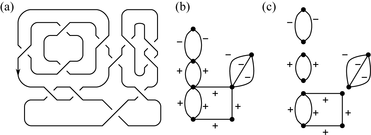
 of a link diagram D is a signed graph whose vertices are Seifert circles and whose edges are crossings (see Figure 1).
Definition 2.1 (Homogeneous graphs and links)
A signed graph is homogeneous if each block is either positive or negative. A link diagram D is homogeneous if its Seifert graph
$G_D$
 is homogeneous.
(a) Homogeneous diagram; (b) Seifert graph; (c) the blocks of the Seifert graph.

Figure 1 Long description
Panel a shows a complex homogeneous knot diagram consisting of multiple interlocking loops and crossings. The diagram features a large central rectangular loop surrounded by smaller nested and adjacent loops with alternating over-under crossings. An arrow on the left side indicates the orientation of the knot.
Panel b displays the Seifert graph derived from the knot. It consists of black nodes connected by curved and straight edges. The graph is structured with a vertical stack of three oval-shaped cells on the left and a square-like cell on the right. Edges are labeled with plus or minus signs to indicate crossing types. The vertical stack has signs minus, plus, plus from top to bottom. The right-hand structure includes a triangular loop with two internal minus signs and a square base with plus signs.
Panel c illustrates the blocks of the Seifert graph separated into four distinct components.
- The top component is a single oval with two minus signs.
- Below it is another oval with two plus signs.
- To the right is a triangular block containing two minus signs.
- At the bottom is a larger rectangular block with an oval on its left side, all labeled with plus signs.
To prove Theorem 1.2, we pin down what Cromwell actually proved in his proof of the Cromwell inequality.
Theorem 2.2 (Cromwell [Reference Cromwell4])
Let D be a connected homogeneous diagram of a link L. Let
$B_{i}\ (i=1,\ldots ,d)$
 be the blocks of its Seifert graph
$G_D$
 . Then,
$P_{L}(v,z)$
 contains a monomial
$v^{a}z^{b}$
 with
$a=\sum _{i=1}^{d}\varepsilon (B_i)\operatorname {\mathrm {rank}}(B_i)$
 and
$b=\operatorname {\mathrm {rank}} G_D\ (= 1-\chi (L))$
 . Here,
$\varepsilon (B_i)$
 is the sign of the block
$B_i$
 .
For the reader’s convenience, we give a brief outline of the proof, emphasising the key properties derived from the proof.
Sketch of proof of Theorem 2.2
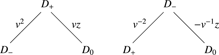
Starting from a given diagram D of a link L, the HOMFLY polynomial can be computed by applying the skein relation repeatedly. Such a computation is summarised by a so-called skein (resolution) tree, a rooted binary tree having the following properties.
-
• Each node is labelled by a link diagram and each edge is labelled by a monomial.
-
• The root is labelled by the diagram D.
-
• The triple $(D_{\mathrm {parent}},D_{\mathrm {child 1}},D_{\mathrm {child 2}})$
 consisting of the diagram
$D_{\mathrm {parent}}$
associated to a nonterminal node and the diagrams
$D_{\mathrm {child 1}},D_{\mathrm {child 2}}$
associated to its child nodes forms a skein triple
$(D_+,D_-,D_0)$
or
$(D_{-},D_+,D_0)$
. In the former case, the edge connecting
$D_{\mathrm {parent}}$
to
$D_{\mathrm {child 1}}$
(respectively
$D_{\mathrm {parent}}$
to
$D_{\mathrm { child 2}}$
) is labelled by the monomial
$v^{2}$
(respectively
$vz$
). In the latter case, the edge connecting
$D_{\mathrm {parent}}$
to
$D_{\mathrm {child 1}}$
(respectively
$D_{\mathrm {parent}}$
to
$D_{\mathrm {child 2}}$
) is labelled by the monomial
$v^{-2}$
(respectively
$-v^{-1}z$
) (see Figure 2).
Figure 2
Skein resolution tree.
-
• A diagram associated with a terminal node represents the unlink.


By the skein relation of the HOMFLY polynomial, the HOMFLY polynomial
$P_L(v,z)$
 is given by

where the summation runs over all the terminal nodes n,
$\pi (n)$
 is the product of labels of edges that appear in the path from the terminal node n to the root, and
$\#n$
 is the number of components of the unlink associated to the terminal node n.
Cromwell showed that in an appropriate skein tree coming from an ascending diagram construction, if a terminal node n satisfies
$\max \deg _z \pi (n) ({(v^{-1}-v)}/{z})^{\#n-1} = \operatorname {\mathrm {rank}} G_D$
 (that is, if a terminal node n contributes the highest z-degree terms of
$P_L(v,z)$
 ), it has the following properties.
-
(a) The Seifert graph of a diagram associated to n is a tree. Hence, it represents the unknot and $\pi (n) ({(v^{-1}-v)}/{z})^{\#n-1} = \pi (n)$
is a monomial. -
(b) The sign of the monomial $\pi (n) ({(v^{-1}-v)}/{z})^{\#n-1}$
does not depend on the choice of such a terminal node n. The sign is given by
$\prod _{i=1}^{d} \varepsilon (B_i)^{\operatorname {\mathrm {rank}} B_i}$
. In particular, contributions of the terminal nodes never cancel.


Then, the assertion comes from an observation that for the terminal node
$n_0$
 obtained by repeatedly resolving the crossings (that is, the rightmost terminal node), its contribution is given by

We rewrite
$\sum _{i=1}^{d}\varepsilon (B_i)\operatorname {\mathrm {rank}}(B_i)$
 in terms of the quantities from the diagram, rather than its Seifert graph.
Proposition 2.3. For a connected homogeneous diagram D,

Proof. Let P and N be the number of positive and negative blocks, and let
$B^{+}_1,\ldots , B^{+}_P$
 (respectively
$B^{-}_1,\ldots , B^{-}_N$
 ) be the positive (respectively negative) blocks of
$G_D$
 .
In the procedure for the decomposition of the Seifert graph
$G_D$
 into its blocks, cutting a graph at a cut vertex increases the number of vertices by one. Therefore,

Similarly,
$s_+(D)$
 is the number of connected components of the graph obtained by deleting all the negative-signed edges, Hence,

Thus,

Next, we prove the following assertion which is a bit stronger than Theorem 1.2.
Theorem 2.4. For a homogeneous link L with homogeneous diagram D, let
$h_L(v) \in \mathbb {Z}[v,v^{-1}]$
 be the highest z-degree term of the HOMFLY polynomial
$P_L(v,z)$
 of L, the coefficient of
$z^{1-\chi (L)}$
 . Then,
$h_L(v)$
 contains a monomial
$v^{-s(D)+w(D)+2s_+(D)+1-2\#_{\mathrm {sp}} L}$
 . In particular,

Proof. The case for L nonsplit follows from Theorem 2.2 and Proposition 2.3.
For a split link
$L=L_1 \sqcup L_2 \sqcup \cdots \sqcup L_{\#_{sp} L}$
 , its homogeneous diagram D is a disjoint union of the homogeneous diagrams
$D_i$
 of
$L_i$
 . Hence,

Remark 2.5. The inequality

in Theorem 2.4 often attains the equality for nonpositive diagrams, even for alternating links. For example, a nonpositive alternating knot
$6_1$
 attains the equality. Thus, we cannot prove Conjecture 1.5(i) and (ii) just by looking at the highest z-degree part
$h_L(v)$
 of the HOMFLY polynomial.
The proof of Theorem 1.8 is similar to the proof of Theorem 1.2. We observe that
$\sum _{i=1}^{d}\varepsilon (B_i)\operatorname {\mathrm {rank}}(B_i)$
 is nothing but the signature for alternating diagrams.
Proof of Theorem 1.8
For a connected, reduced alternating diagram D of a link L, the signature is given by

where
$d_{\pm }$
 is the number of positive and negative edges of a spanning tree of the Seifert graph
$G_D$
 [Reference Traczyk14, Theorem 2(1)]. Let
$B^{+}_1,\ldots , B^{+}_P$
 (respectively
$B^{-}_1,\ldots , B^{-}_N$
 ) be the positive (respectively negative) blocks of the Seifert graph
$G_D$
 . We remark that the formula in [Reference Traczyk14, Theorem 2(1)] contains an erroneous factor
$\tfrac 12$
 .
Since
$d_+ = \sum _{i=1}^{P}(\#V(B_i^+) -1)$
 and
$d_{-} = \sum _{i=1}^{N}(\#V(B_i^-) -1) $
 , we conclude

By Theorem 2.2, this shows the theorem for the nonsplit case. The split case follows easily from the nonsplit case.
Acknowledgement
The author gratefully thanks the anonymous referee for the alternative proof of Theorem 1.8.