1. Introduction
The Rayleigh–Taylor instability (Rayleigh Reference Rayleigh1883; Taylor Reference Taylor1950) has received sustained research interest over the past century. Many natural occurrences of the flow have been discovered and the uses and applications of the instability have been increasingly exploited (see Zhou (Reference Zhou2017a,Reference Zhoub) for a comprehensive recent review of the subject, or for example Boffetta & Mazzino (Reference Boffetta and Mazzino2017)). The original work of Rayleigh considered the instability due to heavier fluid overlaying lighter fluid in both cases of either a continuous or a step density stratification. In 1950 Taylor showed that the instability due to a heavy uniform layer overlying a light uniform layer under the action of gravity was identical to that of a stable two-layer stratification being accelerated vertically downwards at a rate greater than gravity. The initial linear growth rate is determined by the wavelength of a given perturbation, the effective gravitational acceleration that the system experiences and the density contrast between the two fluids. The growth rate may be further affected by fluid viscosity and surface tension between the fluid layers. To some extent these fluid properties are set by the situation in which the instability is occurring and there may not be a way for these properties to be manipulated if the intention is to influence the instability in some beneficial way. As such, investigators have sought to understand the influence of long-range effects, including rotation and magnetic fields on the instability (see e.g. Chandrasekhar Reference Chandrasekhar1961). A further motivation for such study is that the presence of strong rotation and magnetic fields in astrophysical scale flows is commonly understood to occur. Previous studies have considered rotation perpendicular or parallel to a density stratification (e.g. Dávalos-Orozco Reference Dávalos-Orozco1993; Carnevale et al. Reference Carnevale, Orlandi, Zhou and Kloosterziel2002; Tao et al. Reference Tao, He, Ye and Busse2013) or more general rotation of the system (e.g. Dávalos-Orozco & Aguilar-Rosas Reference Dávalos-Orozco and Aguilar-Rosas1989a,Reference Dávalos-Orozco and Aguilar-Rosasb; Dávalos-Orozco Reference Dávalos-Orozco1996a,Reference Dávalos-Orozcob). As these studies have been often motivated by astrophysical applications (e.g. García-Senz, Cabezon & Domínguez Reference García-Senz, Cabezon and Domínguez2018) the influence of viscosity on the development of the instability has not necessarily been considered, though investigations have been conducted into the global stability of rotating viscous systems (e.g. Joseph et al. Reference Joseph, Renardy, Renardy and Nguyen1985). Here our emphasis is on the effects of viscosity on the growth rate of the three-dimensional rotating Rayleigh–Taylor instability in a cylindrical domain with an initially cylindrical interface between the two fluids that may support surface tension effects.
Recent work has considered the effect of rotation on the Rayleigh–Taylor instability both experimentally (Baldwin, Scase & Hill Reference Baldwin, Scase and Hill2015; Scase, Baldwin & Hill Reference Scase, Baldwin and Hill2017a, Reference Scase, Baldwin and Hill2020) and theoretically (Scase, Baldwin & Hill Reference Scase, Baldwin and Hill2017b) in the low rotation rate limit focussing on the importance of the initial hydrostatic state. This work builds upon previous studies by Chandrasekhar (Reference Chandrasekhar1961) and Miles (Reference Miles1964). Chandrasekhar considered the effect of rotation on a two-layer unstable stratification with an initially planar interface. However, Miles showed that the frequency of free-surface oscillations predicted by Lamb (Reference Lamb1932) on a body of rotating liquid were in error, due to the assumption of a planar free-surface, by the same order of magnitude as the correction for rotation. In Scase & Hill (Reference Scase and Hill2018) the authors consider the high rotation limit of the Rayleigh–Taylor instability in inviscid and viscous configurations and investigate the effects of surface tension and interfacial diffusion. However, this study was strictly two-dimensional, considering only azimuthal perturbations to two fluid layers confined in a circular domain; the effect of axial perturbations was necessarily neglected. Here we extend that study to three dimensions.
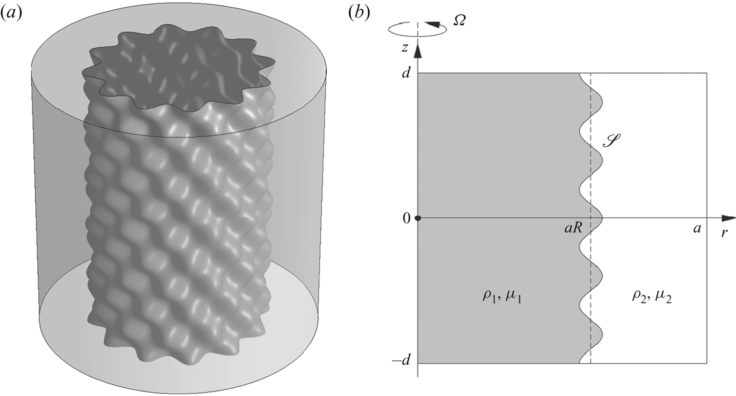
We consider an inner cylindrical column of fluid surrounded by an outer fluid layer all within a cylindrical container (unlike Weidman, Goto & Fridberg (Reference Weidman, Goto and Fridberg1997) and Dávalos-Orozco & Vázquez-Luis (Reference Dávalos-Orozco and Vázquez-Luis2003), we do not consider the case of a solid inner cylinder such as in a Taylor–Couette configuration). The outer fluid may differ from the inner fluid both in density and viscosity. The fluids are considered initially to be ‘spun-up’ into solid-body rotation (there is no initial shear between the fluid layers unlike one of the cases considered by Hocking & Michael (Reference Hocking and Michael1959)). We further allow for the possibility that there may also be surface tension between the two fluid layers. We consider the system as the extreme high rotation rate limit of the rotating Rayleigh–Taylor instability, where the influence of gravity may be neglected; it may be considered as a fully three-dimensional fluid–fluid centrifuge for cases where a Hele-Shaw approximation is not appropriate. The set-up is illustrated in figure 1 for an axial wavenumber  $n = 10$ and azimuthal wavenumber
 $m = 12$. By considering the system in the limits of high and low viscosity we are able to show the dependence of the growth rate on the Ekman number,
 $Ek$, that characterises the relative importance of viscosity to rotation. When the system is in the low viscosity regime,
 $Ek\ll 1$, the effect of viscosity is to modify the inviscid growth rate by an order
 $Ek^{1/2}$ correction that we derive. Conversely, when the system is in the high viscosity regime,
 $Ek\gg 1$, the instability growth rate behaves as
 $Ek^{-1}$. The effect of surface tension in the unstable configuration is to suppress the growth rate and possibly completely stabilise otherwise unstable modes of instability. The effect is greatest upon perturbations with the shortest wavelengths.
(a) The initial perturbation for axial wavenumber  $n = 10$ and azimuthal wavenumber
 $m = 12$. If the inner fluid layer is denser than the outer the perturbation on the interface will grow as the two fluids move in opposite radial directions. (b) Schematic of the meridional plane. Quantities associated with the inner layer have subscript 1, quantities associated with the outer layer have subscript 2. The interface,
 $\mathscr {S}$, is a perturbation about
 $r = aR$ (using dimensional quantities).

A special case of the flow configuration investigated is that of a rotating viscous column of fluid. In § 4 we examine this limit by allowing the density and viscosity of the outer fluid layer to tend to zero. Important applications of this flow are discussed in Kubitschek & Weidman (Reference Kubitschek and Weidman2007a) together with a linear stability analysis. As part of their extensive study, Kubitschek & Weidman (Reference Kubitschek and Weidman2007a) considered which mode of instability has the greatest growth rate in the limit of high viscosity and high surface tension. They established that in this region the two most unstable modes are an axisymmetric ‘varicose’ mode and a ‘spiral’ mode. Their numerical results suggested that there is an asymptotic form of the boundary at which the preferred mode of instability switches from varicose to spiral. We are able to derive and confirm their conjectured form of this boundary.
Though our flow configuration is idealised, it provides a connection between practical, realisable flows including, amongst others, stable coating flows on the inside of cylinders (e.g. Johnson Reference Johnson1988) with applications in turbojet engine cooling (e.g. Chew Reference Chew1996), unstable liquid atomisation and combustion flows (discussed in Kubitschek & Weidman (Reference Kubitschek and Weidman2007a)) and liquid jet instability in fusion processes (e.g. Chen, Schrock & Peterson Reference Chen, Schrock and Peterson1997).
The layout of the paper is as follows. In § 2 we introduce the governing model and the required boundary conditions and matching conditions at the interface between the two fluids. We first find a dispersion relation for the development of the instability for two inviscid fluid layers that may have surface tension acting between them. We then develop the inviscid solution by considering an asymptotic correction for the case of weakly viscous fluid layers. We next consider the case of highly viscous fluid layers and derive an expression for the growth rate in the case of equal viscosity in each layer (the full solution for highly viscous fluids with a viscous contrast is given in appendix B). In § 3 we show the results of numerical simulations of the instability in both high and low viscosity cases and compare the observed growth rates of the simulations with the theoretical predictions of § 2 and show that they are in good agreement. In § 4 we investigate the special limiting case of a rotating viscous column. Finally, in § 5 we draw our conclusions.
2. Modelling
We consider two layers of uniform density and uniform viscosity fluid arranged as concentric cylinders. The equations of motion for the fluid velocity  $\boldsymbol {u}_i$ and pressure
 $p_i$, in each layer
 $i=1$ (inner) and
 $i=2$ (outer) are the rotating Navier–Stokes equations with incompressibility given by
 \begin{gather} \rho_i \frac{\textrm{D} \boldsymbol{u}_i}{\textrm{D} t} = -\boldsymbol{\nabla} p_i - \rho_i \boldsymbol{\varOmega}\times\left(\boldsymbol{\varOmega}\times\boldsymbol{x}\right) - 2\rho_i \boldsymbol{\varOmega}\times\boldsymbol{u}_i + \mu_i\nabla^2\boldsymbol{u}_i, \end{gather}
 \begin{gather}\boldsymbol{\nabla}\boldsymbol{\cdot}\boldsymbol{u}_i=0. \end{gather}
We work in cylindrical polar coordinates with unit basis vectors  $\hat {\boldsymbol {r}}$,
 $\hat {\boldsymbol {\theta }}$ and
 $\hat {\boldsymbol {z}}$ in the radial, azimuthal and axial directions, respectively. Here
 $\boldsymbol {\varOmega }$ is the rotation vector, taken without loss of generality to be
 $\boldsymbol {\varOmega } = \varOmega \,\hat {\boldsymbol {z}}$. Following Scase & Hill (Reference Scase and Hill2018) we non-dimensionalise time by
 $\varOmega ^{-1}$, and length by the radial extent of the domain
 $a$ (see figure 1). The density and viscosity in each layer is non-dimensionalised as in Scase & Hill (Reference Scase and Hill2018) using a system mean density
 $\rho _0 = (\rho _1 + \rho _2)/2$ and system mean viscosity
 $\mu _0 = (\mu _1 + \mu _2)/2$. Hence we have that
 \begin{gather} \frac{\textrm{D} \boldsymbol{u}_i}{\textrm{D} t} = -\frac{1}{\rho_i}\boldsymbol{\nabla} p_i + r\,\hat{\boldsymbol{r}} - 2\hat{\boldsymbol{z}}\times\boldsymbol{u}_i + Ek\frac{\mu_i}{\rho_i}\nabla^2\boldsymbol{u}_i, \end{gather}
 \begin{gather}\boldsymbol{\nabla}\boldsymbol{\cdot}\boldsymbol{u}_i=0, \end{gather}
where all quantities are non-dimensional and the Ekman number characterizing the relative importance of viscosity to rotation is defined by  $Ek =\mu _0/\rho _0\varOmega a^2$. The non-dimensional density
 $\rho _i\in [0, 2]$ and the non-dimensional viscosity
 $\mu _i\in [0, 2]$. We now proceed by defining the linear differential operator,
 $\mathcal {L}$, by
 \begin{equation} \mathcal{L}[\phi] = \left(\frac{1}{2}\frac{\partial}{\partial t} - \frac{Ek}{2}\frac{\mu_i}{\rho_i}\nabla^2\right)\phi. \end{equation}
We are able to write the velocity and pressure perturbations to the hydrostatic initial condition in terms of a generalised potential,  $\phi$, in each layer (Hart Reference Hart1981) as
 \begin{gather} \boldsymbol{u}_i = \epsilon\left\{\left(1 + \mathcal{L}^2\right)\boldsymbol{\nabla}\phi_i - \mathcal{L}\left[\hat{\boldsymbol{z}}\times\boldsymbol{\nabla}\phi_i\right] + \hat{\boldsymbol{z}}\times\left(\hat{\boldsymbol{z}}\times\boldsymbol{\nabla}\phi_i\right)\right\}, \end{gather}
 \begin{gather}p_i = p_{0i}(\boldsymbol{x}, t) - 2\epsilon\rho_i\left(1 + \mathcal{L}^2\right)\mathcal{L}[\phi_i], \end{gather}
where  $|\epsilon |\ll 1$. For suitable
 $p_{0i}$ in each layer, this posed ansatz satisfies the equation of motion (2.2a) at leading order and at order
 $\epsilon$. The incompressibility condition (2.2b) leads to the governing equation for the generalised potential. Noting that
 $\boldsymbol {\nabla }\boldsymbol {\cdot }(\hat {\boldsymbol {z}}\times \boldsymbol {\nabla }\phi _i)\equiv 0$ and that
 $\boldsymbol {\nabla }\boldsymbol {\cdot }[\hat {\boldsymbol {z}}\times (\hat {\boldsymbol {z}}\times \boldsymbol {\nabla }\phi _i)] = -\nabla ^2_H\phi _i$, where we define the horizontal Laplacian
 $\nabla ^2_H = \partial _{rr} + r^{-1}\partial _r + r^{-2}\partial _{\theta \theta }$, we have that
 \begin{equation} \left(1 + \mathcal{L}^2\right)\nabla^2\phi_i - \nabla^2_H\phi_i=0, \end{equation}
a sixth-order, linear partial differential equation for  $\phi _i$.
The initial unperturbed location of the interface is taken to be at  $r=R$ for
 $R\in (0,1]$ (see figure 1) and we assume that the position of the perturbed interface between the two fluid layers is given by
 $\mathscr {S}$ where
 \begin{equation} \mathscr{S} := r - \left( R + \epsilon \cos\left(\frac{n{\rm \pi} \left[z - \delta\right]}{2\delta}\right)\exp({\textrm{i}\left(m\theta + \omega t\right)})\right) = 0, \end{equation}
for axial (varicose) wavenumber  $n\in \mathbb {N}$, azimuthal wavenumber
 $m\in \mathbb {N}$ and domain aspect ratio
 $\delta = d/a$, and note that this definition of the interface sets the small quantity
 $\epsilon$. The precession and growth rate of the instability are determined by the real and imaginary parts of
 $\omega$, respectively. In particular, if
 $\textrm {Im}(\omega )<0$ the perturbation to the interface will grow exponentially in time. We now seek normal mode solutions for
 $\phi$, in each layer, of the form
 \begin{equation} \phi_i(\boldsymbol{x}, t) = \hat{\phi}_i(r)\cos\left(\frac{n{\rm \pi} \left[z - \delta\right]}{2\delta}\right)\exp({\textrm{i}\left(m\theta + \omega t\right)}). \end{equation}
We further note that for modified Bessel functions of the first and second kind we have that for a scalar  $k\in \mathbb {C}$,
 \begin{equation} \nabla^2[I_m(kr)] = \left(\frac{m^2}{r^2} + k^2\right)I_m(kr), \quad \nabla^2[K_m(kr)] = \left(\frac{m^2}{r^2} + k^2\right)K_m(kr), \end{equation}
Hence, taking  $\hat {\phi }(r)$ as a linear combination of both
 $I_m(kr)$ and
 $K_m(kr)$, (2.5) yields an eigenvalue equation for the generalised potential given by
 \begin{equation} \left\{1 + \left[\frac{\textrm{i}\omega}{2} + \frac{Ek}{2}\frac{\mu_i}{\rho_i}\left(\frac{1}{\delta_n^2} - k^2\right)\right]^2\right\}\left(\frac{1}{\delta_n^2} - k^2\right) + k^2 = 0, \end{equation}
where we have set  $\delta _n = 2\delta /(n{\rm \pi} )$. This is a cubic equation in
 $k^2$ that yields six linearly independent solutions for
 $\hat {\phi }_i$ in each layer corresponding to the three values of
 $\sqrt {k^2}$ given by (2.9) and the modified Bessel functions of the first and second kind. (By consideration of the appropriate Wronskians for
 $z\in \mathbb {C}$ it can be shown that
 $I_m(-z)$ and
 $K_m(-z)$ are linearly dependent on
 $I_m(z)$ and
 $K_m(z)$ so solutions to (2.9) corresponding to
 $-\sqrt {k^2}$ may be disregarded without loss of generality.) Denoting the three roots of (2.9) as
 $k^2_{ij}$ for
 $j=1, 2, 3$ for each layer
 $i=1, 2$ we therefore have, taking
 $k_{ij} = \sqrt {k_{ij}^2}$,
 \begin{equation} \phi_i(r) = \epsilon\cos\left(\frac{z - \delta}{\delta_n}\right)\exp({\textrm{i}(m\theta + \omega t)})\sum_{j=1}^3\left[b_{ij}I_m(k_{ij}r) + c_{ij}K_m(k_{ij}r)\right], \quad\text{for}\ i = 1, 2. \end{equation}
Enforcing the requirement that  $|\boldsymbol {u}_j|<\infty$ on
 $r=0$ gives that
 $c_{1j}=0$ for all
 $j$ due to the properties of the modified Bessel function
 $K_m$ at the origin. Hence we have, in general, six unknown coefficients,
 $b_{ij}$, three unknown coefficients,
 $c_{2j}$, and an unknown quantity
 $\omega$ to determine by appropriate matching and boundary conditions.
2.1. Boundary and matching conditions
The required boundary and matching conditions are split into two groups, the first group being ‘universal’ and applying in all cases. The second group of conditions apply only when the fluids under consideration are viscous. In the first universal group of conditions are the no-penetration conditions on the boundaries of the domain, and the kinematic and pressure continuity conditions at the interface (conditions of continuity of normal velocity and normal stress at the boundary between the two fluids). The second group of boundary and matching conditions that apply when the fluids are viscous are referred to as ‘viscous conditions’ and comprise no-slip conditions and the continuity of tangential velocity and tangential stress at the interface  $\mathscr {S}$ defined by (2.6).
The first universal boundary and matching conditions are the no-penetration conditions
 \begin{equation} \hat{\boldsymbol{r}}\boldsymbol{\cdot}\boldsymbol{u}_2(r=1) = 0 \quad\text{and}\quad \hat{\boldsymbol{z}}\boldsymbol{\cdot}\boldsymbol{u}_i(z = \pm \delta) = 0, \quad\text{for}\ i=1,2. \end{equation}
It follows from (2.4a) that  $w_i = \boldsymbol {u}_i\boldsymbol {\cdot }\hat {\boldsymbol {z}} = (1 + \mathcal {L}^2)\partial \phi _i/\partial z$ and so
 $w_i$ is proportional to
 $\sin ([z - \delta ]/\delta _n)$ and hence the second of these conditions,
 $\hat {\boldsymbol {z}}\boldsymbol {\cdot }\boldsymbol {u}_i(z = \pm \delta ) = 0$, for
 $i=1,2$ is automatically satisfied.
The interface is described by (2.6) and the associated kinematic conditions are that
 \begin{align} &\left.\frac{\textrm{D} }{\textrm{D} t}\left(r - \left[ R + \epsilon \cos\left(\frac{z - \delta}{\delta_n}\right)\exp({\textrm{i}(m\theta + \omega t)})\right]\right)\right|_\mathscr{S} = 0\nonumber\\ &\quad \Rightarrow\quad \hat{\boldsymbol{r}}\boldsymbol{\cdot}\boldsymbol{u}_i(r = R) = \epsilon\textrm{i}\omega\cos\left(\frac{z - \delta}{\delta_n}\right)\exp({\textrm{i}(m\theta + \omega t)}), \end{align}
for  $i=1, 2$ (taking care with the index
 $i$, and the unit imaginary number
 $\textrm {i}$). The remaining universal matching condition is given by the normal component of the stress continuity condition at the interface.
Denoting by  $\varDelta \{\cdot \}$ a jump in a quantity from the outer fluid 2 to the inner fluid 1, the stress continuity condition is that
 \begin{equation} \varDelta\left\{\boldsymbol{\sigma}_i\boldsymbol{\cdot}\hat{\boldsymbol{n}}\right\} = \frac{1}{\textit{We}}\left(\boldsymbol{\nabla}\boldsymbol{\cdot}\hat{\boldsymbol{n}}\right)\hat{\boldsymbol{n}}, \end{equation}
where  $\boldsymbol {\sigma }_i = -p_i{\boldsymbol{\mathsf{I}}} + 2\mu _i Ek\,{\boldsymbol{\mathsf{e}}}_i$ is the non-dimensional stress tensor,
 ${\boldsymbol{\mathsf{e}}}_i$ is the non-dimensional rate of strain tensor,
 $\hat {\boldsymbol {n}}$ is the unit normal to the interface
 $\mathscr {S}$ pointing from fluid 1 to fluid 2 and
 $\textit {We}$ is a Weber number given by
 $\textit {We} = \rho _0\varOmega ^2a^3/\gamma$ where
 $\gamma$ is the coefficient of surface tension (cf. Scase & Hill Reference Scase and Hill2018) (
 $\textit {We}$ is related to the inverse of the Hocking parameter).
We first satisfy the hydrostatic stress continuity condition that is given by continuity of the pressure across the unperturbed interface  $r = R$. It follows from (2.6) and the definition of
 $\hat {\boldsymbol {n}}$ that on
 $\mathscr {S}$,
 \begin{equation} \left.\boldsymbol{\nabla}\boldsymbol{\cdot}\hat{\boldsymbol{n}}\right|_{\mathscr{S}} = \frac{1}{R} + \epsilon\left\{\frac{m^2 - 1}{R^2} + \frac{1}{\delta_n^2}\right\} \cos\left(\frac{z - \delta}{\delta_n}\right)\exp({\textrm{i}(m\theta + \omega t)}). \end{equation}
Substituting (2.4b) into (2.2a) with  $\boldsymbol {u}_i={\boldsymbol {0}}$ we have that the leading-order pressure satisfies
 $\boldsymbol {\nabla } p_{0i} = \rho _i r\,\hat {\boldsymbol {r}}$ and so take without loss of generality
 \begin{align} p_{0i}(\boldsymbol{x}, t) = \left\{\begin{aligned} &\displaystyle \dfrac{\rho_1}{2}\left(r^2 - R^2\right) + \dfrac{1}{\textit{We}\, R}, &\quad i = 1 \\ &\displaystyle \dfrac{\rho_2}{2}\left(r^2 - R^2\right), &\quad i = 2. \end{aligned}\right. \end{align}
It follows that on the perturbed interface
 \begin{equation} p_{0i}\big|_\mathscr{S} \sim p_{0i}(R) + \epsilon \rho_iR\cos\left(\frac{z - \delta}{\delta_n}\right)\exp({\textrm{i}(m\theta + \omega t)}) + O(\epsilon^2), \end{equation}
and hence the pressure at the perturbed interface is given by
 \begin{equation} p_i\big|_\mathscr{S} \sim p_{0i}(R) + \epsilon\rho_i\left\{R\cos\left(\frac{z - \delta}{\delta_n}\right)\exp({\textrm{i}(m\theta + \omega t)} )- 2\left(1 + \mathcal{L}^2\right)\mathcal{L}[\phi_i]\right\} + O(\epsilon^2). \end{equation}
The continuity of stress  $\boldsymbol {\sigma }_i$ across the interface
 $\mathscr {S}$ in the radial, azimuthal and axial directions is hence given, respectively, by
 \begin{align} &\left[-\epsilon\rho_i\left\{R\cos\left(\frac{z - \delta}{\delta_n}\right) \exp({\textrm{i}(m\theta + \omega t)}) - 2\left(1 + \mathcal{L}^2\right)\mathcal{L}[\phi_i]\right\} + 2 Ek\, \mu_i \frac{\partial u_i}{\partial r} \right]^+_-\nonumber\\ &\quad = \frac{\epsilon}{\textit{We}}\left(\frac{m^2-1}{R^2} + \frac{1}{\delta_n^2}\right)\cos\left(\frac{z - \delta}{\delta_n}\right)\exp({\textrm{i}(m\theta + \omega t)}), \end{align}
 \begin{gather} \left[\mu_i\left(r\frac{\partial}{\partial r}\left(\frac{v_i}{r}\right) + \frac{1}{r}\frac{\partial u_i}{\partial\theta}\right)\right]^+_-=0, \end{gather}
 \begin{gather}\left[\mu_i\left(\frac{\partial u_i}{\partial z} + \frac{\partial w_i}{\partial r}\right)\right]^+_- = 0, \end{gather}
where  $[\,]^+_-$ indicates the jump takes place across the unperturbed interface location,
 $r=R$ and (2.15) has been used to simplify (2.19).
The condition (2.18) must be satisfied in all cases including the inviscid case when  $Ek\equiv 0$,
 $\mu _i\equiv 0$, and so (2.18) is the final universal boundary and matching condition that is used in conjunction with (2.11) and (2.12). The conditions of tangential stress continuity (2.19) are in the second group of viscous matching conditions that are required when the fluids are viscous.
In the viscous case we must also enforce continuity of tangential velocity at the interface
 \begin{equation} \left[\hat{\boldsymbol{\theta}}\boldsymbol{\cdot}\boldsymbol{u}_i\right]^+_- = 0, \quad \left[\hat{\boldsymbol{z}}\boldsymbol{\cdot}\boldsymbol{u}_i\right]^+_- = 0 \end{equation}
and the no-slip conditions
 \begin{equation} \hat{\boldsymbol{\theta}}\boldsymbol{\cdot}\boldsymbol{u}_2(r = 1) = 0, \quad \hat{\boldsymbol{z}}\boldsymbol{\cdot}\boldsymbol{u}_2(r = 1)=0. \end{equation}
The viscous boundary and matching conditions are given by (2.19), (2.20a,b) and (2.21a,b).
2.2. Inviscid solution
We first consider solutions to the system in the inviscid case. If the fluids in both layers are inviscid then  $Ek=0$. As a result of this assumption, (2.9) becomes linear in
 $k^2$ and independent of both
 $\mu _i$ and
 $\rho _i$, giving one value of
 $\sqrt {k^2}$, the same value for each layer. Hence, the number of eigensolutions reduces from nine in the general viscous case to three in the present inviscid case. The number of boundary and matching conditions are reduced accordingly since we do not enforce the viscous conditions, i.e. the no-slip conditions or continuity of tangential stress and velocity at the interface.
In the inviscid case (2.9) is reduced to
 \begin{equation} \left(1 - \frac{\omega_0^2}{4}\right)\left(\frac{1}{\delta_n^2} - k_0^2\right) + k_0^2 = 0, \end{equation}
where we write  $k = k_0$ for the unique inviscid wavenumber and
 $\omega = \omega _0$ for the inviscid eigenvalue, such that the growth rate of an inviscid system is determined by
 $-\textrm {Im}(\omega _0)$. As (2.9) in this case is independent of both
 $\mu _i$ and
 $\rho _i$, and therefore
 $k$ is the same in each layer, we take
 \begin{equation} k_i = k_0 = \frac{1}{\delta_n}\left(1 - \frac{4}{\omega_0^2}\right)^{1/2}, \quad{\rm for}\ i = 1,2 \end{equation}
and the eigensolution in each layer is given by  $\phi _i(\boldsymbol {x}, t) = \epsilon \hat {\phi }_i(r)\cos ([z - \delta ]/\delta _n)\exp \{\textrm {i}(m\theta + \omega _0 t)\}$ where
 \begin{equation} \hat{\phi}_1(r) = b_1 I_m(k_0 r), \quad \hat{\phi_2}(r) = b_2 I_m(k_0 r) + c_2 K_m(k_0 r). \end{equation}
Substitution into the kinematic condition (2.12) forces
 \begin{equation} \omega_0 R \hat{\phi}_i'(R) + 2m\hat{\phi}(R) = -4\textrm{i}R, \quad i = 1,2. \end{equation}
We define
 \begin{gather} f_I(r) = \left(\omega_0 + 2\right)mI_m(r) + \omega_0 r I_{m+1}(r), \end{gather}
 \begin{gather}f_K(r) = \left(\omega_0 + 2\right)mK_m(r) - \omega_0 r K_{m+1}(r), \end{gather}
such that the kinematic condition in the inner and outer layer may be, respectively, expressed as
 \begin{equation} b_1 \,f_I(k_0 R) = -4\textrm{i}R, \qquad b_2 \,f_I(k_0 R) + c_2 \,f_K(k_0 R) = -4\textrm{i}R. \end{equation}
The no-penetration condition on  $r=1$ (2.11) requires that
 \begin{equation} b_2 \,f_I(k_0) + c_2 \,f_K(k_0) = 0.\end{equation}
Combining (2.24), (2.27) and (2.28) we have that
 \begin{equation} \hat{\phi}_1(r) = -4\textrm{i}R\frac{I_m(k_0 r)}{\,f_I(k_0 R)}, \quad \hat{\phi}_2(r) = 4\textrm{i}R\frac{\,f_K(k_0)I_m(k_0 r) - f_I(k_0)K_m(k_0 r)}{f_I(k_0)f_K(k_0 R) - f_I(k_0 R)f_K(k_0)}. \end{equation}
Defining the Atwood number to be
 \begin{equation} \mathscr{A} = \frac{\rho_2 - \rho_1}{\rho_2 + \rho_1}, \end{equation}
the pressure continuity condition, (2.18) with  $Ek=0$, yields the dispersion relation
 \begin{equation} \left[\frac{1 + \mathscr{A}}{\mathscr{A}}\hat{\phi}_2(R) - \frac{1 - \mathscr{A}}{\mathscr{A}}\hat{\phi}_1(R)\right]\left(\frac{\omega_0^2}{4} - 1\right)\omega_0 = 2\textrm{i}R + \frac{\textrm{i}}{\mathscr{A}\textit{We}}\left(\frac{m^2 - 1}{R^2} + \frac{1}{\delta_n^2}\right). \end{equation}
Note that our definition of the Atwood number,  $\mathscr {A}$, is negative for an unstable configuration. This is consistent with, for example, Scase et al. (Reference Scase, Baldwin and Hill2017b) and Scase & Hill (Reference Scase and Hill2018), but differs in sign from the standard definition used by authors who are considering only an unstable arrangement.
This dispersion relation is consistent with the global stability criteria determined by Joseph et al. (Reference Joseph, Renardy, Renardy and Nguyen1985) (stability when  $J>1$ in their notation; see also Weidman et al. (Reference Weidman, Goto and Fridberg1997)). In the limit
 $n\to 0$ the two-dimensional dispersion relation (Scase & Hill Reference Scase and Hill2018, (3.16)) is recovered. This follows from
 $k\sim O(n)$ and small argument approximations to the Bessel function following Abramowitz & Stegun (Reference Abramowitz and Stegun1964, §§ 9.1.7, 9.1.9) that gives
 \begin{equation} \hat{\phi}_1(R) \sim -\frac{4\textrm{i}R}{m(\omega_0 + 2)} + O(n^2), \quad \hat{\phi}_2(R) \sim \frac{4\textrm{i}\left[R\omega_0\left(1 + R^{2m}\right) + 2 R\left(1 - R^{2m}\right)\right]}{m\left(\omega_0^2 - 4\right)\left(1 - R^{2m}\right)} + O(n^2). \end{equation}
We may also show that for weakly unstable configurations where  $-\mathscr {A}\ll 1$ and
 $\mathscr {A}\textit {We} = O(1)$, the growth of the unstable modes satisfy
 \begin{equation} \omega_0 \sim \frac{\mathscr{A}\textrm{i}}{2}\left(\frac{R}{\delta_n} + \frac{m^2\delta_n}{R}\right)\left[1 + \frac{1}{2R\mathscr{A}\textit{We}}\left(\frac{m^2 - 1}{R^2} + \frac{1}{\delta_n^2}\right)\right] + O(\mathscr{A}^2). \end{equation}
We now consider the moderating effects of small quantities of fluid viscosity on the inviscid growth rate.
2.3. Low viscosity solutions
For fluids with low but non-zero viscosity,  $0<Ek\ll 1$, the growth of the instability behaves as
 $\omega \sim \omega _0 + \omega _1 Ek^{1/2} + O(Ek)$ where
 $\omega _0$ is the inviscid solution as described in § 2.2 and
 $\omega _1$ is the coefficient of the first-order correction. In the limit
 $Ek\to 0$ the governing wavenumber (2.9) is a singular perturbation problem. The three required roots are the regular inviscid solution and two singular roots. The regular root in each layer
 $i=1,2$ is given by
 \begin{equation} k_{i1} \sim k_0 + \frac{\omega_1}{\omega_0}\left(\frac{1}{\delta_n^2 k_0} - k_0\right)Ek^{1/2} + O\left(Ek\right), \end{equation}
where  $k_0$ is as defined in (2.23). The two singular roots behave as
 \begin{align} k_{ij} \sim \textrm{e}^{\textrm{i} {\rm \pi}/4}\left(\frac{\rho_i}{\mu_i}\right)^{1/2} \omega_0^{1/2}Ek^{-1/2}\left\{1 + \left[\frac{\omega_1}{2\omega_0} \mp \frac{\textrm{e}^{\textrm{i} {\rm \pi}/4}}{\delta_n}\left(\frac{\mu_i}{\rho_i}\right)^{1/2}\omega_0^{-3/2}\right]Ek^{1/2} + O\left(Ek\right)\right\}, \end{align}
for  $i=1,2$,
 $j=2,3$, where we take
 $j=2$ to correspond to choosing the negative sign in (2.35) and
 $j=3$ to correspond to choosing the positive sign. We define the viscosity contrast,
 $\eta$, similarly to the Atwood number (2.30) such that
 \begin{equation} \eta = \frac{\mu_2 - \mu_1}{\mu_2 + \mu_1}. \end{equation}
Now, noting that
 \begin{equation} \frac{\rho_1}{\mu_1} = \frac{1 - \mathscr{A}}{1 - \eta}, \quad \frac{\rho_2}{\mu_2} = \frac{1 + \mathscr{A}}{1 + \eta}, \end{equation}
the regular behaviour and singular behaviour of the wavenumbers means that we rescale the coefficients of the eigensolutions  $I_m(kr)$ and
 $K_m(kr)$ as
 \begin{gather} b_{11}I_m(kr) = I_m(k_{11}r)\left\{b_{110} + b_{111}Ek^{1/2} + O(Ek)\right\}, \end{gather}
 \begin{gather}b_{1j}I_m(kr) = \frac{I_m(k_{1j}r)}{I_m\left(\textrm{e}^{\textrm{i} {\rm \pi}/4}R\left[\dfrac{1 - \mathscr{A}}{1 - \eta}\right]^{1/2}\omega_0^{1/2}Ek^{-1/2}\right)}\left\{\hat{b}_{1j} + O(Ek^{1/2})\right\}, \end{gather}
for  $j=2, 3$ in the inner layer (defining the constants
 $b_{110}$,
 $b_{111}$ and
 $\hat {b}_{1j}$) and
 \begin{gather} b_{21}I_m(kr) = I_m(k_{21}r)\left\{b_{210} + b_{211}Ek^{1/2} + O(Ek)\right\}, \end{gather}
 \begin{gather}b_{2j}I_m(kr) = \frac{I_m(k_{2j}r)}{I_m\left(\textrm{e}^{\textrm{i} {\rm \pi}/4}\left[\dfrac{1 + \mathscr{A}}{1 + \eta}\right]^{1/2}\omega_0^{1/2}Ek^{-1/2}\right)}\left\{\hat{b}_{2j} + O(Ek^{1/2})\right\}, \end{gather}
 \begin{gather}c_{21}K_m(kr) = K_m(k_{21}r)\left\{c_{210} + c_{211}Ek^{1/2} + O(Ek)\right\}, \end{gather}
 \begin{gather}c_{2j}K_m(kr) = \frac{K_m(k_{2j}r)}{K_m\left(\textrm{e}^{\textrm{i}{\rm \pi}/4}R\left[\dfrac{1 + \mathscr{A}}{1 + \eta}\right]^{1/2}\omega_0^{1/2}Ek^{-1/2}\right)}\left\{\hat{c}_{2j} + O(Ek^{1/2})\right\}, \end{gather}
in the outer layer, for  $j=2,3$ (defining the constants
 $b_{210}$,
 $b_{211}$,
 $c_{210}$,
 $c_{211}$,
 $\hat {b}_{2j}$ and
 $\hat {c}_{2j}$).
The inviscid solution for  $\omega _0$ and the associated coefficients
 $b_{110}$,
 $b_{210}$ and
 $c_{210}$ are given by (2.27), (2.28) and (2.31) and follow from enforcing the universal boundary conditions. The six modified coefficients
 $\hat {b}_{ij}$ and
 $\hat {c}_{2j}$ for
 $i=1,2$ and
 $j=2,3$ are determined in terms of the inviscid solution and the corrections
 $b_{111}$,
 $b_{211}$,
 $c_{211}$ and
 $\omega _1$ by enforcing the viscous boundary conditions at first order. These solutions (given in appendix A) may then be substituted into the
 $O(Ek^{1/2})$ universal conditions yielding a system in the remaining four unknowns,
 $b_{111}$,
 $b_{211}$
 $c_{211}$ and
 $\omega _1$ from which the correction
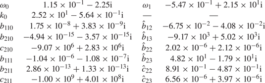
 $\omega _1$ may be determined. A particular solution for
 $\mathscr {A}=-1/2$,
 $R=1/\sqrt {2}$,
 $m=3$,
 $\delta _n=(6{\rm \pi} )^{-1}$,
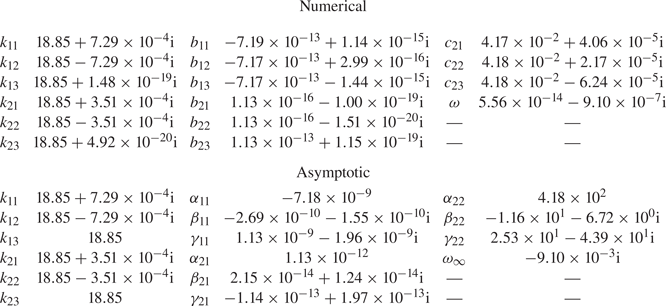
 $\eta =0$ is given in table 1.
Numerical evaluation of the coefficients of the low viscosity expansions in the case  $\mathscr {A} = -1/2$,
 $R = 1/\sqrt {2}$,
 $m = 3$,
 $\delta _n = (6{\rm \pi} )^{-1}$,
 $\eta = 0$.

In order to calculate the growth rate correction  $\omega _1$ we use the results of (A 1) to write four linear equations for
 $b_{111}$,
 $b_{211}$,
 $c_{211}$ and
 $\omega _1$. We define the functions
 \begin{gather} \hat{f}_I(r) = m \delta_n^2 k_0 \omega_0 I_{m}(k_0 r) + r (\omega_0 - 2) I_{m + 1}(k_0 r), \end{gather}
 \begin{gather}\hat{f}_K(r) = m \delta_n^2 k_0 \omega_0 K_{m}(k_0 r) - r (\omega_0 - 2) K_{m + 1}(k_0 r). \end{gather}
Hence we are able to show
 \begin{align} &\hat{f}_I(R) b_{111} = - \frac{\omega_1}{\omega_0^2 (\omega_0^2 - 4)} \left\{b_{110} \left[2 \hat{f}_I(R) \left[\omega_0 (\omega_0^2 - 4) + 4 m\right] \right.\right. \nonumber\\ &\qquad + \left.\left.2 k_0 \left[m \delta_n^2 ( - \omega_0 + 2 m) + 2 R^2\right] (\omega_0 - 2) \omega_0 I_m(k_0 R)\vphantom{\left\{b_{110} \left[2 \hat{f}_I(R) \left[\omega_0 (\omega_0^2 - 4) + 4 m\right] \right.\right.}\right] + 4\textrm{i} R \delta_n^2 k_0 \omega_0^2 (\omega_0 - 2)\vphantom{\left\{b_{110} \left[2 \hat{f}_I(R) \left[\omega_0 (\omega_0^2 - 4) + 4 m\right] \right.\right.}\right\}\nonumber\\ &\qquad + \textrm{e}^{-\textrm{i}{\rm \pi}/4} \left\{\vphantom{\left\{b_{110} \left[2 \hat{f}_I(R) \left[\omega_0 (\omega_0^2 - 4) + 4 m\right] \right.\right.} k_0 \omega_0 (m^2 \delta_n^2 + R^2) (\omega_0 - 2) \left[(b_{110} - b_{210}) I_m(k_0 R) - c_{210} K_m(k_0 R)\right] \right.\nonumber\\ &\qquad \left. + 2 m \left[\hat{f}_I(R) (b_{110} - b_{210}) - \hat{f}_K(R) c_{210}\right]\right\}\nonumber\\ &\qquad \times\left\{\omega_0^{3/2} R \left(\frac{1 - \mathscr{A}}{1 - \eta}\right)^{1/2} \left[1 + \left(\frac{1 - \mathscr{A}}{1 + \mathscr{A}}\right)^{1/2} \left(\frac{1 - \eta}{1 + \eta}\right)^{1/2}\right]\right\}^{-1}, \end{align}
 \begin{align} &\frac{1 - \mathscr{A}}{1 + \mathscr{A}}b_{111} - b_{211} - \frac{K_m(k_0 R)}{I_m(k_0 R)} c_{211} = \frac{\omega_1}{I_m(k_0 R) \omega_0 (\omega_0^2 - 4)} \left\{\left(b_{210} - \frac{1 - \mathscr{A}}{1 + \mathscr{A}} b_{110}\right) \right. \nonumber\\ &\quad \times \left. \left(4 k_0 R I_{m + 1}(k_0 R) + \left[3 \omega_0^2 + 4 (m - 1)\right] I_m(k_0 R)\right) \right. \nonumber\\ &\quad + \left. c_{210} \left[(3 \omega_0^2 + 4 (m - 1)) K_m(k_0 R) - 4 R k_0 K_{m + 1}(k_0 R)\right]\vphantom{\left\{b_{110} \left[2 \hat{f}_I(R) \left[\omega_0 (\omega_0^2 - 4) + 4 m\right] \right.\right.}\right\}, \end{align}
 \begin{align} &\hat{f}_I(R) b_{211} + \hat{f}_K(R) c_{211} = \frac{\omega_1}{\omega_0^2 (\omega_0^2 - 4)} \left\{\vphantom{(\hat{f}_K(R) c_{210} + (b_{210} - b_{110}) \hat{f}_I(R))}2 k_0 \omega_0 (\omega_0 - 2) \left[(m \delta_n^2 (\omega_0 - 2 m) - 2 R^2) \right.\right. \nonumber\\ &\qquad \left. \times (I_m(k_0 R) b_{210} + c_{210} K_m(k_0 R)) - 2 \textrm{i} R \delta_n^2 \omega_0\right]\nonumber\\ &\qquad - \left. (2 \hat{f}_I(R) b_{210} + 2 \hat{f}_K(R) c_{210}) (\omega_0 (\omega_0^2 - 4) + 4 m)\right\}\nonumber\\ &\qquad - \textrm{e}^{-\textrm{i}{\rm \pi}/4} \left\{\vphantom{\left\{b_{110} \left[2 \hat{f}_I(R) \left[\omega_0 (\omega_0^2 - 4) + 4 m\right] \right.\right.} k_0 \omega_0 (m^2 \delta_n^2 + R^2) (\omega_0 - 2) \left[c_{210} K_m(k_0 R) \right.\right.\nonumber\\ &\qquad \vphantom{(\hat{f}_K(R) c_{210} + (b_{210} - b_{110}) \hat{f}_I(R))}+ I_m(k_0 R) (b_{210} - b_{110})] \left. + 2 m (\,\hat{f}_K(R) c_{210} + (b_{210} - b_{110}) \hat{f}_I(R))\right\} \nonumber\\ &\qquad \times\left\{\vphantom{(\hat{f}_K(R) c_{210} + (b_{210} - b_{110}) \hat{f}_I(R))}\omega_0^{3/2} R \left(\frac{1 + \mathscr{A}}{1 + \eta}\right)^{1/2} \left[1 + \left(\frac{1 + \mathscr{A}}{1 - \mathscr{A}}\right)^{1/2} \left(\frac{1 + \eta}{1 - \eta}\right)^{1/2} \right] \right\}^{-1}, \end{align}
 \begin{align} &\hat{f}_I(1) b_{211} + \hat{f}_K(1) c_{211} = - \frac{2 \omega_1}{\omega_0^2 (\omega_0^2 - 4)} \left\{\vphantom{\left\{b_{110} \left[2 \hat{f}_I(R) \left[\omega_0 (\omega_0^2 - 4) + 4 m\right] \right.\right.}k_0 \omega_0 (\omega_0 - 2) \left[2 - m \delta_n^2 (\omega_0 - 2 m)\right] \right. \nonumber\\ &\quad \times \left. (I_m(k_0) b_{210} + K_m(k_0) c_{210}) + \left[\omega_0 (\omega_0^2 - 4) + 4 m\right] (\,\hat{f}_I(1) b_{210} + \hat{f}_K(1) c_{210})\right\}\nonumber\\ &\quad + \textrm{e}^{-\textrm{i}{\rm \pi}/4} \left\{k_0 \omega_0 (m^2 \delta_n^2 \!+\! 1) (I_m(k_0) b_{210} \!+\! K_m(k_0) c_{210}) (\omega_0 - 2) \!+\! 2 m (\,\hat{f}_I(1) b_{210} \!+\! \hat{f}_K(1) c_{210})\right\}\nonumber\\ &\quad \times\left\{\omega_0^{3/2} \left(\frac{1 + \mathscr{A}}{1 + \eta}\right)^{1/2}\right\}^{-1}. \end{align}
For parameters  $\mathscr {A} = -1/2$,
 $R = 1/\sqrt {2}$,
 $m = 3$,
 $\delta _n = (6{\rm \pi} )^{-1}$,
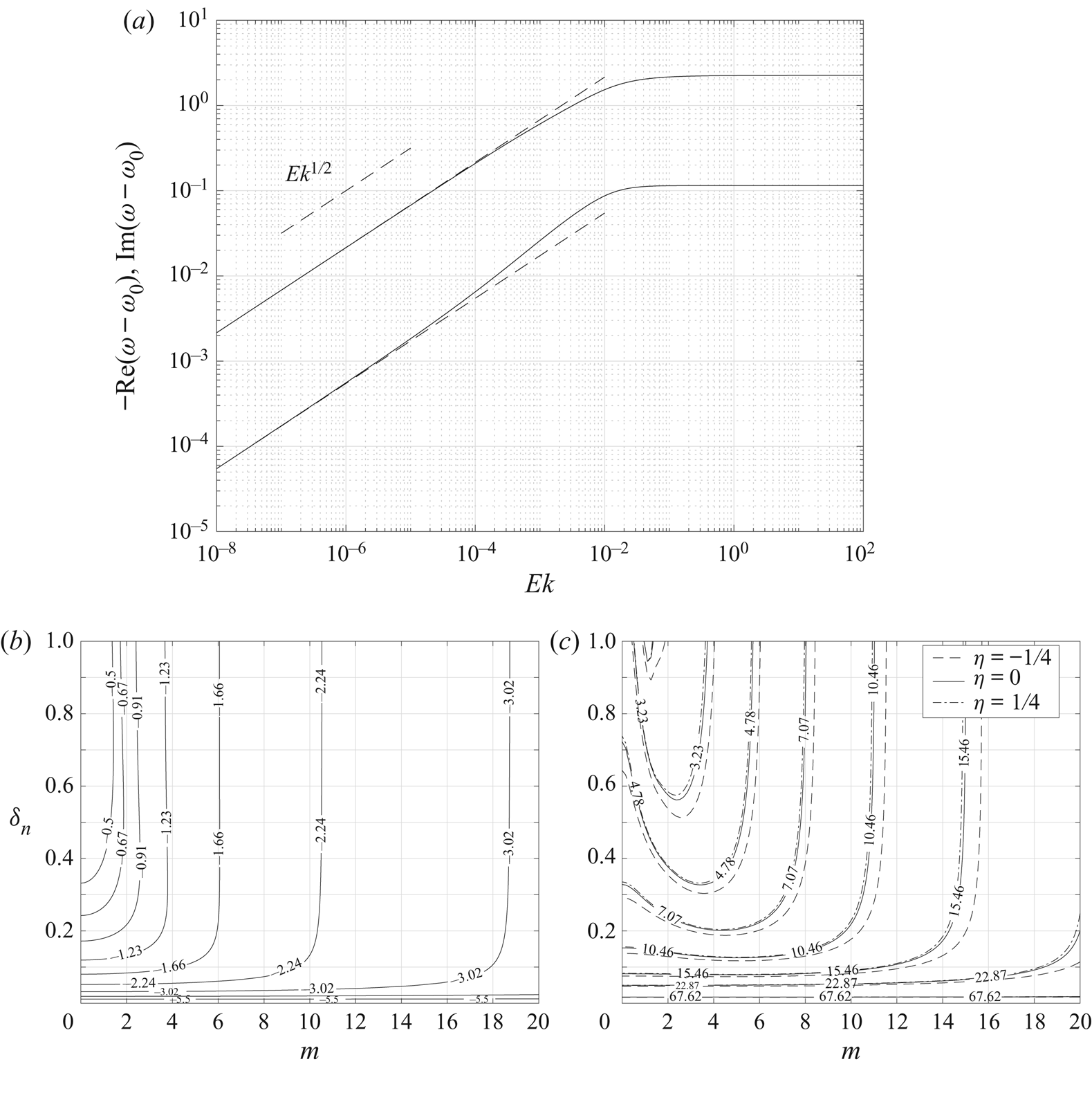
 $\eta =0$ values of the inviscid solution and the coefficients for the low viscosity asymptotic correction are quoted in table 1. For the same parameters, figure 2(a) is a plot of the difference between the exact eigenvalue
 $\omega$ for non-zero
 $Ek$, and the inviscid solution
 $\omega _0$. Both the real and imaginary parts of
 $\omega - \omega _0$ behave as
 $Ek^{1/2}$ as
 $Ek\to 0$, consistently with the asymptotic description. The upper solid line is
 $\textrm {Im}(\omega - \omega _0)$ which is positive as the effect of the fluid viscosity is to inhibit the growth of the perturbation. The lower solid line is
 $-\textrm {Re}(\omega - \omega _0)$. The dashed straight lines that coincide with the solid lines as
 $Ek\to 0$ are the correction
 $\omega _1 Ek^{1/2}$ calculated as described above by solving the linear system (2.45).
(a) The solid lines are the real and imaginary parts of the difference between the exact eigenvalue  $\omega$ calculated numerically and the inviscid eigenvalue
 $\omega _0$ (the upper line is the imaginary part, the lower line is the real part) for varying
 $Ek$. The parameters chosen were
 $\mathscr {A}=-1/2$,
 $R = 1/\sqrt {2}$,
 $m = 3$,
 $\delta _n = (6{\rm \pi} )^{-1}$. The imaginary part controls the growth of the instability and the correction to the inviscid growth rate behaves as
 $Ek^{1/2}$. The dashed lines that coincide with the numerical solution are the asymptotic correction calculated as described in § 2.3. (b) Contours of the imaginary part of the inviscid eigenvalue
 $\omega _0$ for
 $\mathscr {A}=-1/2$,
 $R = 1/\sqrt {2}$. As
 $m$ and
 $n$ increase the growth rate of the instability increases. (c) Contours of the imaginary part of the order
 $Ek^{1/2}$ correction,
 $\omega _1$ for
 $\mathscr {A}=-1/2$,
 $R = 1/\sqrt {2}$. The solid lines are for fluids of equal viscosity
 $\eta =0$, the dashed lines are the same value contours, but for an inner layer that is more viscous than the outer with
 $\eta = -1/4$, and the dot-dashed lines are the same value contours again, but for an outer layer that is more viscous than the inner with
 $\eta = 1/4$.

Figure 2(b) shows contours of  $\textrm {Im}(\omega _0)$, the growth rate of the inviscid solution, for the same Atwood number and initial interface location as figure 2(a). The contours show the behaviour of the inviscid system; the higher the azimuthal wavenumber,
 $m$, and the higher the axial wavenumber,
 $n$ (corresponding to lower values of
 $\delta _n$), the greater the growth rate in general. Figure 2(c) shows contours of the imaginary part of the coefficient
 $\omega _1$. The change in sign compared with
 $\textrm {Im}(\omega _0)$ shows that the viscous correction
 $\omega _1Ek^{1/2}$ acts to suppress the growth of the perturbation. Contours are shown for
 $\eta =0$ (solid) where the viscosity is the same in each layer,
 $\mu _1 = \mu _2$. Also shown are contours of
 $\eta = -1/4$ (dashed) where the inner layer is more viscous than the outer layer,
 $\mu _1 > \mu _2$, and
 $\eta = 1/4$ (dot-dashed) where the inner layer is less viscous than the outer layer,
 $\mu _1<\mu _2$. For the chosen parameters the plot shows that for a given Ekman number and Atwood number, having the more viscous fluid in the outer layer is more stable than having the more viscous fluid in the inner layer.
The effects of surface tension may be included in the low viscosity correction by using values of  $b_{110}$,
 $b_{210}$,
 $c_{210}$ and
 $\omega _0$ from the inviscid solution, including surface tension effects, in (2.45). No further modification of the linear system (2.45) for the remaining coefficients
 $b_{111}$,
 $b_{211}$
 $c_{211}$ and
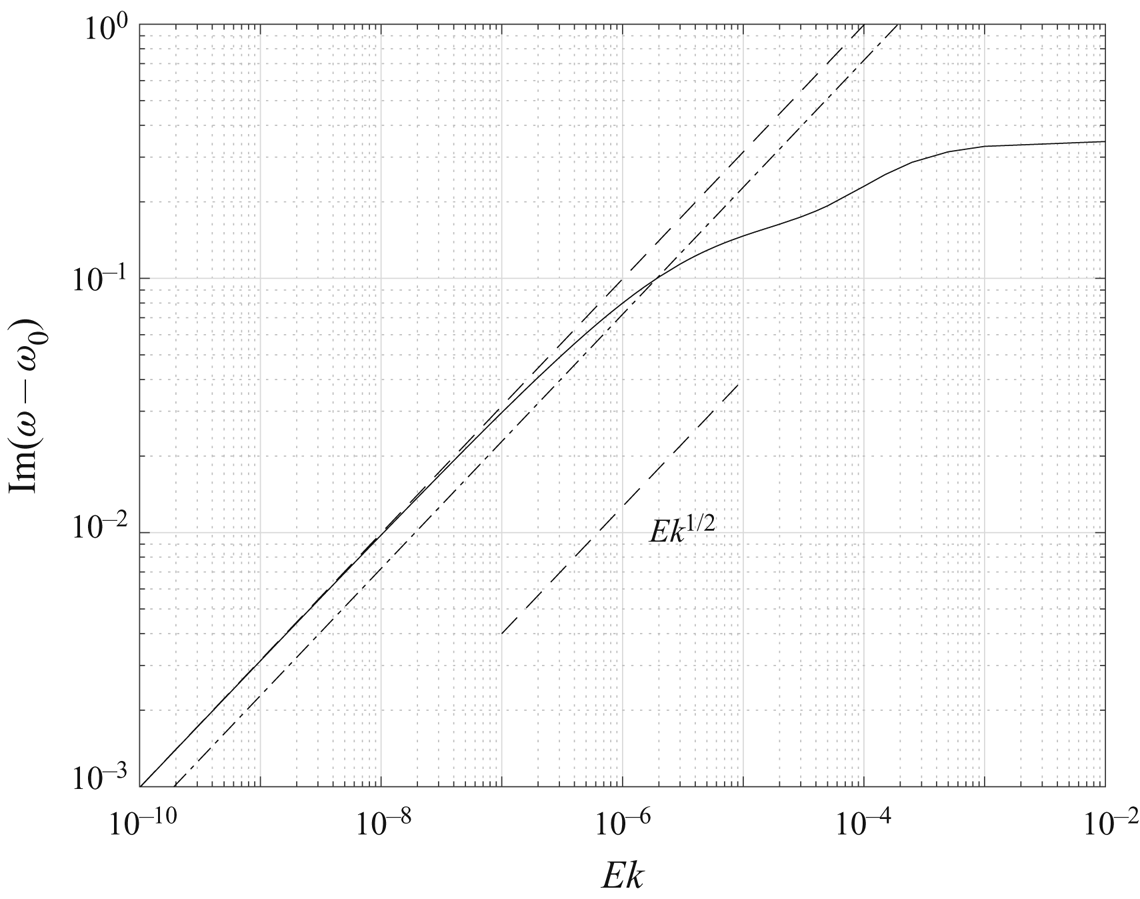
 $\omega _1$ is required. Figure 3 shows an example where
 $\mathscr {A} = -10^{-2}$,
 $R = 1/\sqrt {2}$,
 $m = 60$,
 $\delta _n = (10{\rm \pi} )^{-1}$,
 $\textit {We} = 10^6$,
 $\eta =0$. The solution without the correction for surface tension is shown dot-dashed. The asymptotic correction to the inviscid growth rate including the effects of surface tension is shown dashed and behaves as
 $Ek^{1/2}$, just as the solution without the correction for surface tension. As the surface-tension-corrected solution (dashed) lies above the correction without surface tension (dot-dashed) the effect of the surface tension is to inhibit the growth rate of the instability as might be anticipated on physical grounds.
The correction to the inviscid solution,  $\omega _0$ for
 $Ek\ll 1$. The chosen parameters were
 $\mathscr {A} = -10^{-2}$,
 $R = 1/\sqrt {2}$,
 $m = 60$,
 $\delta _n = (10{\rm \pi} )^{-1}$,
 $\eta =0$,
 $\textit {We} = 10^6$. The low viscosity asymptotic solution is
 $\omega \sim 7.58\times 10^{-3} - 3.47\times 10^{-1}\textrm {i} + (-6.70\times 10^{-1} + 9.94\times 10^1\textrm {i}) Ek^{1/2} + O(Ek)$. The positive imaginary part of the viscous correction shows viscosity damping the growth rate of the mode. The dot-dashed line is the low viscosity behaviour without the correction for surface tension. As the dashed line lies above the dot-dashed line the effect of the surface tension is to further dampen the growth rate of the instability.

2.4. High viscosity solutions
For very viscous fluids where  $Ek\gg 1$ the three solutions for
 $k^2$ to the governing wavenumber (2.9) behave as
 \begin{equation} k_{ij}^2 \sim \frac{1}{\delta_n^2} - \lambda_j\left(\frac{2\rho_i}{\delta_n\mu_i}\frac{1}{Ek}\right)^{2/3} + \frac{2\textrm{i}\rho_i\omega_\infty}{3\mu_i}\frac{1}{Ek^2} + O\left(\frac{1}{Ek^3}\right), \end{equation}
where  $\omega \sim \omega _\infty Ek ^{-1} + O(Ek^{-2})$ for the three values
 $j=1,2,3$ of
 $\lambda _j$ that satisfy
 $\lambda _j^3=-1$. Specifically we take
 \begin{equation} \lambda_j = \exp\left\{\textrm{i}\left[2j - 3\right]{\rm \pi}/3\right\} \quad{\rm for}\ j = 1, 2, 3. \end{equation}
We seek the leading-order growth rate  $\omega _\infty Ek^{-1}$ and so must determine the coefficients
 $b_{ij}$ and
 $c_{2j}$ for
 $i=1,2$ and
 $j=1,2,3$ to a high enough order of accuracy that
 $\omega _\infty$ may itself be determined. For each of the nine coefficients, as with (2.46), this requires finding the first three terms of the asymptotic expansion. Motivated by observations from numerical solutions we pose, for
 $i=1, 2$, that the coefficients be of the form
 \begin{gather} b_{i1} \sim \alpha_{i1}\frac{1}{Ek} + \beta_{i1}\frac{\lambda_1}{Ek^{4/3}} + \gamma_{i1}\frac{\lambda_3}{Ek^{5/3}} + O\left(\frac{1}{Ek^2}\right), \end{gather}
 \begin{gather}b_{i2} \sim \alpha_{i1}\frac{1}{Ek} + \beta_{i1}\frac{\lambda_3}{Ek^{4/3}} + \gamma_{i1}\frac{\lambda_1}{Ek^{5/3}} + O\left(\frac{1}{Ek^2}\right), \end{gather}
 \begin{gather}b_{i3} \sim \alpha_{i1}\frac{1}{Ek} + \beta_{i1}\frac{\lambda_2}{Ek^{4/3}} + \gamma_{i1}\frac{\lambda_2}{Ek^{5/3}} + O\left(\frac{1}{Ek^2}\right), \end{gather}
and similarly for  $c_{2j}$ for
 $j=1,2,3$. This form of approximation to the coefficients replaces the nine unknown general coefficients
 $b_{ij}$ and
 $c_{2j}$ with nine unknown coefficients in the large
 $Ek$ expansion;
 $\alpha _{11}$ in the inner layer,
 $\alpha _{21}$ and
 $\alpha _{22}$ in the outer layer, and similarly for
 $\beta$ and
 $\gamma$. The leading and second-order boundary and matching equations at
 $O(Ek^{-4/3})$ and
 $O(Ek^{-5/3})$ are automatically satisfied, leaving a system of ten linear equations (see (B 1)–(B 10) in appendix B) in the nine unknown coefficients
 $\alpha$,
 $\beta$ and
 $\gamma$ and the eigenvalue
 $\omega _\infty$ that may be solved by standard methods.
Here we give the solution for  $\omega _\infty$ in the special case of equal viscosity in each fluid layer,
 $\eta =0$ and no surface tension. The general expression for arbitrary
 $\eta$ and surface tension is considerably more cumbersome, but may be found from (B 1)–(B 10). We express
 $\omega _\infty$ in terms of the following functions:
 \begin{gather} F_1(r) = 2 \delta_n r K_{m+1}\left(\frac{r}{\delta_n}\right) + \left[\left(m-2\right)m\delta_n^2 + r^2\right] K_m\left(\frac{r}{\delta_n}\right), \end{gather}
 \begin{gather} F_2(r) = -\left[(m-2)\frac{m\delta_n^2}{2} + \frac{R^2 r^2}{2}\right]K_{m+1}\left(\frac{1}{\delta_n}\right) +m\delta_n\left[(m-2)m\delta_n^2 \!+\! \frac{R^2 + r^2}{2}\right] K_m\left(\frac{1}{\delta_n}\right), \end{gather}
 \begin{gather} F_3(r) = 2\left(m^2-4\right)m^2\delta_n^4+\left[m^2(r^2 + R^2) + 2m(1 + r^2 + R^2)\right]\delta_n^2 - R^2\left(1-\frac{r^2}{2}\right). \end{gather}
We also define the constants  $G_1$ and
 $G_2$ in terms of the parameters
 $m$,
 $\delta _n$ and
 $R$
 \begin{align} G_1 &= \frac{1}{2}I^3_{m+1}\left(\frac{1}{\delta_n}\right) + \frac{3m+2}{2}\delta_n I_{m}\left(\frac{1}{\delta_n}\right)I^2_{m+1}\left(\frac{1}{\delta_n}\right) \nonumber\\ &\quad + \left[(m + 2)m\delta_n^2-\frac{1}{2} \right] I^2_{m}\left(\frac{1}{\delta_n}\right) I_{m+1}\left(\frac{1}{\delta_n}\right) - \frac{m\delta_n}{2}I^3_{m}\left(\frac{1}{\delta_n}\right), \end{align}
 \begin{equation} G_2 = I_{m+1}\left(\frac{R}{\delta_n}\right) K_{m}\left(\frac{R}{\delta_n}\right)+K_{m+1}\left(\frac{R}{\delta_n}\right) I_{m}\left(\frac{R}{\delta_n}\right). \end{equation}
Finally, we define the following five constants in terms of the  $m$,
 $\delta _n$ and
 $R$ and the functions
 $F_1$,
 $F_3$ and constants
 $G_1$ and
 $G_2$:
 \begin{gather} H_1 = \left[(m+2)R^2-m\right]\delta_n K_{m+1}\left(\frac{1}{\delta_n}\right) + \left[(m-2)m\delta_n^2 + R^2\right]K_m\left(\frac{1}{\delta_n}\right), \end{gather}
 \begin{gather}H_2 = \left[(m+2)m\delta_n^2 + R^2\right] R K_{m+1}\left(\frac{R}{\delta_n}\right) - 2m \delta_n F_1(R), \end{gather}
 \begin{gather}H_3 = \left[1+(m+2)^2\delta_n^2\right] K_{m+1}\left(\frac{1}{\delta_n}\right) + 2\delta_n K_m\left(\frac{1}{\delta_n}\right), \end{gather}
 \begin{align} H_4 &= -m \delta_n \left[(m-2)m\delta_n^2 + R^2\right] K_{m+1}\left(\frac{1}{\delta_n}\right)\nonumber\\ &\quad +\frac{1}{2}\left[4(m-2)m^3\delta_n^4 + (4R^2+1)m^2\delta_n^2+R^4\right]K_m\left(\frac{1}{\delta_n}\right), \end{align}
 \begin{align} H_5 &= \frac{R^2}{2}\left\{\left[1+(m+2)m\delta_n^2\right]K_{m+1}\left(\frac{1}{\delta_n}\right) + (m+2)\delta_n F_1(1)\right\} I^2_{m+1}\left(\frac{R}{\delta_n}\right)\nonumber\\ &\quad + R\left\{F_3(0) K_m\left(\frac{1}{\delta_n}\right) - \delta_n \left[(m^2-4)m \delta_n^2 + 2 R^2(m+1) -m\right]K_{m+1}\left(\frac{1}{\delta_n}\right)\right\}\nonumber\\ &\quad \times I_m\left(\frac{R}{\delta_n}\right)I_{m+1}\left(\frac{R}{\delta_n}\right)\nonumber\\ &\quad +\left\{ \frac{1}{2}\left(\left[(m+2)m\delta_n^2 - R^2\right](1-R^2)-F_3(0) \right) K_{m+1}\left(\frac{1}{\delta_n}\right) \right. \nonumber\\ &\quad \left. +m \delta_n \left[F_3(R)-\frac{m\delta_n^2}{2}(m + 2)\right] K_m\left(\frac{1}{\delta_n}\right)\right\} I^2_m\left(\frac{R}{\delta_n}\right). \end{align}
We may now write the coefficient of the asymptotic growth rate as
 \begin{align} \omega_\infty &= \frac{\textrm{i} \mathscr{A}}{R G_1 G_2}\left\{ \left[m \delta_n I^2_m\left(\frac{1}{\delta_n}\right)F_2(R) - H_4 I^2_{m+1}\left(\frac{1}{\delta_n}\right)\right] I^2_m\left(\frac{R}{\delta_n}\right) \right. \nonumber\\ &\quad \left. +R\left[\left(m \delta_n H_1 I_m\left(\frac{1}{\delta_n}\right)^2 - 2F_2(1) I^2_{m+1}\left(\frac{1}{\delta_n}\right)\right) I_m\left(\frac{R}{\delta_n}\right) +G_1 F_1(R)\right]I_{m+1}\left(\frac{R}{\delta_n}\right) \right. \nonumber\\ &\quad \left. -\frac{R^2}{2}\left[ m \delta_n H_3 I^2_m\left(\frac{1}{\delta_n}\right) + F_1(1) I^2_{m+1}\left(\frac{1}{\delta_n}\right)\right] I_{m+1}\left(\frac{R}{\delta_n}\right)^2 \right. \nonumber\\ &\quad \left. - G_1 H_2 I_m\left(\frac{R}{\delta_n}\right) - H_5 I_{m+1}\left(\frac{1}{\delta_n}\right) I_m\left(\frac{1}{\delta_n}\right)\right\}. \end{align}
As with the special  $\eta =0$ case above, for arbitrary
 $\eta$ the leading-order growth rate in the absence of surface tension,
 $\omega _\infty Ek ^{-1}$, is linear in the Atwood number,
 $\mathscr {A}$, and its dependence upon the aspect ratio
 $\delta$ and the axial wavenumber
 $n$ is only through
 $\delta _n$. A solution for the purposes of verification of any implementation is provided in table 2.
Numerical and asymptotic approximations in the high viscosity regime for the unknown coefficients and growth rates for parameters  $Ek = 10^4$,
 $\mathscr {A} = -1/2$,
 $R = 1/\sqrt {2}$,
 $\delta _n = (6{\rm \pi} )^{-1}$,
 $m = 3$,
 $\eta =0$. The difference in order of magnitude of coefficients requires a high degree of numerical accuracy to be used. The agreement between the numerical value of
 $\omega$ and the asymptotic value
 $\omega _\infty \,Ek^{-1}$ is good.

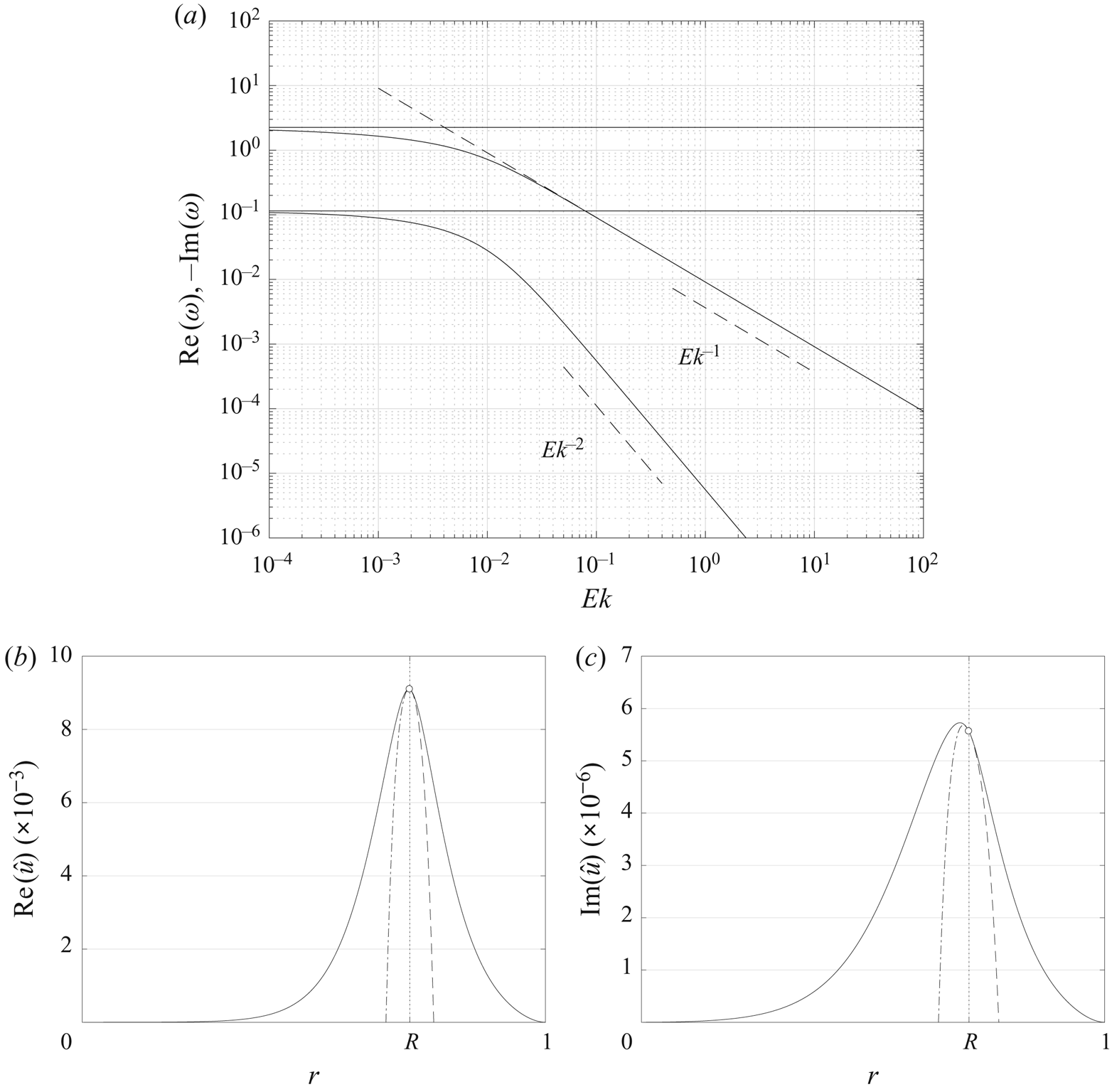
Figure 4(a) shows the behaviour of  $\omega$ (solid curves) for parameters
 $\mathscr {A} = -1/2$,
 $R = 1/\sqrt {2}$,
 $m = 3$,
 $\delta _n = (6{\rm \pi} )^{-1}$,
 $\eta = 0$ and no surface tension. As
 $Ek\to \infty$, the imaginary part of
 $\omega$ behaves as
 $Ek^{-1}$, whereas the real part behaves as
 $Ek^{-2}$. The precession, controlled by
 $ {\rm Re}(\omega )$, is suppressed more rapidly than the growth of the perturbation as the Ekman number is increased. The horizontal solid lines are the imaginary (upper) and real (lower) parts of the inviscid solution
 $\omega _0$. It can be seen that as
 $Ek\to 0$ the solid curves tend toward the inviscid solution since
 $\omega \to \omega _0$. The dashed line that coincides with the upper solid curve as
 $Ek\to \infty$ is the asymptotic high viscosity approximation
 $-\textrm {Im}(\omega _\infty Ek ^{-1})$ given by (2.52). This approximation is an estimate of the instability in the high viscosity limit and can be seen to be in good agreement with the numerical value as
 $Ek\to \infty$.
Numerical solutions for  $\mathscr {A}=-1/2$,
 $R = 1/\sqrt {2}$,
 $\eta = 0$,
 $m = 3$,
 $\delta _n = (6{\rm \pi} )^{-1}$. (a) The real and (negative) imaginary parts of the eigenvalue
 $\omega$. The imaginary part controls the growth of the instability and behaves as
 $Ek^{-1}$ as
 $Ek\to \infty$. The dashed line that coincides with the numerical solution is calculated using (2.52). The upper horizontal solid line is the imaginary part of the inviscid solution given by (2.31). The real part of the solution behaves as
 $Ek^{-2}$ as
 $Ek\to \infty$ and again tends to the real part of the inviscid solution shown by the lower solid horizontal line as
 $Ek\to 0$. (b) The real part of
 $\hat {u}$ and (c) the imaginary part of
 $\hat {u}$ where the horizontal velocity is written as
 $u = \hat {u}(r)\cos (\delta _n^{-1}[z - \delta ])\exp ({\textrm {i}(m\theta + \omega t)})$ and here
 $Ek=1$. The transitions between the inner and outer solutions occur at
 $r=R$ (vertical dotted line) and are indicated by the white circles.

Figures 4(b) and 4(c) show typical profiles of the radial dependence of the radial velocity field. Writing  $u = \hat {u}(r)\cos (\delta _n^{-1}[z - \delta ])\exp ({\textrm {i}(m\theta + \omega t)})$ the real and imaginary parts of
 $\hat {u}$ are shown in figures 4(b) and 4(c), respectively. The inner layer solutions extend from
 $r=0$ to
 $r = R$ and are shown as solid lines. At
 $r = R$ the inner solution matches smoothly onto the outer solution as a result of the requirements of continuity of velocity and stress at the interface. The points at which the two solutions match, at
 $r=R$, is indicated by a white circle. The outer solution extends from
 $r = R$ to
 $r=1$ and is also shown as a solid line. The continuation of the inner layer solution into the outer layer is shown dashed and the continuation of the outer layer solution into the inner layer is shown dot-dashed.
In the absence of surface tension,  $\omega _\infty$ is proportional to
 $\mathscr {A}$ and hence the most unstable mode pairing
 $(m, n)$ is a function of
 $R$,
 $\delta$ and
 $\eta$ alone. Furthermore, the dependence of
 $\omega _\infty$ on
 $\delta$ and
 $n$ is through
 $\delta _n$ only. Hence, provided we are in the high viscosity regime,
 $Ek\gg 1$, and surface tension is negligible, we have that the most unstable mode pairing
 $(m, n)$, for a given aspect ratio
 $\delta$ is determined by the interface location,
 $R$, and the viscosity contrast
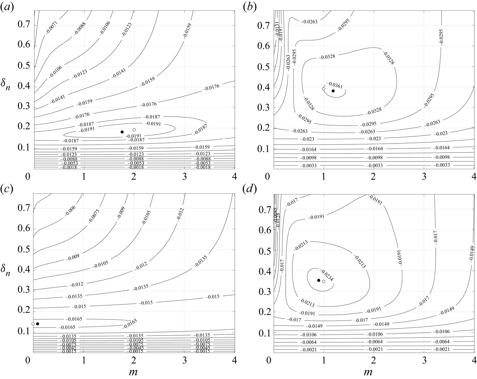
 $\eta$ alone. Figure 5 shows contours of
 $\textrm {Im}(\omega _\infty )$ for different choices of
 $R$ and
 $\eta$. The minimum value of
 $\textrm {Im}(\omega _\infty )$ in each case is shown with a black circle (treating
 $\omega _\infty$ as continuous in
 $m$) and the most unstable mode of growth is shown with a white circle (treating
 $\omega _\infty$ as dependent on
 $m\in \mathbb {N}$).
Contours of  $\textrm {Im}(\omega )$, the most unstable mode in the absence of surface tension for: (a)
 $\eta =0$,
 $R = 1/\sqrt {2}$; (b)
 $\eta =-9/11$,
 $R = 1/\sqrt {2}$; (c)
 $\eta =9/11$,
 $R = 1/\sqrt {2}$; (d)
 $\eta =0$,
 $R = 1/2$ as a function of azimuthal wavenumber,
 $m$, and
 $\delta _n$. The minimum value in each case is shown by a black circle. The minimum value with
 $m$ constrained to integer values is shown by a white circle.

In figure 5(a) the parameters are  $R = 1/\sqrt {2}$ (equal volumes of fluid in each layer) and
 $\eta =0$ (no viscosity contrast between the two layers,
 $\mu _1 = \mu _2$). Treating
 $\omega _\infty$ as continuous in
 $m$, the minimum value of
 $\textrm {Im}(\omega _\infty )$ is located at
 $m = 1.76$,
 $\delta _n = 0.18$. However, for the most unstable mode of growth we require
 $m\in \mathbb {N}$ and the minimum subject to this constraint is located at
 $m = 2$,
 $\delta _n = 0.19$, an elliptical deformation of the inner fluid layer about the axis.
In figures 5(b) and 5(c) the location of the interface is kept as in figure 5(a), but the viscosity contrast between the layers is varied. In figure 5(b)  $\eta = -9/11$ meaning that the inner layer is a factor of 10 times more viscous than the outer layer. The minimum of
 $\textrm {Im}(\omega _\infty )$ is located at
 $m = 1.19$,
 $\delta _n = 0.38$ and constraining
 $m$ to integer values gives the most unstable mode at
 $m=1$,
 $\delta _n = 0.39$. This corresponds to a translational motion of the inner layer away from the axis toward the outer boundary.
In figure 5(c)  $\eta = 9/11$ meaning that the outer layer is a factor of 10 times more viscous than the inner layer. The minimum of
 $\textrm {Im}(\omega _\infty )$ is located at
 $m = 0.09$,
 $\delta _n = 0.14$ and corresponds to a most unstable mode given by
 $m=0$,
 $\delta _n = 0.14$. This indicates that the instability develops as a varicose instability, the outer layer is sufficiently viscous that it does not allow the inner layer to move its centre of mass radially and the two fluids tend to change places initially through the growth of axial perturbations alone. The value of
 $\min\{\textrm {Im}(\omega )\}$ in figure 5(c) is greater than the value of
 $\min\{\textrm {Im}(\omega )\}$ in figure 5(b) indicating that, as in the low viscosity limit, for a given Ekman number and Atwood number having the more viscous fluid in the outer layer is more stable than having the more viscous fluid in the inner layer.
Figure 5(d) shows contours of  $\textrm {Im}(\omega _\infty )$ for layers of equal viscosity (
 $\eta =0$) but with the interface at
 $R = 1/2$. As with figure 5(b), a preference is shown for a translational motion of the inner layer to the outer boundary as the two fluids start to move.
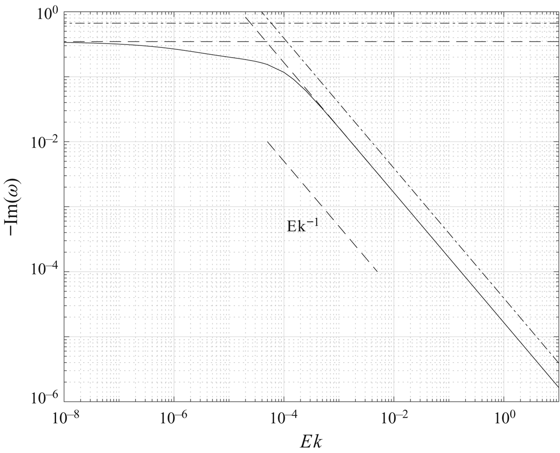
Figure 6 is a comparison of the high viscosity solution with and without surface tension. The solution without the correction for surface tension is shown dot-dashed. The high viscosity asymptotic solution for the growth rate including the effects of surface tension is shown dashed and behaves as  $Ek^{-1}$ (just as the solution without the correction for surface tension). As the surface tension solution (dashed) lies below the solution without surface tension (dot-dashed) the effect of the surface tension is as in the low-viscosity case, to inhibit the growth rate of the instability.
The growth rate  $-\textrm {Im}(\omega )$ for the chosen parameters
 $\mathscr {A} = -10^{-2}$,
 $R = 1/\sqrt {2}$,
 $m = 60$,
 $\delta _n = (10{\rm \pi} )^{-1}$,
 $\eta =0$,
 $\textit {We} = 10^6$ (the same parameters as in figure 3). The high-viscosity asymptotic solution is
 $\omega \sim -1.65\times 10^{-5}\textrm {i}Ek^{-1} + O(Ek^{-2})$ shown as the diagonal dashed line. The horizontal dashed and dot-dashed lines are the inviscid solution with and without the correction for surface tension, respectively. The dot-dashed diagonal line is the high viscosity asymptotic solution without the correction for surface tension. As the dot-dashed line lies above the dashed line, as with the low-viscosity case, the effect of the surface tension is to dampen the growth rate of the instability.

3. Numerical simulation of instability
The numerical simulations of the instability were performed using the volume-of-fluid method implemented in the ‘interFoam’ solver which is part of the OpenFOAM distribution (Weller et al. Reference Weller, Tabor, Jasak and Fureby1998). The solver is reviewed and discussed in Deshpande, Anumolu & Trujillo (Reference Deshpande, Anumolu and Trujillo2012) and the modifications for use in rotating frames of reference are described in Scase & Hill (Reference Scase and Hill2018). A volume-of-fluid approach is used to solve the continuity equation
 \begin{equation} \frac{\partial\rho}{\partial t} + \boldsymbol{\nabla}\boldsymbol{\cdot}\left(\rho\boldsymbol{u}\right) = 0 \end{equation}
and the rotating momentum equation
 \begin{equation} \frac{\partial}{\partial t}\left(\rho\boldsymbol{u}\right) + \boldsymbol{\nabla}\boldsymbol{\cdot}\left(\rho\boldsymbol{u}\boldsymbol{u}\right) = -\boldsymbol{\nabla} p - \rho\boldsymbol{\varOmega}\times\left(\boldsymbol{\varOmega}\times\boldsymbol{x}\right) - 2\rho\boldsymbol{\varOmega}\times\boldsymbol{u} +\left[\boldsymbol{\nabla}\boldsymbol{\cdot}\left(\mu\nabla\boldsymbol{u}\right) + \boldsymbol{\nabla}\boldsymbol{u}\boldsymbol{\cdot}\boldsymbol{\nabla}\mu\right]. \end{equation}
The solution domain is taken to be a wedge where  $r\in [0, 1]$,
 $\theta \in [-2{\rm \pi} /m, 2{\rm \pi} /m]$ and
 $z\in [-1/2, 1/2]$. For the simulations shown the domain is split into approximately
 $250\times 25\times 250$ cells. The total number of control volumes was greater than
 $1.5\times 10^6$ and the temporal step size was
 ${\rm \Delta} t = 2.5\times 10^{-3}$. The interface is initially perturbed with an azimuthal wavenumber
 $m=60$ and an axial wavenumber
 $n = 10$. The initial condition in the numerical simulations is that the flow starts from rest in the rotating frame.
Two series of simulations were run, one series in the low viscosity regime and one series in the high viscosity regime. The flow domain had a dimensional radius and height of 10 cm giving an aspect ratio  $\delta = 1/2$, the initial unperturbed position of the interface was taken to be
 $R = 1/\sqrt {2}$ such that the volume of each phase was equal. In the low viscosity regime the two fluid phases had properties similar to those of water with a reference density of
 $10^3\ \textrm {kg}\ \textrm {m}^{-3}$ and both layers a dynamic viscosity of
 $10^{-3}\ \textrm {kg}\ \textrm {m}^{-1}\ \textrm {s}^{-1}$. The Atwood number was chosen to be an unstable
 $\mathscr {A}=-10^{-2}$, and the rotation rate was set at
 $8{\rm \pi} \ \textrm {rad}\ \textrm {s}^{-1}$ or 240 r.p.m. The theoretical predictions are that the non-dimensional inviscid growth rate is given by
 $-\textrm {Im}(\omega _0) = 0.67$, the exact growth rate in the low viscosity regime is
 $-\textrm {Im}(\omega ) = 0.54$, and the low viscosity asymptotics give a predicted growth rate described by
 $-\textrm {Im}(\omega _0 + \omega _1Ek^{1/2}) = 0.52$.
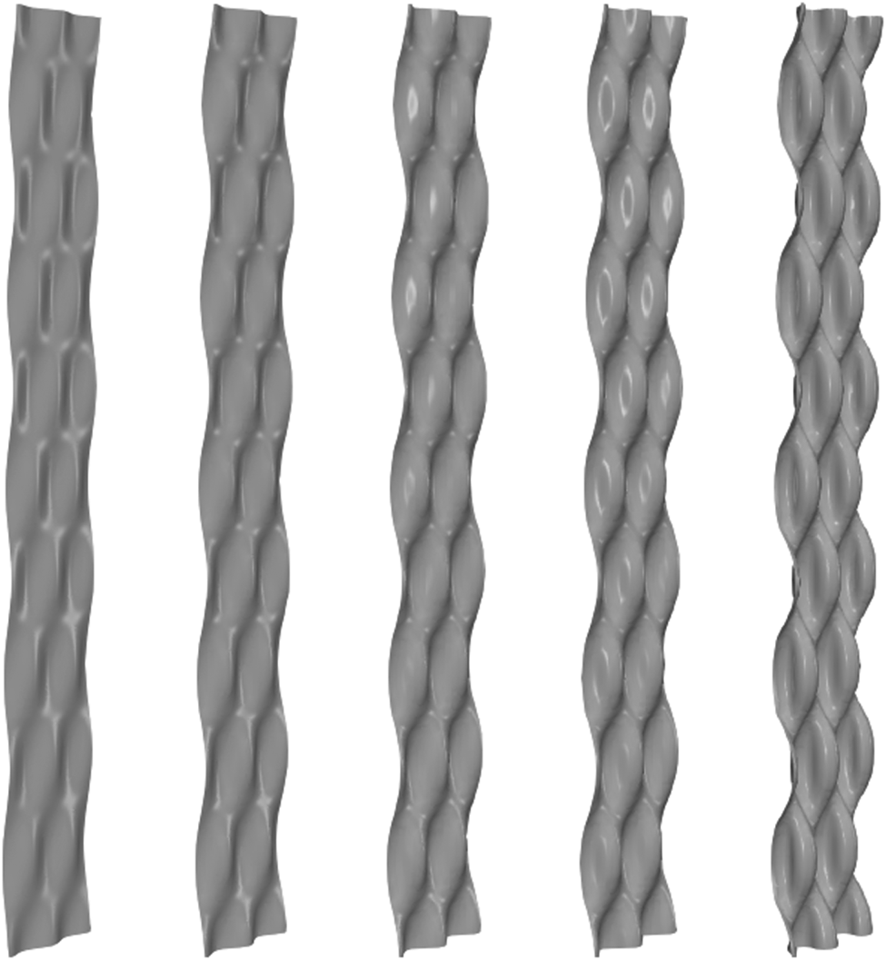
Figure 7 shows the developing interface, defined to be the surface where  $\rho = \rho _0$, between the two fluid phases at non-dimensional times
 $t = 0$,
 $1.38$,
 $2.14$,
 $2.51$ and
 $3.64$ from left to right, respectively, for fluids in the low viscosity regime. The
 $r=0$ axis is to the left of the shown contour as drawn. For
 $t \gtrsim 2.5$, nonlinear effects start to be observed at the interface.
The developing instability at the interface for fluids in the low viscosity regime. The simulation parameters were  $\mathscr {A} = -0.01$,
 $R = 1/\sqrt {2}$,
 $\delta _n = (10{\rm \pi} )^{-1}$,
 $m = 60$,
 $\eta = 0$,
 $Ek = 3.98\times 10^{-6}$. The Ekman number follows from a dimensional rotation rate of the system of
 $8{\rm \pi} \ \textrm {rad}\ \textrm {s}^{-1}$ for two fluids with mean dynamic viscosity
 $\mu _0 = 10^{-3}\ \textrm {kg}\ \textrm {m}^{-1}\ \textrm {s}^{-1}$ and mean density
 $\rho _0 = 10^3\ \textrm {kg}\ \textrm {m}^{-3}$ in a domain of radial extent
 $a = 0.1$ m. The non-dimensional times shown are
 $t=0$,
 $1.38$,
 $2.14$,
 $2.51$ and
 $3.64$ from left to right.

In the high viscosity regime the two fluid phases had properties similar to those of a dense and viscous black treacle or molasses. The reference fluid density was  $1.5\times 10^3\ \textrm {kg}\ \textrm {m}^{-3}$ and the dynamic viscosity in each layer was taken as
 $10\ \textrm {kg}\ \textrm {m}^{-1}\ \textrm {s}^{-1}$, the Atwood number was unchanged at
 $\mathscr {A} = -10^{-2}$. The rotation rate was
 $2{\rm \pi} \ \textrm {rad}\ \textrm {s}^{-1}$ or 60 r.p.m. The exact theoretical growth rate in the high viscosity regime is given by
 $-\textrm {Im}(\omega ) = 3.68\times 10^{-4}$ and the high viscosity asymptotics predict
 $-\textrm {Im}(\omega _\infty Ek^{-1}) = 3.68\times 10^{-4}$.
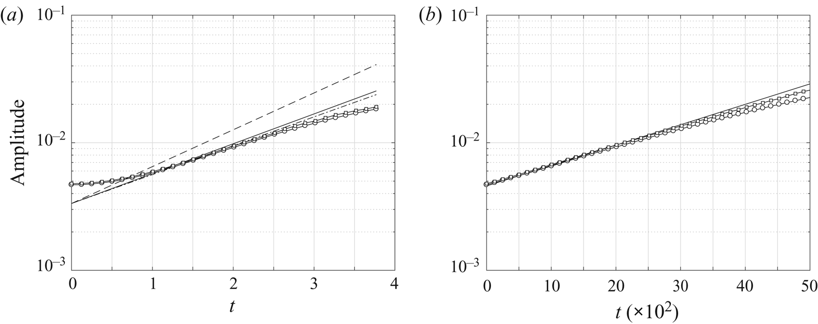
The simulated and predicted growth rates of the perturbation to the interface in the low viscosity regime are compared in figure 8(a). The amplitude of the simulated perturbation to the interface is shown by the circular and square data points, the circular data points are the amplitude of the axial perturbations and the square data points are the amplitude of the azimuthal perturbations. The dashed line is the predicted amplitude using the inviscid model of § 2.2 that gives  $\omega _0 = 0.01 - 0.67\textrm {i}$ for the chosen parameters
 $\mathscr {A} = -10^{-2}$,
 $\delta _n = (10{\rm \pi} )^{-1}$,
 $m = 60$,
 $R = 1/\sqrt {2}$. As anticipated on physical grounds, due to the absence of viscosity, the inviscid model overpredicts the growth rate of the perturbation. The dashed-dot line is the asymptotic correction to the inviscid prediction using the low-viscosity solution in § 2.3. With the chosen parameters the simulated Ekman number is
 $Ek = 3.98\times 10^{-6}$ and the low-viscosity prediction using § 2.3 is
 $\omega \sim 0.01-0.52\textrm {i}$. The exact eigenvalue calculated numerically is
 $\omega = 0.01-0.54\textrm {i}$, and this solution is shown as the solid line. As is observed, once the instability starts to grow its growth rate during the linear phase is well-predicted by both the exact solution and the low-viscosity asymptotic model.
The amplitude of the interfacial perturbation with non-dimensional time for parameters  $\mathscr {A} = -10^{-2}$,
 $\delta _n = (10{\rm \pi} )^{-1}$,
 $m = 60$,
 $\eta = 0$. The data points are from the numerical simulation where the amplitude of the perturbation has been calculated by considering the axial perturbation through a meridional plane (circular data points) and the azimuthal perturbation through a horizontal plane (square data points). (a) The low viscosity regime: the dashed line is the predicted amplitude from the inviscid model
 $\omega _0 = 0.01 - 0.67\textrm {i}$, the dot-dashed line is the low Ekman number asymptotic prediction
 $\omega \sim 0.01 - 0.52\textrm {i}$ and the solid line is the exact solution from the full model
 $\omega = 0.01 - 0.54\textrm {i}$. (b) The high viscosity regime: the solid line is the exact solution calculated from the model
 $\omega = 9.61\times 10^{-9}-3.68\times 10^{-4}\textrm {i}$, the dashed line is the amplitude predicted by the high viscosity asymptotics (2.52),
 $\omega _\infty Ek ^{-1} = -3.68\times 10^{-4}\textrm {i}$, but cannot be distinguished from the exact solution at the scale shown.

Figure 8(b) compares the predicted and observed amplitudes of the interfacial perturbation in a high viscosity regime. The circular and square data points indicate the amplitude of the axial and azimuthal perturbations, respectively, as in figure 8(a). The solid line follows the exact numerical growth rate  $-\textrm {Im}(\omega ) = 3.68\times 10^4$. Also plotted is a dashed line following the high viscosity asymptotic prediction
 $-\textrm {Im}(\omega _\infty Ek ^{-1})$, but at the scale shown this lies on top of the exact numerical solution. A good agreement is observed between the predicted growth rate and the observed amplitude of the simulated perturbation.
4. Rotating viscous column
A special case of the configuration of fluids that has been considered so far is that of the rotating viscous liquid column. This situation occurs in the absence of an outer fluid layer, in the limit  $\rho _2\to 0$,
 $\mu _2\to 0$. We refer to this limit as the ‘viscous column’ limit which may be equivalently taken as
 $\mathscr {A}\to -1$,
 $\eta \to -1$. The behaviour of liquid columns has received considerable attention in the past, building from the initial work of Rayleigh (Reference Rayleigh1879, Reference Rayleigh1892) to the inclusion of rotation (Hocking & Michael Reference Hocking and Michael1959) and viscosity (Hocking Reference Hocking1960). More recently a linear stability analysis of a uniformly rotating viscous liquid column in the absence of gravity was considered by Kubitschek & Weidman (Reference Kubitschek and Weidman2007a) together with a companion experimental study (Kubitschek & Weidman (Reference Kubitschek and Weidman2007b), where gravity was present) following on from the inviscid studies of Weidman et al. (Reference Weidman, Goto and Fridberg1997) and Weidman (Reference Weidman1994). In Kubitschek & Weidman (Reference Kubitschek and Weidman2007a) the authors investigated an analytical description of the linear stability of a uniformly rotating viscous column numerically, including showing how their results tend to the established inviscid results in the limit
 $Ek\to 0$. The authors investigated the preferred mode of instability of a uniformly rotating viscous column as a function of the Ekman number,
 $Ek$, and the Weber number,
 $\textit {We}$ (Reynolds number,
 $Re$, and Hocking parameter,
 $L$, in their notation). Through an extensive, careful numerical investigation they were able to establish which mode of instability had the greatest growth rate for a given value of
 $Ek$ and
 $\textit {We}$ and conjectured an asymptotic form of the boundary between the two most unstable modes (an axisymmetric mode and a spiral mode) in the limit of high viscosity and high surface tension (see figure 13 Kubitschek & Weidman (Reference Kubitschek and Weidman2007a), figure 1 Kubitschek & Weidman (Reference Kubitschek and Weidman2007b): the boundary is denoted
 $T_{01}$).
Here we are able to compare our general asymptotic approximations derived in § 2 with the special case of a single uniformly rotating viscous column layer. By modifying the dependence of the axial wavenumber and Weber number, such that they depend on the Ekman number, we are able to confirm the conjectured asymptotic form of the  $T_{01}$ boundary identified by Kubitschek & Weidman (Reference Kubitschek and Weidman2007a) and find an expression for the boundary that is in good agreement with their numerical estimate.
The boundary between the preferred modes of instability depends upon the growth rate of the most unstable mode in each regime only. The wavelengths of the associated most unstable modes either side of the boundary may be quite different, as may the precession associated with the mode.
In the case of a single fluid layer, the governing system of equations described in § 2 is reduced. The six coefficients,  $b_{2j}$ and
 $c_{2j}$, describing the behaviour of the outer layer may all be considered identically zero as the outer layer is not present. The three boundary conditions on
 $r=1$ for the outer layer, (2.11a) and (2.21), the outer layer's kinematic condition, (2.12) (when
 $i=2$), and the two conditions of tangential velocity continuity (2.20) (six equations in total) are removed from the system accordingly. This leaves the kinematic condition for the inner (only) layer, and the three free-stress conditions (subject to surface tension) to determine the three remaining coefficients,
 $b_{1j}$, and the eigenvalue
 $\omega$. Hence the system is reduced from ten equations in ten unknowns to four equations in four unknowns.
Kubitschek & Weidman (Reference Kubitschek and Weidman2007a) considered an infinitely long column of radius  $a$ subject to axial, azimuthal and temporal perturbations of the form
 $\exp \{st + \textrm {i}(n\theta + kz)\}$, in their notation, subject to rotation, viscosity and surface tension described in terms of a non-dimensional Reynolds number,
 $Re$, and non-dimensional Hocking parameter,
 $L$. As a result of the choice of domain there is not a unique mapping between their variables and those used in the present study, but a natural choice is to take
 \begin{equation} \mathscr{A}=-1, \quad \eta=-1 \ \text{(the viscous column limit)} \quad\text{and}\quad R=1. \end{equation}
Then, writing terms in the present notation on the left and terms in the notation of Kubitschek & Weidman (Reference Kubitschek and Weidman2007a) on the right, we have the equivalence
 \begin{equation} Ek \leftrightarrow \frac{1}{Re}, \quad\textit{We} \leftrightarrow \frac{1}{2L}, \quad m \leftrightarrow n, \quad \delta_n \leftrightarrow \frac{1}{k}, \quad\omega \leftrightarrow -\textrm{i}s. \end{equation}
Kubitschek & Weidman (Reference Kubitschek and Weidman2007a) consider the growth rates for axisymmetric ( $m=0$) disturbances of wavelength
 $\delta _n=1$ and show that in the limit
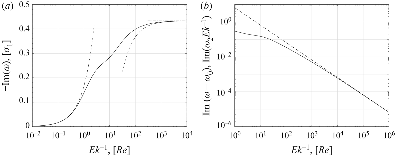
 $Ek\to 0$ the growth rates approach the inviscid growth rate, as may be anticipated (see Kubitschek & Weidman Reference Kubitschek and Weidman2007a, figure 3). The numerical calculation is repeated here, by way of verification of our results, and the imaginary part is shown (dashed) overlaying their solution (solid) in figure 9(a). The solutions are seen to coincide. The inviscid solution
 $-\textrm {Im}(\omega )=0.433$ is shown as the horizontal dot-dashed line and is given by solution of (2.31) in the viscous column limit with
 $R=1$,
 $m=0$ and
 $\delta _n=1$. In this special case, the eigenvalue
 $\omega$ is independent of the Weber number,
 $\textit {We}$. The asymptotic approximation in the high viscosity limit may be determined from the viscous column approximation to (B 1), (B 3), (B 7) and (B 8) and for
 $R=1$,
 $m=0$ and
 $\delta _n=1$ is given by
 \begin{equation} \omega\sim-\frac{I_1(1)^2\textrm{i}}{2I_0(1)^2 - 4I_1(1)^2}Ek^{-1} + O(Ek^{-2}) \approx -0.166\textrm{i}\,Ek^{-1}, \end{equation}
shown as the dashed curved line on the left-hand side of figure 9(a) that tends toward the numerical solutions as  $Ek\to \infty$,
 $Re\to 0$. For general
 $m$ and
 $\delta _n$ the approximation in the limit
 $Ek\to \infty$ is given in appendix C (C 1).
(a) The numerical solution for the imaginary part of  $\omega$ in the rotating viscous column reduced system with
 $\mathscr {A}=-1$,
 $\eta =-1$,
 $R=1$,
 $m=0$,
 $\delta _n=1$. In this limit the solution is independent of the Weber number,
 $\textit {We}$. The solution of Kubitschek & Weidman (Reference Kubitschek and Weidman2007a) figure 3 is shown solid and the present solution is shown dashed, overlaid and the two curves coincide. The inviscid solution due to (2.31) is the horizontal dashed line
 $\omega _0 \approx -0.433\textrm {i}$. The high viscosity asymptotic approximation is the dashed curve on the left, given by (4.3). The low viscosity asymptotic approximation is the dashed curve on the right, given by
 $\omega \approx \omega _0 + \omega _2Ek$, where
 $\omega _2$ is given by (4.4). (b) A comparison of the imaginary part of
 $\omega -\omega _0$ (solid) and the imaginary part of
 $\omega _2Ek$ (dashed). As the Ekman number increases it can be seen that the imaginary part of
 $\omega - \omega _0$ tends toward the imaginary part of
 $\omega _2Ek$ in agreement with the asymptotic expansion. (Quantities in square brackets use the notation of Kubitschek & Weidman (Reference Kubitschek and Weidman2007a).)

The correction to the inviscid growth rate in the low viscosity limit as calculated from § 2.3 is of the form  $\omega \sim \omega _0 + \omega _1Ek^{1/2} + O(Ek)$. However, in the special viscous column limit the coefficient
 $\omega _1$ is identically zero, and so if a higher-order approximation than the leading-order inviscid approximation is sought, a further term in the expansion is required. Following the same method as in § 2.3 taking the viscous column limit with
 $R=1$, the eigenvalue
 $\omega \sim \omega _0 + \omega _2Ek + O(Ek^{3/2})$ where
 $\omega _0$ is the inviscid eigenvalue given by (2.31) and the correction term is given in appendix C (C 2). In the special case considered in figure 9(a) for axisymmetric instability,
 $m=0$, and
 $\delta _n=1$ there is simplification and
 \begin{align} \omega_2 &= \frac{2\textrm{i}}{\omega_0^2 k_0}\left\{\left[\omega_0^4 - 8k_0^2 - 16\right] I_1(k_0)^2 - 2 k_0 \left[\omega_0^4 - 3\omega_0^2 + 4\right] I_0(k_0) I_1(k_0) + 8 k_0^2 I_0(k_0)^2\right\}\nonumber\\ &\quad \times\left\{k_0 \left(4 + [\omega_0^2 k_0]^2\right) I_0(k_0)^2 - \left[\left(4+ \omega_0^2\right) I_0(k_0) + 4 k_0 I_1(k_0)\right] I_1(k_0) \right\}^{-1}, \end{align}
where  $k_0$ is given by (2.23) and approximately
 $\omega \sim -0.433\textrm {i} + 6.63\textrm {i}\,Ek$. This approximation is shown as the curved dashed line on the right-hand side of figure 9(a) that coincides with the numerical solutions as
 $Ek\to 0$,
 $Re\to \infty$. The difference between the imaginary part of the full viscous eigenvalue,
 $\omega$, and the inviscid eigenvalue,
 $\omega _0$, is shown (solid line) in figure 9(b). The first term of the asymptotic approximation to this difference,
 $\omega _2Ek$, is shown dot-dashed and is in good agreement as
 $Ek\to 0$.
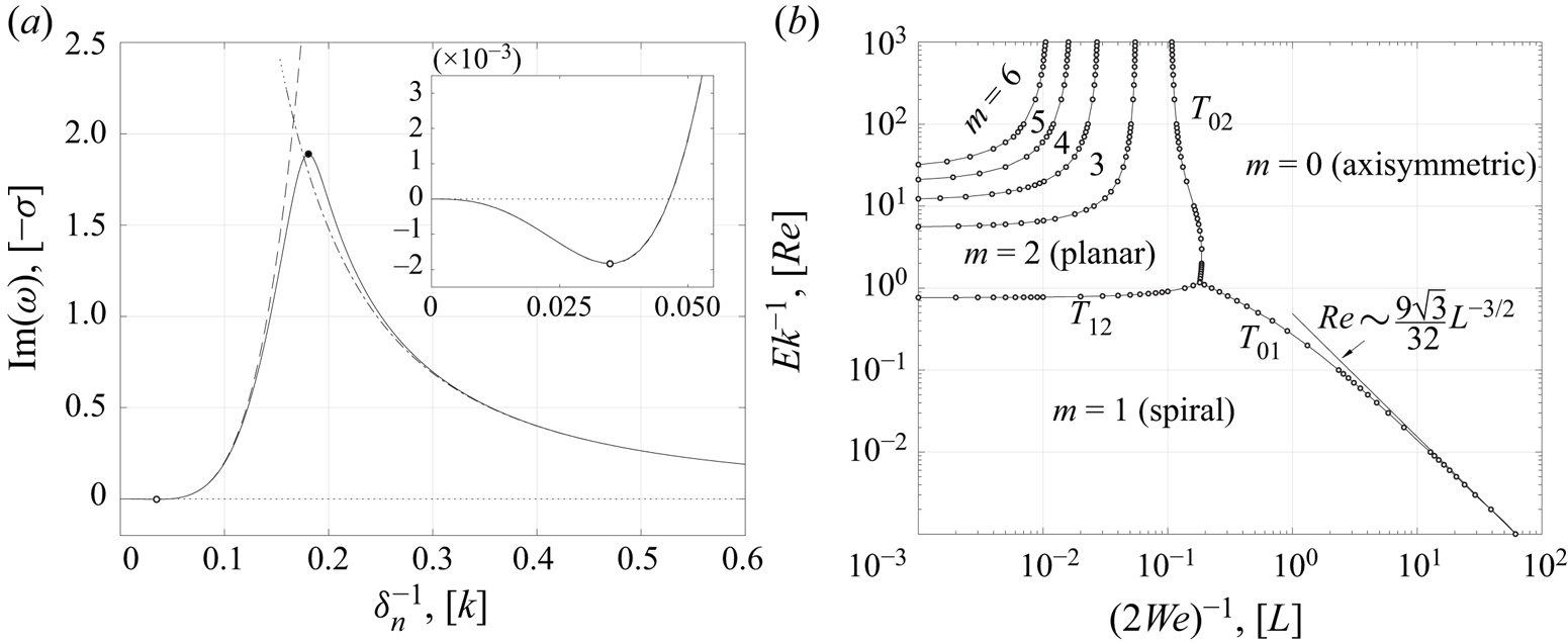
Kubitschek & Weidman (Reference Kubitschek and Weidman2007a) focused interest upon which of all the modes of instability has the highest growth rate for a given Ekman number and Weber number, as it might be anticipated that this dominant mode may be the observed mode of instability in a given realisation of the flow. The question of which mode is preferred, and the boundaries between these modes, were presented in their figure 13 (reproduced here in figure 10b). They note that in the high viscosity, high surface tension limit the two most unstable modes are the  $m=1$ ‘spiral’ mode instability and the
 $m=0$ axisymmetric mode instability. They further conjecture that the boundary between these two modes appears to follow asymptotic behaviour of the approximate form
 $Re\sim 0.5 L^{-3/2}$, in their notation.
(a) A numerical solution of the reduced system for  $Ek = 10^4$,
 $\textit {We} = (10^{-8/3})/2$,
 $m=1$. The high viscosity asymptotics of § 2.4, where
 $\textit {We}$ and
 $\delta _n$ are fixed, is shown dot-dashed. Scaling the Weber number as
 $Ek^{-2/3}$ and
 $\delta _n$ as
 $\delta _n\sim Ek^{1/3}$ leads to the approximation (4.5) which is shown dashed. The estimated most unstable mode is shown as the white data point. An enlargement of the approximation (dashed) in the neighbourhood of this turning point is compared with the numerics (solid) in the inset. The estimated most unstable mode is in good agreement with the full numerical solution. (b) The preferred mode diagram of Kubitschek & Weidman (Reference Kubitschek and Weidman2007a, figure 13) is reproduced with the asymptotic approximation to the
 $T_{01}$ boundary,
 $Re\sim 9\sqrt {3}/32\,L^{-3/2}$, indicated by the arrow. (Quantities in square brackets use the notation of Kubitschek & Weidman (Reference Kubitschek and Weidman2007a).)

A solution of the reduced system in this approximate region of parameter space is shown in figure 10(a) (solid line) for  $Ek = 10^4$,
 $L = 10^{8/3}$ (
 $=Ek^{2/3}$),
 $\alpha =1$,
 $m = 1$. The high viscosity asymptotics of § 2.4 for large Ekman number and fixed Weber number and
 $\delta _n$ is shown dot-dashed. The approximation is in good agreement in the region
 $\delta _n^{-1}\gtrsim 0.3$, but does not capture the behaviour of the full numerical solution for
 $\delta _n^{-1}\lesssim 0.2$. As
 $Ek$ is increased the turning point of the solution at
 $\delta _n^{-1}\approx 0.181$,
 $\textrm {Im}(\omega )\approx 1.89$ (indicated by the black circle) moves to the left, and the region in which the asymptotic approximation does not agree with the full numerical solution decreases. Indeed, as
 $Ek$ increases for any fixed
 $\delta _n$ and
 $\textit {We}$ the asymptotic approximation improves, as it must. However, the approximation does not capture the behaviour of the most unstable part of the solution if we treat the Weber number and
 $\delta _n$ as fixed parameters rather than coupling the Weber number and
 $\delta _n$ to the Ekman number. In order to capture the behaviour in the region
 $\delta _n^{-1}\lesssim 0.2$ we require a different asymptotic approximation to
 $\omega$, where
 $\textit {We}$ and
 $\delta _n$ are not fixed, but are proportional to powers of
 $Ek$.
In the region of  $(Re, L)$ space where
 $Re\sim L^{-3/2}$ we pose that the most unstable mode solutions to the reduced system in the
 $m=1$ spiral mode case behave as
 $\delta _n\sim Ek ^{1/3}$,
 $\textit {We}\sim Ek ^{-2/3}$, and
 $\omega \sim \omega _0^* +\omega _1^*Ek^{-1/3}+O(Ek^{-2/3})$, where
 $\omega _0^*$ is real and leads to precession of the mode only, rather than growth. (Equivalently in the notation of Kubitschek & Weidman (Reference Kubitschek and Weidman2007a),
 $k\sim Ek ^{-1/3}$,
 $L\sim Ek ^{2/3}$, which implies
 $k\sim Re ^{1/3}$,
 $L\sim Re ^{-2/3}$.) Here
 $\omega _0^*$ is distinct from the inviscid solution,
 $\omega _0$, given by (2.31). We seek solutions of the reduced system where
 $\textit {We} = \alpha ^2Ek^{-2/3}/2$,
 $\delta _n = K^{-1}Ek^{1/3}$ where
 $\alpha$ and
 $K$ are positive real constants of proportionality. We find in the
 $m=1$ spiral mode case that
 \begin{equation} \omega \sim 1 - \frac{K}{\alpha} + \frac{3\textrm{i}}{8}\left(K - \alpha\right)K^3Ek^{-1/3} + O\left(Ek^{-2/3}\right). \end{equation}
The growth rate of this spiral mode is  $O(Ek^{-1/3})$ and the most unstable mode is given by the stationary point at
 $K = 3\alpha /4$ where
 $\omega \sim 1/4 - (3\alpha )^4\textrm {i}2^{-11}Ek^{-1/3}$. The imaginary part of the approximation (4.5) is shown in figure 10(a) (dashed) and compares well with the full numerical solution (solid) in the region
 $\delta _n^{-1}\lesssim 0.2$. The estimate of the location and magnitude of the maximum growth rate given by
 $\min\{\textrm {Im}(\omega )\}$ is shown as the white circular data point. The neighbourhood of this turning point is shown enlarged in the inset where again the full numerical solution is shown as the solid line and the asymptotic approximation is shown dashed. The approximation is in excellent agreement with the numerical solution.
The equivalent result for the  $m=0$ axisymmetric mode is
 \begin{equation} \omega\sim-\frac{\textrm{i}}{6\alpha^2}Ek^{-1/3} + O\left(Ek^{-2/3}\right), \end{equation}
independent of  $K$. There is no precession of the axisymmetric mode, but the growth rate is
 $O(Ek^{-1/3})$, the same order of magnitude as the
 $m=1$ spiral mode. This therefore confirms the conjectured form of the
 $T_{01}$ boundary by Kubitschek & Weidman (Reference Kubitschek and Weidman2007a) and we are thus able to determine the value of
 $\alpha$ at which the preferred mode transitions from
 $m=0$ axisymmetric instability to
 $m=1$ spiral instability. The two growth rates are equal when
 \begin{equation} \frac{(3\alpha)^4}{2^{11}} = \frac{1}{6\alpha^2}, \end{equation}
balancing powers of  $Ek^{-1/3}$. The only positive real solution to (4.7) is
 $\alpha = (4/3)^{5/6}$, which gives the
 $T_{01}$ boundary as
 $Re\sim 9\sqrt {3}/32\,L^{-3/2}\approx 0.487 L^{-3/2}$ in the notation of Kubitschek & Weidman (Reference Kubitschek and Weidman2007a), in good agreement with their numerical estimate.
The straightforward forms of (4.5) and (4.6) do not reflect the manipulations required to determine them. Asymptotic approximations to the coefficients  $b_{1j}$ are required, and these series begin at
 $O(Ek^{1/3})$ and descend in powers of
 $Ek^{1/9}$. Sufficient terms to determine
 $b_{1j}$ at
 $O(Ek^{-5/9})$ are required for the solution to be determined. Similarly the required solution to (2.9) is a series that begins at
 $O(Ek^{-1/3})$ and also descends in powers of
 $Ek^{1/9}$ and must be expanded to
 $O(Ek^{-11/9})$ in order to determine
 $\omega _0^*$ and
 $\omega _1^*$.
5. Discussion and conclusions
We have investigated the three-dimensional centrifugally driven Rayleigh–Taylor instability, in particular the very high rotational limit of the rotating Rayleigh–Taylor instability in which the effects of gravity may be neglected. A cylindrical domain and initially cylindrical interface between the two fluid layers have been modelled. We have considered the inviscid case, the low viscosity case and the high viscosity case. In all three cases the system is subject to linear instability when the inner layer is denser than the outer layer or, equivalently, the Atwood number, as we have defined it, is negative.
We defined a non-dimensional Ekman number in terms of the mean viscosity, mean density, rotation rate and domain radius such that the low viscosity regime is characterised by a small Ekman number and the high viscosity regime is characterised by a typically large Ekman number. The growth and precession rates in the low viscosity regime are an  $O(Ek^{1/2})$ correction to the inviscid growth and precession rate. The growth rate in the high viscosity regime is
 $O(Ek^{-1})$ while the precession rate is
 $O(Ek^{-2})$.
In the stable configuration ( $\mathscr {A}>0$) a similar asymptotic dependence on the Ekman number is observed. In the low viscosity limit the oscillation rate and precession rate behave as an
 $O(Ek^{1/2})$ correction to the inviscid oscillation and precession rate. In the high viscosity limit the oscillation and precession rate behave as
 $O(Ek^{-1})$.
In the unstable high viscosity limit the growth rate behaves as  $O(Ek^{-1})$ and in the special case that surface tension may be neglected has a linear dependence on the Atwood number. This means that the preferred mode of instability in this limit is independent of the absolute values of the viscosity and independent of the density in each layer; the preferred mode in this limit is determined only by the aspect ratio of the domain,
 $\delta$, the non-dimensional viscosity contrast,
 $\eta$ and the initial location of the unperturbed interface,
 $R$.
Finally, we showed how our results apply to the special limiting case of a rotating viscous column of fluid in the absence of gravity. For fixed wavenumber and Weber number our asymptotics describe the growth rate of perturbations to the rotating viscous column when the density and viscosity of the outer fluid layer a taken to be zero. In contrast to the general two-layer arrangement, in this special single fluid layer case, in the low viscosity limit, there is an  $O(Ek)$ correction to the inviscid growth rate. The boundary over which the preferred mode of growth changes from varicose to spiral in a high viscosity, high surface tension regime is shown to behave as
 $Ek\sim 2^{7/2}3^{-5/2}\textit {We}^{-3/2}\approx 0.726\textit {We}^{-3/2}$.
Our results follow from a linear stability analysis and so are subject to the usual caveats. We cannot draw conclusions relating to any subcritical instability or nonlinear interactions between the various possible modes of instability.
Acknowledgements
The authors would like to acknowledge the financial support of the Woods Hole GFD Summer Program 2018, where this research was initiated. We would also like to thank an anonymous referee for encouraging us to compare our results with those of Kubitschek & Weidman (Reference Kubitschek and Weidman2007a).
Declaration of interests
The authors report no conflict of interest.
Appendix A. Low viscosity asymptotic system
The coefficients  $\hat {b}_{ij}$,
 $\hat {c}_{2j}$ for
 $i=1,2$,
 $j=2,3$ are shown here for completeness, but their values do not need to be explicitly determined if only the growth rate correction,
 $\omega _1$, is required;
 \begin{align} \hat{b}_{12} &= - \frac{\textrm{e}^{\textrm{i} R/(\omega_0 \delta_n)}}{8} \exp\left\{ - \textrm{e}^{\textrm{i} {\rm \pi}/4}\frac{\sqrt{1 - \mathscr{A}}}{\sqrt{1 - \eta}}\frac{R \omega_1}{2\omega_0^{1/2}}\right\} \left\{R \left[1 + \left(\frac{1 - \mathscr{A}}{1 + \mathscr{A}}\right)^{1/2}\left(\frac{1 - \eta}{1 + \eta}\right)^{1/2}\right]\right\}^{-1}\nonumber\\ &\quad \times \left\{ - 2\textrm{i} \left[ c_{210} K_{m + 1}(k_0 R) + I_{m + 1}(k_0 R) \left(b_{110} - b_{210} \right) \right] \delta_n k_0 \omega_0 R \right. \nonumber\\ &\quad \left. +\left[\left(\textrm{i} \delta_n m + R \right) \omega_0 - 2 R\right] \left[( b_{210} - b_{110}) I_m(k_0 R) + c_{210} K_m(k_0 R)\right] (\omega_0 + 2)\vphantom{\left\{ - 2\textrm{i} \left[ c_{210} K_{m + 1}(k_0 R) + I_{m + 1}(k_0 R) \left(b_{110} - b_{210} \right) \right] \delta_n k_0 \omega_0 R \right.}\right\} \end{align}
 \begin{align} \hat{b}_{13} &= \frac{\textrm{e}^{-\textrm{i} R/(\omega_0 \delta_n)}}{8} \exp\left\{ - \textrm{e}^{\textrm{i} {\rm \pi}/4}\frac{\sqrt{1 - \mathscr{A}}}{\sqrt{1 - \eta}}\frac{R \omega_1}{2\omega_0^{1/2}}\right\} \left\{R \left[1 + \left(\frac{1 - \mathscr{A}}{1 + \mathscr{A}}\right)^{1/2}\left(\frac{1 - \eta}{1 + \eta}\right)^{1/2}\right]\right\}^{-1}\nonumber\\ &\quad \times \left\{ - 2\textrm{i} \left[c_{210} K_{m + 1}(k_0 R) + I_{m + 1}(k_0 R) \left(b_{110} - b_{210} \right)\right] \delta_n k_0 \omega_0 R \right. \nonumber\\ &\quad \left. +\left[\left(\textrm{i} \delta_n m - R \right) \omega_0 + 2 R \right] \left[( - b_{110} + b_{210}) I_m(k_0 R) + c_{210} K_m(k_0 R)\right] (\omega_0 + 2) \vphantom{\left\{ - 2\textrm{i} \left[ c_{210} K_{m + 1}(k_0 R) + I_{m + 1}(k_0 R) \left(b_{110} - b_{210} \right) \right] \delta_n k_0 \omega_0 R \right.}\right\} \end{align}
 \begin{align} \hat{b}_{22} &= \frac{\textrm{e}^{\textrm{i}/(\omega_0 \delta_n)}}{8} \exp\left\{ - \textrm{e}^{\textrm{i} {\rm \pi}/4}\frac{\sqrt{1 + \mathscr{A}}}{\sqrt{1 + \eta}}\frac{\omega_1}{2\omega_0^{1/2}}\right\}\nonumber\\ &\quad \times \left\{ 2\textrm{i} \omega_0 k_0 \delta_n \left(b_{210} I_{m + 1}(k_0) - c_{210} K_{m + 1}(k_0)\right) \right. \nonumber\\ &\quad \left. + (\omega_0 + 2)(\textrm{i} m \omega_0 \delta_n + \omega_0 - 2) (I_m(k_0) b_{210} + K_m(k_0) c_{210})\vphantom{\left\{ - 2\textrm{i} \left[ c_{210} K_{m + 1}(k_0 R) + I_{m + 1}(k_0 R) \left(b_{110} - b_{210} \right) \right] \delta_n k_0 \omega_0 R \right.}\right\} \end{align}
 \begin{align} \hat{b}_{23} &= - \frac{\textrm{e}^{-\textrm{i}/(\omega_0 \delta_n)}}{8} \exp\left\{ - \textrm{e}^{\textrm{i} {\rm \pi}/4}\frac{\sqrt{1 + \mathscr{A}}}{\sqrt{1 + \eta}}\frac{\omega_1}{2\omega_0^{1/2}}\right\}\nonumber\\ &\quad \times \left\{ 2\textrm{i} \omega_0 k_0 \delta_n \left(b_{210} I_{m + 1}(k_0) - c_{210} K_{m + 1}(k_0) \right) \right. \nonumber\\ &\quad \left. + (\omega_0 + 2) (\textrm{i} m \omega_0 \delta_n - \omega_0 + 2) (I_m(k_0) b_{210} + K_m(k_0) c_{210})\vphantom{\left\{ - 2\textrm{i} \left[ c_{210} K_{m + 1}(k_0 R) + I_{m + 1}(k_0 R) \left(b_{110} - b_{210} \right) \right] \delta_n k_0 \omega_0 R \right.}\right\} \end{align}
 \begin{align} \hat{c}_{22} &= - \frac{ \textrm{e}^{-\textrm{i} R/(\omega_0 \delta_n)}}{8} \exp\left\{\textrm{e}^{\textrm{i} {\rm \pi}/4}\frac{\sqrt{1 + \mathscr{A}}}{\sqrt{1 + \eta}}\frac{R \omega_1}{2\omega_0^{1/2}}\right\} \left\{R \left[1 + \left(\frac{1 + \mathscr{A}}{1 - \mathscr{A}}\right)^{1/2}\left(\frac{1 + \eta}{1 - \eta}\right)^{1/2}\right]\right\}^{-1}\nonumber\\ &\quad \times \left\{ - 2\textrm{i} \left[ c_{210} K_{m + 1}(k_0 R) + I_{m + 1}(k_0 R) \left(b_{110} - b_{210} \right)\right] \delta_n k_0 \omega_0 R \right. \nonumber\\ &\quad \left. + \left[\left(\textrm{i} \delta_n m - R \right) \omega_0 + 2 R \right] \left[( b_{210} - b_{110}) I_m(k_0 R) + c_{210} K_m(k_0 R)\right] (\omega_0 + 2)\vphantom{\left\{ - 2\textrm{i} \left[ c_{210} K_{m + 1}(k_0 R) + I_{m + 1}(k_0 R) \left(b_{110} - b_{210} \right) \right] \delta_n k_0 \omega_0 R \right.}\right\} \end{align}
 \begin{align} \hat{c}_{23}& = \frac{\textrm{e}^{\textrm{i} R/(\omega_0 \delta_n)}}{8} \exp\left\{\textrm{e}^{\textrm{i} {\rm \pi}/4}\frac{\sqrt{1 + \mathscr{A}}}{\sqrt{1 + \eta}}\frac{R \omega_1}{2\omega_0^{1/2}}\right\} \left\{R \left[1 + \left(\frac{1 + \mathscr{A}}{1 - \mathscr{A}}\right)^{1/2}\left(\frac{1 + \eta}{1 - \eta}\right)^{1/2}\right]\right\}^{-1}\nonumber\\ &\quad \times \left\{ - 2\textrm{i} \left[ c_{210} K_{m + 1}(k_0 R) + I_{m + 1}(k_0 R) \left(b_{110} - b_{210} \right) \right] \delta_n k_0 \omega_0 R \right. \nonumber\\ &\quad \left. + \left[\left(\textrm{i} \delta_n m + R \right) \omega_0 - 2 R \right] \left[( b_{210} - b_{110} ) I_m(k_0 R) + c_{210} K_m(k_0 R)\right] (\omega_0 + 2). \vphantom{\left\{ - 2\textrm{i} \left[ c_{210} K_{m + 1}(k_0 R) + I_{m + 1}(k_0 R) \left(b_{110} - b_{210} \right) \right] \delta_n k_0 \omega_0 R \right.}\right\} \end{align}
Appendix B. High viscosity asymptotic system
The universal boundary and matching conditions are given by: the kinematic condition for the inner layer,
 \begin{align} &\left[\left(m^2 \delta_n^2 + R^2\right)\alpha_{11} -\textrm{i} m \delta_n^2 \left(\frac{2}{\delta_n}\right)^{2/3} \left(\frac{1-\eta}{1-\mathscr{A}}\right)^{1/3} \lambda_2 \beta_{11}\right] I_m\left(\frac{R}{\delta_n}\right)\nonumber\\ &\quad + \lambda_2 \left(\frac{2}{\delta_n}\right)^{1/3}\left(\frac{1-\eta}{1-\mathscr{A}}\right)^{2/3}\left[ m \delta_n I_m\left(\frac{R}{\delta_n}\right) + R I_{m+1}\left(\frac{R}{\delta_n}\right)\right] \gamma_{11} = \frac{2 \textrm{i} R \delta_n^2}{3} \omega_0; \end{align}
the kinematic condition for the outer layer,
 \begin{align} &-\textrm{i} m \lambda_2\delta_n^2 \left(\frac{2}{\delta_n}\right)^{2/3} \left(\frac{1+\eta}{1+\mathscr{A}}\right)^{1/3}\left[I_m\left(\frac{R}{\delta_n}\right) \beta_{21} + K_m\left(\frac{R}{\delta_n}\right) \beta_{22}\right]\nonumber\\ &\qquad +\lambda_2 \left(\frac{2}{\delta_n}\right)^{1/3} \left(\frac{1+\eta}{1+\mathscr{A}}\right)^{2/3} \left\{\left[m \delta_n I_m\left(\frac{R}{\delta_n}\right)+ R I_{m+1}\left(\frac{R}{\delta_n}\right)\right] \gamma_{21} \right. \nonumber\\ &\qquad \left. + \left[ m \delta_n K_m\left(\frac{R}{\delta_n}\right) - R K_{m+1}\left(\frac{R}{\delta_n}\right)\right] \gamma_{22}\right\}\nonumber\\ &\qquad +\left[m^2 \delta_n^2 I_m\left(\frac{R}{\delta_n}\right)+ R^2 I_m\left(\frac{R}{\delta_n}\right)\right] \alpha_{21} + \left[m^2 \delta_n^2 K_m\left(\frac{R}{\delta_n}\right)+R^2 K_m\left(\frac{R}{\delta_n}\right)\right] \alpha_{22} \nonumber\\ &\quad = \frac{2\textrm{i} R \delta_n^2}{3}\omega_0; \end{align}
the normal (radial) stress continuity condition,
 \begin{align} &\frac{2}{\delta_n}\left[\left((m-1) m \delta_n^2+R^2\right) m \delta_n I_m\left(\frac{R}{\delta_n}\right) + \left(m^2 \delta_n^2 + R^2\right)R I_{m+1}\left(\frac{R}{\delta_n}\right)\right]\nonumber\\ &\quad \times \left[\left(1-\eta\right) \alpha_{11} - \left(1 + \eta\right) \alpha_{21}\right] -\frac{2}{\delta_n}\left[\left((m-1)m \delta_n^2+R^2\right) m \delta_n K_m\left(\frac{R}{\delta_n}\right) \right.\nonumber\\ &\quad \left.- \left(m^2 \delta_n^2 + R^2\right)R K_{m+1}\left(\frac{R}{\delta_n}\right) \right]\left(1+\eta\right) \alpha_{22}-\textrm{i} \lambda_2 m \delta_n^2 \left(\frac{2}{\delta_n}\right)^{5/3}\nonumber\\ &\quad\times \left\{\left[(m-1) \delta_n I_m\left(\frac{R}{\delta_n}\right) + R I_{m+1}\left(\frac{R}{\delta_n}\right)\right] \left[\frac{(1-\eta)^{4/3}}{(1-\mathscr{A})^{1/3}}\beta_{11} - \frac{(1+\eta)^{4/3}}{(1+\mathscr{A})^{1/3}} \beta_{21}\right] \right. \nonumber\\ &\quad \left. -\left[(m-1) \delta_n K_m\left(\frac{R}{\delta_n}\right) - R K_{m+1}\left(\frac{R}{\delta_n}\right)\right] \frac{(1+\eta)^{4/3}}{(1+\mathscr{A})^{1/3}} \beta_{22}\right\}\nonumber\\ &\quad +\lambda_2\left(\frac{2}{\delta_n}\right)^{4/3}\left\{ \left[\left((m-1)m\delta_n^2+R^2\right)I_m\left(\frac{R}{\delta_n}\right)-R\delta_n I_{m+1}\left(\frac{R}{\delta_n}\right)\right]\right.\nonumber\\ &\quad\times\left[\frac{(1-\eta)^{5/3}}{(1 - \mathscr{A})^{2/3}} \gamma_{11} - \frac{(1+\eta)^{5/3}}{(1+\mathscr{A})^{2/3}} \gamma_{21}\right] \nonumber\\ &\quad \left. - \left[\left((m-1)m \delta_n^2+R^2\right)K_m\left(\frac{R}{\delta_n}\right)+ R\delta_nK_{m+1}\left(\frac{R}{\delta_n}\right)\right] \frac{(1+\eta)^{5/3}}{(1+\mathscr{A})^{2/3}} \gamma_{22}\right\}\nonumber\\ &\qquad = -\frac{4\delta_n^2 R^3 \mathscr{A}}{3} - \frac{2}{3\,\textit{We}}\left[\left(m^2 - 1\right)\delta_n^2+R^2\right], \end{align}
(the final term in the right-hand side of (B 3) is the only surface tension term in the whole system (B 1)–(B 10)); the final universal condition is the no-penetration condition on  $r=1$,
 \begin{align} &-\textrm{i} m \delta_n^2\left(\frac{2}{\delta_n}\right)^{2/3} \left(\frac{1+\eta}{1+\mathscr{A}}\right)^{1/3}\left[I_m\left(\frac{1}{\delta_n}\right) \beta_{21} + K_m\left(\frac{1}{\delta_n}\right) \beta_{22}\right] \nonumber\\ &\quad +\lambda_1\left(1 + m^2\delta_n^2\right)\left[I_m\left(\frac{1}{\delta_n}\right) \alpha_{21} + K_m\left(\frac{1}{\delta_n}\right) \alpha_{22}\right] +\left(\frac{2}{\delta_n}\right)^{1/3}\left(\frac{1+\eta}{1+\mathscr{A}}\right)^{2/3} \nonumber\\ &\quad \times \left\{\left[m \delta_n I_m\left(\frac{1}{\delta_n}\right) + I_{m+1}\left(\frac{1}{\delta_n}\right)\right] \gamma_{21} + \left[m \delta_n K_m\left(\frac{1}{\delta_n}\right)-K_{m+1}\left(\frac{1}{\delta_n}\right)\right] \gamma_{22}\right\} =0. \end{align}
The viscous boundary and matching conditions are given by: the azimuthal velocity continuity condition,
 \begin{align} &\left[m \delta_n I_m\left(\frac{R}{\delta_n}\right) + R I_{m+1}\left(\frac{R}{\delta_n}\right)\right] \nonumber\\ &\quad \times \left\{\textrm{i} m \left(\alpha_{11} - \alpha_{21}\right)+ \lambda_2 \left(\frac{2}{\delta_n}\right)^{2/3}\left[\left(\frac{1-\eta}{1-\mathscr{A}}\right)^{1/3} \beta_{11} - \left(\frac{1+\eta}{1+\mathscr{A}}\right)^{1/3} \beta_{21}\right]\right\}\nonumber\\ &\quad -\left[m \delta_n K_m\left(\frac{R}{\delta_n}\right) - R K_{m+1}\left(\frac{R}{\delta_n}\right)\right]\left[\textrm{i} m \alpha_{22} + \lambda_2\left(\frac{2}{\delta_n}\right)^{2/3}\left(\frac{1+\eta}{1+\mathscr{A}}\right)^{1/3} \beta_{22} \right]\nonumber\\ &\quad +\textrm{i} m \lambda_2 \left(\frac{2}{\delta_n}\right)^{1/3} \left\{\left(\frac{1-\eta}{1-\mathscr{A}}\right)^{2/3} I_m\left(\frac{R}{\delta_n}\right) \gamma_{11} \right. \nonumber\\ &\quad \left. -\left(\frac{1+\eta}{1+\mathscr{A}}\right)^{2/3}\left[ I_m\left(\frac{R}{\delta_n}\right) \gamma_{21} + K_m\left(\frac{R}{\delta_n}\right) \gamma_{22}\right]\right\}=0; \end{align}
the axial velocity continuity condition,
 \begin{align} &\left[(m+2) \delta_n I_m\left(\frac{R}{\delta_n}\right) + R I_{m+1}\left(\frac{R}{\delta_n}\right)\right] \left(\alpha_{11} - \alpha_{21}\right)\nonumber\\ &\quad -\left[(m+2) \delta_n K_m\left(\frac{R}{\delta_n}\right) - R K_{m+1}\left(\frac{R}{\delta_n}\right)\right] \alpha_{22} +\lambda_2 \left(\frac{2}{\delta_n}\right)^{1/3}\left\{ \left(\frac{1-\eta}{1 - \mathscr{A}}\right)^{2/3}I_m\left(\frac{R}{\delta_n}\right)\gamma_{11} \right. \nonumber\\ &\quad \left. - \left(\frac{1+\eta}{1+\mathscr{A}}\right)^{2/3}\left[I_m\left(\frac{R}{\delta_n}\right) \gamma_{21} + K_m\left(\frac{R}{\delta_n}\right) \gamma_{22}\right]\right\} = 0; \end{align}
the azimuthal stress continuity condition,
 \begin{align} &\textrm{i} m \lambda_1 \left\{ \left[\left((m-1) m \delta_n^2 + R^2\right) I_m\left(\frac{R}{\delta_n}\right) - R \delta_n I_{m+1}\left(\frac{R}{\delta_n}\right)\right] \left[(1+\eta)\alpha_{21} - (1-\eta) \alpha_{11}\right] \right. \nonumber\\ &\quad \left. +\left[\left((m-1) m \delta_n^2 + R^2\right) K_m\left(\frac{R}{\delta_n}\right) + R \delta_nK_{m+1}\left(\frac{R}{\delta_n}\right)\right](1+\eta) \alpha_{22}\right\}\nonumber\\ &\quad -\left(\frac{2}{\delta_n}\right)^{2/3}\left\{ \left[\left((m-1) m \delta_n^2+\frac{R^2}{2}\right)I_m\left(\frac{R}{\delta_n}\right) \right.\right.\nonumber\\ &\quad \left.\left.- R \delta_n I_{m+1}\left(\frac{R}{\delta_n}\right)\right] \left[\frac{(1-\eta)^{4/3}}{(1-\mathscr{A})^{1/3}} \beta_{11} - \frac{(1+\eta)^{4/3}}{(1+\mathscr{A})^{1/3}} \beta_{21}\right] \right. \nonumber\\ &\quad \left. -\left[\left((m-1) m \delta_n^2 + \frac{R^2}{2}\right)K_m\left(\frac{R}{\delta_n}\right) + R \delta_n K_{m+1}\left(\frac{R}{\delta_n}\right)\right] \frac{(1+\eta)^{4/3}}{(1+\mathscr{A})^{1/3}} \beta_{22}\right\}\nonumber\\ &\quad -\textrm{i} \left(\frac{2}{\delta_n}\right)^{1/3}m \left\{ \left[(m-1) \delta_n I_m\left(\frac{R}{\delta_n}\right)+ R I_{m+1}\left(\frac{R}{\delta_n}\right)\right]\right.\nonumber\\ &\quad \times \left[\frac{(1-\eta)^{5/3}}{(1-\mathscr{A})^{2/3}} \gamma_{11} - \frac{(1+\eta)^{5/3}}{(1+\mathscr{A})^{2/3}} \gamma_{21}\right] \nonumber\\ &\quad \left. -\left[(m-1) \delta_n K_m\left(\frac{R}{\delta_n}\right) -R K_{m+1}\left(\frac{R}{\delta_n}\right)\right] \frac{(1+\eta)^{5/3}}{(1+\mathscr{A})^{2/3}} \gamma_{22}\right\}=0; \end{align}
the axial stress continuity condition,
 \begin{align} &\frac{2}{\delta_n}\left[\left((m+1) m \delta_n^2+R^2\right)I_m\left(\frac{R}{\delta_n}\right) + R \delta_n I_{m+1}\left(\frac{R}{\delta_n}\right)\right] \left[(1-\eta) \alpha_{11} - (1+\eta) \alpha_{21}\right]\nonumber\\ &\quad-\frac{2}{\delta_n}\left[\left((m+1) m \delta_n^2 + R^2\right) K_m\left(\frac{R}{\delta_n}\right) - R \delta_n K_{m+1}\left(\frac{R}{\delta_n}\right)\right](1+\eta) \alpha_{22}\nonumber\\ &\quad -\textrm{i} \lambda_2 \left(\frac{2}{\delta_n}\right)^{2/3} m \delta_n \left\{I_m\left(\frac{R}{\delta_n}\right)\left[\frac{(1-\eta)^{4/3}}{(1-\mathscr{A})^{1/3}} \beta_{11}- \frac{(1+\eta)^{4/3}}{(1+\mathscr{A})^{1/3}} \beta_{21}\right]\right.\nonumber\\ &\quad \left.-K_m\left(\frac{R}{\delta_n}\right)\frac{(1+\eta)^{4/3}}{(1+\mathscr{A})^{1/3}} \beta_{22}\right\}\nonumber\\ &\quad +\lambda_2\left(\frac{2}{\delta_n}\right)^{4/3}\left\{ \left[m \delta_n I_m\left(\frac{R}{\delta_n}\right) + R I_{m+1}\left(\frac{R}{\delta_n}\right)\right] \left[\frac{(1-\eta)^{5/3}}{(1-\mathscr{A})^{2/3}} \gamma_{11} -\frac{(1+\eta)^{5/3}}{(1+\mathscr{A})^{2/3}} \gamma_{21}\right] \right.\nonumber\\ &\quad \left. -\left[m \delta_n K_m\left(\frac{R}{\delta_n}\right) - R K_{m+1}\left(\frac{R}{\delta_n}\right)\right] \frac{(1+\eta)^{5/3}}{(1+\mathscr{A})^{2/3}} \gamma_{22}\right\}=0; \end{align}
the azimuthal no-slip condition,
 \begin{align} &\left[m \delta_n I_m\left(\frac{1}{\delta_n}\right) + I_{m+1}\left(\frac{1}{\delta_n}\right)\right] \left[m\lambda_1\alpha_{21} -\textrm{i}\left(\frac{2}{\delta_n}\right)^{2/3}\left(\frac{1+\eta}{1 + \mathscr{A}}\right)^{1/3}\beta_{21}\right]\nonumber\\ &\quad + \left[m \delta_n K_m\left(\frac{1}{\delta_n}\right)-K_{m+1}\left(\frac{1}{\delta_n}\right)\right] \left[m\lambda_1\alpha_{22} -\textrm{i}\left(\frac{2}{\delta_n}\right)^{2/3}\left(\frac{1+\eta}{1 + \mathscr{A}}\right)^{1/3}\beta_{22}\right]\nonumber\\ &\quad +m\left(\frac{2}{\delta_n}\right)^{1/3}\left(\frac{1+\eta}{1+\mathscr{A}}\right)^{2/3} \left[I_m\left(\frac{1}{\delta_n}\right) \gamma_{21}+K_m\left(\frac{1}{\delta_n}\right) \gamma_{22}\right] = 0; \end{align}
and finally the axial no-slip condition,
 \begin{align} &\left[(m+2)\delta_n I_m\left(\frac{1}{\delta_n}\right) + I_{m+1}\left(\frac{1}{\delta_n}\right)\right]\alpha_{21} +\left[(m+2)\delta_nK_m\left(\frac{1}{\delta_n}\right)-K_{m+1}\left(\frac{1}{\delta_n}\right)\right] \alpha_{22}\nonumber\\ &\quad +\left(\frac{2}{\delta_n}\right)^{1/3}\left(\frac{1+\eta}{1+\mathscr{A}}\right)^{2/3}\lambda_2 \left[K_m\left(\frac{1}{\delta_n}\right) \gamma_{22} + I_m\left(\frac{1}{\delta_n}\right)\gamma_{21}\right] = 0. \end{align}
Appendix C. Rotating viscous column system
In (4.3) the high viscosity approximation for the rotating viscous column in the axisymmetric case  $m=0$, with
 $\delta _n=1$ was given. It is a special case of the general approximation,
 \begin{align} \omega &\sim \frac{\textrm{i}Ek^{-1}}{4\textit{We}} \left\{2\delta_n I_{m+1}^3(\delta_n^{-1}) +\left[(m+6)m\delta_n^2-1\right] I_m(\delta_n^{-1}) I_{m+1}(\delta_n^{-1})^2\right. \nonumber\\ &\quad \left. +2\left[(m+2)m\delta_n^2-1\right] m \delta_n I_m^2(\delta_n^{-1}) I_{m+1}(\delta_n^{-1}) - 2m^2 \delta_n^2 I_m^3(\delta_n^{-1}) \right\}\nonumber\\ &\quad \times \left[(m^2-2\textit{We}-1)\delta_n^2+1\right]\left\{ \left[1+m(m^3 + 6 m^2 - m - 6) \delta_n^4 \right.\right.\nonumber\\ &\quad \left.+(2m^2 - 6m + 1)\delta_n^2 \right] I_m(\delta_n^{-1}) I_{m+1}^2(\delta_n^{-1}) +2\delta_n\left[ (m^3+2m^2-m-2) m^2 \delta_n^4\right.\nonumber\\ &\quad \left.+(2m^2-3m+1)m\delta_n^2+m+1\right] I_m^2(\delta_n^{-1}) I_{m+1}(\delta_n^{-1})\nonumber\\ &\quad +2\delta_n\left[(m^2-1)\delta_n^2 - 1\right] I_{m+1}^3(\delta_n^{-1})\nonumber\\ &\quad \left.-\left[1+(m^2+2m-3)m^2\delta_n^4+2(m-1)m\delta_n^2\right] I_m^3(\delta_n^{-1})\right\}^{-1}. \end{align}
This expression is determined by taking the viscous column approximation,  $\mathscr {A}=-1$,
 $\eta =-1$, to (B 1), (B 3), (B 7) and (B 8), and setting
 $R=1$.
In (4.4) the low viscosity approximation for the rotating viscous column in the axisymmetric case  $m=0$, with
 $\delta _n=1$ was given. The general approximation for arbitrary
 $m$ and
 $\delta _n$ is given by
 \begin{align} \omega_2 &= \frac{2\textrm{i}}{\delta_n^2\omega_0^2} \left[(m^2 - 2\textit{We} - 1)\delta_n^2 + 1\right]\left\{(\omega_0^2 -4)\left[8 + \omega_0^2 (4m\omega_0 - \omega_0^2 - 4)\delta_n^2\right] I_{m+1}(k_0)^2\right.\nonumber\\ &\quad + 2\left[m\omega_0^2(\omega_0 + 2)^2(m - 1)\delta_n^2 + \omega_0^4 - 3\omega_0^2 + 4(2m + 1)\right] k_0\delta_n^2\omega_0^2I_m(k_0)I_{m+1}(k_0)\nonumber\\ &\quad + 2(\omega_0 + 2)\left[m^2\omega_0^4(\omega_0 + 2)(m - 1)\delta_n^4\right.\nonumber\\ &\quad +\left.\left. m\omega_0^2(\omega_0 + 2)(\omega_0 - 1)^2\delta_n^2 - 4(\omega_0 -2)\right]I_m(k_0)^2\right\}\nonumber\\ &\quad \times\left\{ \left[(m^2 - 2\textit{We} - 1)\delta_n^2 + 1\right]\left[4k_0 I_{m+1}(k_0) + (\omega_0^2 + 8m + 4)I_m(k_0) \right]k_0\delta_n^2\omega_0^2I_{m+1}(k_0)\right.\nonumber\\ &\quad + (\omega_0 + 2)\left[(\omega_0 + 2)\left(2\left[\left(\omega_0 - 2\right)^2 - m\right]\textit{We} + m\left(m^2-1\right)\right)\delta_n^4\omega_0^2\right.\nonumber\\ &\quad \left.\left.+ \left[m\omega_0^2\left(\omega_0+2\right) - 4(m^2 -2\textit{We} -1)(\omega_0 -2)\right]\delta_n^2 - 4(\omega_0 -2)\right]I_m(k_0)^2\right\}^{-1}. \end{align}