


I. INTRODUCTION
In X-ray crystallography, the structure of a crystal is actually the electron density distribution in the crystal. The electron density distribution of a crystal is the inverse Fourier transform of its structure factors. Unfortunately, only structure amplitudes can be derived from the experimentally recorded diffraction intensity data; phases of the structure factors usually cannot be measured directly. Various techniques have been developed to derive the phases and then build the electron density map, such as the direct methods (Karle and Hauptman, Reference Karle and Hauptman1950; Woolfson, Reference Woolfson1987; Woolfson and Fan, Reference Woolfson and Fan1995), which have been dominating the small-molecule X-ray crystallography. In a previous paper (Li et al., Reference Li, He and Zhang2015), we have proposed a new strategy to derive the phases for observed structure amplitudes: the correctly retrieved electron density map is identified by an evaluation function (or a figure of merit) from a tremendous number of electron density models, which are constructed by assigning all possible phase sets (within certain accuracy) to the observed structure amplitudes. Two evaluation functions were proposed for this purpose. Recently, Burla et al. (Reference Burla, Carrozzini, Cascarano, Giacovazzo and Polidori2017) developed a multipurpose figure of merit, MPF, which can also be used in recognizing the quality of a current electron density model. Here, we put forward another evaluation function (or figure of merit) for identifying the correct electron density map. Instead of examining the electron density model itself, this evaluation function assesses the agreement between the calculated and expected structure amplitudes of the modified electron density model.
Indeed, iterative electron density modification methods for structure determination, such as the charge flipping methods (Oszlányi and Sütő, Reference Oszlányi and Sütő2004, Reference Oszlányi and Sütő2008), have been developed a long time ago, and are gaining their popularity. In the process of structure determination using the iterative electron density modification method, the initial electron density model is usually obtained by the inverse Fourier synthesis using observed structure amplitudes and random phases. The obtained electron density map is modified in a particular way in each following iterative cycle, and the correct electron density map may be obtained finally. Oszlányi and Sütő have proposed an R factor to monitor the convergence of charge flipping iterations (Oszlányi and Sütő, Reference Oszlányi and Sütő2004). This R factor measures how well the calculated structure amplitudes of the modified current electron density model agree with the observed ones. Inspired by the R factor proposed by Oszlányi and Sütő, we conceived an evaluation function, which hopefully can be used to identify the correct electron density model. The details of this evaluation function will be presented in the following sections.
II. DEFINITION AND CALCULATION
A. Notation
-
EDM: electron density modification.
-
FT: Fourier transform.
-
IFT: inverse Fourier transform.
-
ρ cryst: the electron density distribution in a real crystal.
-
ρ o: the image of ρ cryst at a certain resolution, which is calculated by IFT using the observed structure amplitudes and correct phases.
-
ρ: the current electron density model which is calculated by IFT using the observed structure amplitudes and the current trial phase set.
-
ρ o*: the resultant electron density map after ρ o has been modified in a particular way.
-
ρ*: the resultant electron density map after the current electron density model ρ has been modified in a particular way.
-
|F obs,h|: the observed structure amplitudes.
-
F cal,h: the calculated structure factors of the current electron density model, ρ.
-
 $\hskip-1.1pc F_{{\rm cal},{\rm h}}^{\rm *} $
: the calculated structure factors of ρ*.
-
$\hskip-1.6pc F_{{\rm o},{\rm cal},{\rm h}}^{\rm *} $
: the calculated structure factors of ρ
o*.
-
-
ϕ: the current trial phase set for |F obs,h|.
-
f i: atomic scattering factor of the ith atom in the unit cell.
-
h: Miller indices.


B. Definition of the evaluation function
Traditionally, the so-called crystallographic residual is generally used to evaluate how well the structure model agrees with the observed structure amplitudes. The crystallographic residual is defined as
 $${\rm RES} = \displaystyle{{\mathop \sum \nolimits_{\rm h} \vert \left \vert {F_{{\rm obs,h}}} \right \vert - \left \vert {F_{{\rm cal,h}}} \right \vert \vert} \over {\mathop \sum \nolimits_{\rm h} \vert F_{{\rm obs,h}} \vert}} $$
RES is usually used in cases where an atomic structural model is available, and then |F cal,h| can be calculated using the atomic scattering factors and atomic coordinates. Generally, RES cannot be used to evaluate the quality of an electron density model which is built up by IFT using a trial phase set ϕ and the observed structure amplitudes because |F cal,h| = |F obs,h| always holds regardless of whatever the phase set is assigned to the observed structure amplitudes.
An R factor slightly different from RES is proposed by Oszlányi and Sütő, and defined as
 $$R = \displaystyle{{\mathop \sum \nolimits_{\rm h} \vert \left \vert {F_{{\rm obs,h}}} \right \vert - \vert F_{{\rm cal,h}}^* \vert \vert} \over {\mathop \sum \nolimits_{\rm h} \vert F_{{\rm obs,h}} \vert}} $$
 $\left\vert {F_{{\rm cal},h}^{\rm *}} \right\vert{\rm \;} $
is the structure amplitude of the modified current electron density model, therefore is always different from |F
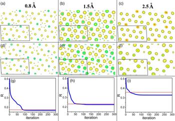
obs,h| even if the model is correct. When the high-resolution diffraction data are available and the trial phase set ϕ is correct (within certain accuracy), an EDM implemented in a particular way (e.g. electron density flipping in low-density regions as implemented in the charge flipping algorithm) results in very little difference between ρ and ρ*, therefore a small R factor is an indicator of the correctness of the electron density model. Nevertheless, when the resolution of the diffraction data is poor, electron density ripples because the truncation effect of Fourier synthesis will lead to considerable electron density out of the nuclear sites even the electron density model is correctly constructed using the correct phase set. Then an EDM, which usually take effect in low-density regions, will lead to significant difference between ρ and ρ*. We expect that the R factor will no longer be capable of indicating the correct model in such cases. This conjecture was confirmed by examining the evolution of R factor in successive EDM iterative cycles using simulated diffraction data at various resolutions. As shown in Figure 1, with the deterioration of the data resolution, R values for the correct electron density models increase, and so do the finally resultant R factors of iterative EDM cycles. In the case where the data resolution is 2.5 Å, the R value for the correct electron density model is significantly higher than the finally resultant one obtained from the iterative cycles. Clearly, in such a case, R factor defined in Eq. (2) is no longer capable of indicating the correct electron density model. We also note that R factor works well when the data of high resolution are available, and the correct model can be retrieved from the diffraction data by using the iterative EDM method. This implies that it might be unnecessary to find a better figure of merit for iterative EDM algorithms to monitor the evolution of electron density model in the successive iterative cycles, but we do need a new figure of merit different from R factor for identifying the correct electron density model when the data resolution is poor.
(color online) Electron density maps of C6Br6 at the resolutions of 0.8 (a), 1.5 (b), and 2.5 Å (c) constructed by Fourier synthesis using the structure amplitudes and correct phases. Shown in (d–f) are the resultant electron density models at the resolutions of 0.8, 1.5, and 2.5 Å, respectively, which are obtained from successive iterative EDM cycles. The structure amplitudes and correct phases are calculated from the structure data of C6Br6 reported by Wu et al. (Reference Wu, Spence, O'Keeffe and Groy2004). All electron density maps in (a–f) are projections of C6Br6 along [010] direction. The unit cell is represented by a parallelogram in each panel. Note that electron density models shown in (d–f) have origins different from that of the original structural model. Only electron density above a certain positive threshold is illustrated for clarity. (g–i) The evolution of R factor with the iterative EDM cycles. In each iterative cycle, non-negative electron densities are retained and the negative ones are reset to zero. The red horizontal line indicates the R value corresponding to the correct structure model. Panels (g–i) correspond to the iterative cycles using the simulated diffraction data of 0.8, 1.5, and 2.5 Å, respectively. Crystal data of C6Br6: P21/n, a = 8.381, b = 4.0192, c = 15.3939 Å, β = 92.674°, Z = 2.

We propose R Tian factor which is defined as
 $$R_{{\rm Tian}} = \displaystyle{{\mathop \sum \nolimits_{\rm h} \vert \vert F_{{\rm o,cal,h}}^* \vert - \vert F_{{\rm cal,h}}^* \vert \vert} \over {\mathop \sum \nolimits_{\rm h} \vert F_{{\rm o,cal,h}}^* \vert}} $$
where
 $F_{{\rm cal,}h}^* $
and
 $F_{{\rm o,cal,h}}^* $
represent the calculated structure factors obtained from the modified current and correct electron density models, respectively, to which the same EDM has been applied. When the trial phase set is correct within a certain accuracy, R
Tian will approach to zero. This holds true even for low-resolution data. The difficulty lies in that
 $\vert F_{{\rm o,cal,h}}^* \vert$
cannot be obtained before the correct electron density model is available. If a reasonable approximation of
 $\vert F_{{\rm o,cal,h}}^* \vert$
can be established using the available data, then R
Tian can be used as a figure of merit to identify the correct electron density model.
C. The estimation of R Tian factor
We suppose that the lattice parameters, the constituent atoms and their numbers in the unit cell are known together with the observed structure amplitudes before the structure determination. The number of atoms in the unit cell of the investigated crystal is assumed to be N, and the atomic scattering factor of the ith atom is supposed to be f i.
For a hypothetical structure which has the same unit cell as that of the investigated crystal and only one atom with an atomic scattering factor of f i at the origin, its structure factor can be readily calculated using the following equation
 $$F_{{\rm i,h}} = \mathop \sum \nolimits {f_{\rm i}} \times {\rm exp}( - 2\pi i\vec h \cdot \vec r) = f_{\rm i}. $$
The electron density map of the hypothetical structure ρ i can be calculated by a straightforward IFT, namely,
 $$\rho _{\rm i} = {\rm IFT(}F_{{\rm i},{\rm h}} {\rm )} = {\rm IFT}\; (\,f_{\rm i} ).$$
The Fourier synthesis in Eq. (5) is terminated at a resolution identical to that of the observed data of the investigated crystal. We suppose ρ
i changes into
 $\rho _{\rm i}^* $
after applying an imaginary EDM, then the structure factor of
 $\rho _{\rm i}^*, $
which is denoted as
 $F_{{\rm i},{\rm h}}^* $
, can be obtained by Fourier transform. We suppose the modification applied to ρ
i is V
i, then we have
 $$\rho _{\rm i}^* = \rho _{\rm i} \times V_{\rm i} $$
and
 $$F_{{\rm i},{\rm h}}^{\ast} = {\rm FT}(\rho _{\rm i}^{\ast}) = {\rm FT\;} \left(\rho _{\rm i} \times V_{\rm i} \right) = {\rm FT} (\rho _{\rm i}) \otimes {\rm FT} \left(V_{\rm i} \right) = f_{\rm i} \otimes v_{\rm i} $$
where ⊗ represents convolution, and v
i represents FT(V
i). In analogy to ρ
i, ρ
i
*
may be considered as the electron density map built up using a pseudo-atom at the origin with an atomic scattering factor
 $f_{\rm i}^* = f_{\rm i} \otimes v_{\rm i} $
, which is hereinafter referred to as pseudo-atomic scattering factor.
The imaginary EDM applied to ρ i is assumed to be
 $$V_{\rm i} = \left\{ {\matrix{ {1,\; \; \rho _{\rm i} \ge \delta _{\rm i}} \cr {0,\; \; \rho _{\rm i} \lt \delta _{\rm i}} \cr}} \right.$$
where δ
i is a real number close to 0. When δ
i is appropriately selected,
 $\rho _{\rm i}^* $
remains the same as ρ
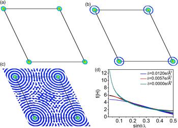
i only in a small region around the center of the atom and is set to zero in the rest regions. An example is given in Figure 2 to illustrate how
 $\rho _{\rm i}^* $
and
 $f_{\rm i}^* $
vary with δ
i. It can be clearly seen from Figure 2 that positive
 $\rho _{\rm i}^* $
is limited to the region very proximate to the atomic position even when δ
i is quite a small positive value. In addition, it is found that
 $f_{\rm i}^* $
varies significantly with δ
i, especially in the low sinθ/λ range. When δ
i is set to an appropriate value,
 $f_{\rm i}^* $
coincides with the original atomic scattering factor very well in the low sinθ/λ range, and only in the high sinθ/λ range significant difference between
 $f_{\rm i}^* $
and f
i can be observed. Since f
i value at θ = 0 represents the number of electrons of the ith atom,
 $f_{\rm i}^* $
coinciding with f
i in the low sinθ/λ range implies that the pseudo-atom has the same number of electrons as that of the ith atom at this δ
i value.
(color online) The dependence of
 ${\rm \;} \rho _{\rm i}^* $
and
 $f_{\rm i}^* $
on δ
i. (a–c) The modified electron density distributions on the (001) plane (at z = 0) of a hypothetical structure with only one carbon atom at origin. The colored regions have electron densities greater than δ
i. The original electron density map of the hypothetical structure is constructed at the resolution of 1 Å by using Eq. (5), and then modified according to Eqs (6) and (8). Maps shown in (a–c) correspond to the resultant electron density distributions modified with δ = 0.012, 0.0057, and 0.0 e/Å3, respectively. The hypothetical structure is derived from a known organic compound C252H326O19 reported by Czugler et al. (Reference Czugler, Weber, Parkanyi, Korkas and Bombicz2003). (d)
 $f_{\rm i}^* $
corresponding to δ = 0.0, 0.0057, and 0.012 e/Å3 and the atomic scattering factor of carbon (shown in black).

The “observed” electron density distribution of a crystal, ρ o, may be considered as the superposition of electron density of each constituent atom in the unit cell, which can be represented by
 $$\rho _{\rm o} = \mathop \sum \limits_{\rm i}^N \rho _{\rm i} (r_{\rm i} )$$
where ρ i(r i) is ρ i translated from the origin to the atomic position r i.
We assume
 $$\rho _{\rm o}^* = \rho _{\rm o} \times \mathop \sum \limits_{\rm i}^N V_{\rm i} (r_{\rm i} ) = \mathop \sum \limits_{\rm i}^N \rho _{\rm i} (r_{\rm i} ) \times \mathop \sum \limits_{\rm j}^N V_{\rm j} (r_{\rm j} )$$
where V i(r i) is V i translated from the origin to the atomic position r i.
It is achievable that the region with V j (r j) = 1 of each atom does not overlap with that of adjacent atoms by selecting appropriate δ i. In such cases,
 $$\rho _{\rm i} (r_{\rm i} ) \times V_{\rm j} (r_{\rm j} ) = 0$$
for i ≠ j
Then we obtain
 $$\rho _{\rm o}^* = \mathop \sum \limits_{\rm i}^N \rho _{\rm i} (r_{\rm i} ) \times V_{{\rm i}\;} \left( {r_{\rm i}} \right) = \mathop \sum \limits_{\rm i}^N \rho _{\rm i}^* (r_{\rm i} )$$
and
 $$F_{{\rm o},{\rm cal},{\rm h}}^* = {\rm FT(}\rho _{\rm o}^* {\rm )} = \mathop \sum \limits_{\rm i}^N f_{\rm i}^* {\rm exp}( - 2\pi i\vec h \cdot \overrightarrow {r_{\rm i}} )$$
The experimental observed diffraction intensity of a crystal is given by
 $$\eqalign{\left \vert {F_{{\rm obs},{\rm h}}} \right \vert ^2 & = K\mathop \sum \limits_{\rm i}^N \mathop \sum \limits_{\rm j}^N f_{\rm i} f_{\rm j} \exp \left[ {2\pi i\vec h \cdot \left( {\overrightarrow {r_{\rm i}} - \overrightarrow {r_{\rm j}}} \right)} \right] \cr & = K\{ \mathop \sum \limits_{\rm i}^N f_{\rm i}^2 + \mathop \sum \limits_{\rm i}^N \mathop \sum \limits_{{\rm j}\left( {{\rm i} \ne {\rm j}} \right)}^N f_{\rm i} f_{\rm j} \exp \left[ {2\pi i\vec h \cdot \left( {\overrightarrow {r_{\rm i}} - \overrightarrow {r_{\rm j}}} \right)} \right]\} \cr & = K\mathop \sum \limits_{\rm i}^N f_{\rm i}^2 \left\{ {1 + \displaystyle{{\mathop \sum \nolimits_{\rm i}^N \mathop \sum \nolimits_{{\rm j}({\rm i} \ne {\rm j})}^N f_{\rm i} f_{\rm j} {\rm exp}\left[ {2\pi i\vec h \cdot \left( {\overrightarrow {r_{\rm i}} - \overrightarrow {r_{\rm j}}} \right)} \right]} \over {\mathop \sum \nolimits_{\rm i}^N f_{\rm i}^2}}} \right\}} $$
where K is a scale factor independent of θ. According to Eq. (13), the intensity of the imaginary crystal with the electron density distribution
 $\rho _{\rm o}^* $
should be
 $$\eqalign{&\left \vert {F_{{\rm o},{\rm cal},{\rm h}}^*} \right \vert ^2 \cr &\quad = K\mathop \sum \limits_{\rm i}^N f_{\rm i}^{*2} \left\{ {1 + \displaystyle{{\mathop \sum \nolimits_{\rm i}^N \mathop \sum \nolimits_{{\rm j}\left( {{\rm i} \ne {\rm j}} \right)}^N f_{\rm i}^* f_{\rm j}^* \exp \left[ {2\pi i\vec h \cdot \left( {\overrightarrow {r_{\rm i}} - \overrightarrow {r_{\rm j}}} \right)} \right]} \over {\mathop \sum \nolimits_{\rm i}^N f_{\rm i}^{*2}}}} \right\} \cr & \quad = K\mathop \sum \limits_{\rm i}^N f_{\rm i}^{*2} \left\{ {1 + \displaystyle{{\mathop \sum \nolimits_{\rm i}^N \mathop \sum \nolimits_{{\rm j}({\rm i} \ne {\rm j})}^N k_{\rm i} k_{\rm j} f_{\rm i} f_{\rm j} {\rm exp}\left[ {2\pi i\vec h \cdot \left( {\overrightarrow {r_{\rm i}} - \overrightarrow {r_{\rm j}}} \right)} \right]} \over {\mathop \sum \nolimits_{\rm i}^N k_{\rm i}^2 f_{\rm i}^2}}} \right\}} $$
where k
i =
 $f_{\rm i}^* /f_{\rm i} $
and k
j =
 $f_{\rm j}^* /f_{\rm j} $
. If k
i = k
j, then we obtain
 $$\left \vert {F_{{\rm o},{\rm cal},{\rm h}}^*} \right \vert ^2 = \displaystyle{{\mathop \sum \nolimits_{\rm i}^N f_{\rm i}^*2} \over {\mathop \sum \nolimits_{\rm i}^N f_{\rm i}^2}} \left \vert {F_{{\rm obs},{\rm h}}} \right \vert ^2 $$
As discussed above,
 $f_{\rm i}^* $
can coincide with f
i in the low θ range when δ
i is appropriately set. This implies that in such cases k
i = k
j = 1 and Eq. (15) is valid. At high θ angle, k
i = k
j seems to be a prerequisite hard to meet. Nevertheless, we note that Eq. (15) agrees well with results derived from Wilson distribution (Wilson, Reference Wilson1942), which is described by
 $${\lt}\left \vert {F_{{\rm obs},{\rm h}}} \right \vert ^2{\gt} = K^{\prime} \mathop \sum \limits_{\rm i}^N f_{\rm i}^2 $$
where <|F obs,h|2> is the averaged |F obs,h|2 over a given range of sin2 θ, and K ′ is a scale factor independent of θ. Eq. (16) is valid when λ/sinθ is small compared with the inter-atomic distances. Similarly, the following equation
 $${\lt}\left \vert {F_{{\rm o},{\rm cal},{\rm h}}^*} \right \vert ^2{\gt} = K^{\prime} \mathop \sum \limits_{\rm i}^N f_{\rm i}^{*2} $$
is valid when λ/sinθ is small. Combining Eqs (16) and (17), we obtain
 $${\lt}\left \vert {F_{{\rm o},{\rm cal},{\rm h}}^*} \right \vert ^2{\gt} = \displaystyle{{\mathop \sum \nolimits_{\rm i}^N f_{\rm i}^{*2}} \over {\mathop \sum \nolimits_{\rm i}^N f_{\rm i}^2}} {\lt}\left \vert {F_{{\rm obs},{\rm h}}} \right \vert ^2{\gt} $$
Although the validity of Eq. (18) does not mean that Eq. (15) is valid, it implies that estimating
 $\left\vert {F_{{\rm o},{\rm cal},{\rm h}}^*} \right\vert^2 $
using Eq. (15) is statistically reasonable.
Combining Eqs (3) and (15), we obtain
 $$\eqalign{ R_{{\rm Tian}} &= \displaystyle{{\mathop \sum \nolimits_{\rm h} \vert \vert F_{{\rm o},{\rm cal},{\rm h}}^* \vert - \vert F_{{\rm cal},{\rm h}}^* \vert \vert} \over {\mathop \sum \nolimits_{\rm h} \vert F_{{\rm o},{\rm cal},{\rm h}}^* \vert}} \cr & = \displaystyle{{\mathop \sum \nolimits_{\rm h} \vert \sqrt {\displaystyle{{\mathop \sum \nolimits_{\rm i}^N f_{\rm i}^{*2}} \over {\mathop \sum \nolimits_i^N f_i^2}} \left \vert {F_{{\rm obs},{\rm h}}} \right \vert ^2} - \vert F_{{\rm cal},{\rm h}}^* \vert \vert} \over {\mathop \sum \nolimits_{\rm h} \sqrt {\displaystyle{{\mathop \sum \nolimits_{\rm i}^N f_{\rm i}^{*2}} \over {\mathop \sum \nolimits_{\rm i}^N f_{\rm i}^2}} \left \vert {F_{{\rm obs},{\rm h}}} \right \vert ^2}}}} $$
Note that EDM applied to both the correct and the current electron density models should be the same in Eq. (3). In Eq. (19), we actually have assumed that the multiplier applied to modify the correct electron density model is
 $\sum\nolimits_{\rm i}^N {V_{\rm i} (r_{\rm i} )} $
by taking
 $\sqrt {\left( {\mathop \sum \nolimits_{\rm i}^N f_{\rm i}^{*2} /\mathop \sum \nolimits_{\rm i}^N f_{\rm i}^2} \right)\left\vert {F_{{\rm obs},{\rm h}}} \right\vert^2} $
as the approximation of
 $\vert F_{{\rm o},{\rm cal},{\rm h}}^* \vert$
. Therefore, the current electron density model should be modified by multiplying it with
 $\sum\nolimits_{\rm i}^N {V_{\rm i} (r_{\rm i} )} $
. Unfortunately,
 $\sum\nolimits_{\rm i}^N {V_{\rm i} (r_{\rm i} )} $
contains the atomic position r
i and cannot be determined prior to the structure determination. An alternative way to modify the current electron density model is multiplying it with
 $$W = \left\{ {\matrix{ {1,\; \; \rho \ge \delta _{{\rm cryst}}} \cr {0,\; \; \rho \lt \delta _{{\rm cryst}}} \cr}} \right.$$
where δ
cryst is a real number. Clearly,
 $\vert F_{{\rm cal},{\rm h}}^* \vert$
varies with both the trial phase set and δ
cryst. When the modified current electron density map ρ* = ρW is close to the modified correct electron density map
 $\rho _{\rm o}^* = \sum\nolimits_{\rm i}^N {\rho _{\rm i} (r_{\rm i} ) \times V_{{\rm i}\;} (r_{\rm i} )} $
, R
Tian calculated with Eq. (19) reaches the minimum, ideally, zero.
III. DISCUSSION
A. The validity of the method to estimate
$\left\vert {F_{{\rm o},{\rm cal},{\rm h}}^*} \right\vert$

The validity of the method to estimate
 $\left\vert {F_{{\rm o},{\rm cal},{\rm h}}^{\rm *}} \right\vert$
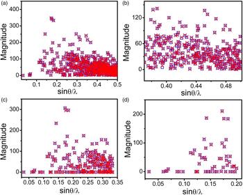
using Eq. (15) is tested on simulated diffraction data, which are obtained from the known structure of C6Br6 (Wu et al., Reference Wu, Spence, O'Keeffe and Groy2004). Electron density maps with the resolution of 1.0, 1.5, and 2.5 Å are calculated by IFT. At each data resolution, δ
C and δ
Br are appropriately set to satisfy the condition that
 $f_{\rm i}^* $
coincides with f
i approximately in the low sinθ/λ region. Then the theoretical values of
 $\left\vert {F_{{\rm o},{\rm cal},{\rm h}}^{\rm *}} \right\vert$
are calculated using Eq. (14) and shown in Figure 3 as red crosses. The estimated values of
 $\left\vert {F_{{\rm o},{\rm cal},{\rm h}}^{\rm *}} \right\vert$
are calculated using Eq. (15) and presented in Figure 3 as blue squares. As shown in Figure 3, at each data resolution, the estimated
 $\left\vert {F_{{\rm o},{\rm cal},{\rm h}}^*} \right\vert$
values agree well with the theoretical ones. To derive Eq. (15) from Eq. (14), we have assumed that atomic scattering factors of different atoms vary by the same proportion as a result of EDM. It seems to be a condition hard to be satisfied. Nevertheless, tests on simulated diffraction data of C6Br6 indicated that Eq. (15) is valid in estimating
 $\left\vert {F_{{\rm o},{\rm cal},{\rm h}}^*} \right\vert$
even there are atoms with significantly different scattering power, such as C and Br, in the unit cell. On the other hand, we also would like to explicitly state that Eq. (15) can only be applied to estimate the structure amplitudes of an electron density map modified in a specific way, which has been described in details in Section II C.
(color online)
 $\left\vert {F_{{\rm o},{\rm cal},{\rm h}}^*} \right\vert$
calculated using Eq. (14) (red cross) and (15) (blue square) of C6Br6. (a) Data resolution: 1.0 Å, δ
C = 0.0018 e/Å3, δ
Br = 0.125 e/Å3; (b) is an enlarged view of the bottom-right region of (a). (c) Data resolution: 1.5 Å, δ
C = 0.003 e/Å3, δ
Br = 0.07 e/Å3; (d) Data resolution: 2.5 Å, δ
C = 0.0024 e/Å3, δ
Br = 0.021 e/Å3.

B. The validity of R Tian in identifying the correct phase set
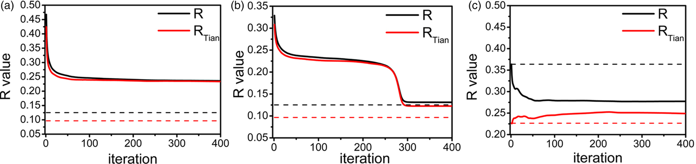
The factor R Tian is aimed to identifying the correct phase set from a great number of possible phase sets assigned to the observed structure amplitudes. The capability of R Tian in evaluating the trial phase sets is tested on simulated diffraction data of known structure C252H326O19 (Czugler et al., Reference Czugler, Weber, Parkanyi, Korkas and Bombicz2003). Two data sets at the resolution of 1.0 and 2.5 Å, respectively, are generated. Four hundred iterative EDM cycles are performed to retrieve the correct electron density model from the simulated data set at the resolution of 1.0 Å. The initial electron density models are constructed by FT using the “observed” structure amplitudes and random phases. In each following iterative cycle, electron densities greater than δ cryst are retained, and the others are set to zero. The variation of R and R Tian factors with the iterative EDM cycles is shown in Figure 4(a). Both R and R Tian drop drastically at the early stage and then keep stable in the following iterative cycles. The convergent R and R Tian values coincide with each other, and both are much higher than the expected values for the correct model. It is noteworthy that the expected value of R Tian is lower than that of R factor. In this case, the correct model cannot be retrieved by iterative EDM cycles, as indicated by the high convergent R and R Tian values. Then a partial structure including 10 correctly located carbon atoms is build up, and a phase set is derived from this partial structure. This phase set is combined with the “observed” structure amplitudes to generate the initial electron density model. Starting with this initial electron density model, iterative EDM cycles converge to the correct electron density map. The evolution of R and R Tian factors in this attempt is shown in Figure 4(b). In this case, the convergent R value approaches to the expected value for the correct model, while the convergent R Tian value is still significantly higher than the expected value for the correct model. The discrepancy between the convergent and the expected value of R Tian is because of the difference between the convergent and the correct electron density models. This indicates that R Tian is more sensitive than R to the variation of electron density models. At the resolution of 2.5 Å, we use the correct phase set to establish the initial electron density model for the iterative EDM cycles. The evolution of R and R Tian in this case is shown in Figure 4(c). The R factor decreases considerably with the iterative cycles, while R Tian increases significantly in the same process. This indicates clearly that R factor is no longer valid at this resolution, but R Tian is still valid for identifying the correct phase set. In addition, we note that R Tian is lower than R for the correct model at both data resolution, and the latter increases faster than the former when the data resolution deteriorates.
(color online) The variation of R and R Tian factors with the iterative EDM cycles at the resolution of 1.0 (a, b) and 2.5 Å (c). The initial electron density model in (a) is generated using random phases while in (b) it is generated using phase set derived from the partial structure. In (c) the correct electron density map of C252H326O19 is used as the initial model. In each panel, the target values of R and R Tian corresponding to the correct electron density maps are shown as black and red horizontal dotted lines, respectively. δ cryst is set to zero in all iterative EDM cycles.

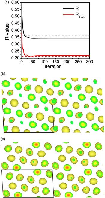
Tests are also performed on the simulated data of C6Br6 at the resolution of 2.5 Å. The variation of R Tian and R with the iterative EDM cycles is shown in Figure 5(a). The initial electron density model was generated by IFT using the “observed” structure amplitudes and the random phases. As discussed in Section II B, the R factor is no longer valid in identifying the correct electron density model in this case. It is interesting to note that R Tian reaches a minimum during the iterative process, which is close to the expected value for the correct electron density model. The electron density model corresponding to the minimum value of R Tian is presented in Figure 5(b). Comparison between this model and the correct electron density map [shown in Figure 5(c)] reveals that it is a close resemblance to the correct map. This example further confirms that R Tian is still valid in identifying the correct electron density model at a resolution of 2.5 Å. Moreover, R Tian seems to be more sensitive than R factor because it varies more significantly than R, especially when an approximately correct model has been obtained.
(color online) (a) The variation of R and R Tian factor with the iterative EDM cycles at the resolution of 2.5 Å. δ cryst is set to zero in the iterative EDM cycles. Black and red dotted lines indicate the R and R Tian values for the correct electron density map, respectively. (b) The electron density model corresponding to the minimum value of R Tian. (c) The correct electron density map of C6Br6 at the resolution of 2.5 Å. Both (b) and (c) are projections along [010] direction. Only electron densities above 2.5 e/Å3 are illustrated for clarity.

C. Application of R Tian in structure determination
In Section III B, we have checked the capability of R Tian in identifying correct phase set by investigating its variation with the iterative EDM cycles. This does not mean that the R Tian factor is designed for iterative EDM algorithms. Usually, iterative EDM algorithms work only in cases where the high-resolution diffraction data are available. In such cases, R Tian is only slightly different from R factor numerically, and R factor can be more readily calculated than R Tian. R Tian factor is independent of iterative EDM algorithms. For an arbitrary trial phase set assigned to the observed structure amplitudes, R Tian can be estimated approximately. The correct phase set is supposed to have the lowest R Tian value. Tests on simulated diffraction data indicate that R Tian is valid even at the resolution of 2.5 Å. Clearly, since the number of all possible phase sets is tremendous, it is not realistic to estimate R Tian values for all possible phase sets and then pick out the phase set with the lowest R Tian value. Potentially, R Tian may be applied as a goal function of global optimization algorithms for retrieving the electron density map from data set of poor resolution.
Acknowledgements
This work was financially supported by the National Natural Science Foundation of China (Grant Nos. 11574060 and 11474281). HL and MH are very grateful to Guang-Lian Tian for her consistent support and encouragement.