

Introduction
The global population is projected to reach 9.8 billion by 2050, with food demand expected to increase by 50% relative to 2019 (FAO 2023; WRI 2019). This challenge is compounded by various uncertainties, including climate change, resource depletion, and potential disruptions to supply chains, as evidenced by the COVID-19 pandemic. Previous studies demonstrate that official forecasts of production released by government agencies have a significant impact on markets and decisions within supply chains (Adjemian Reference Adjemian2012; Irwin et al. Reference Irwin, Gerlow and Liu1994; Isengildina et al. Reference Isengildina, Irwin and Good2006; Isengildina-Massa et al. Reference Isengildina-Massa, Cao, Karali, Irwin, Adjemian and Johansson2021).
The Global Food Assessment (GFA) report, published annually by the USDA’s Economic Research Service, provides one-year and ten-year projections for low- and middle-income countries, focusing on grain demand, production, and the Implied Additional Supply Required (IASR), which measures the gap between demand and domestic production (Zereyesus et al. Reference Zereyesus, Cardell, Valdes, Ajewole, Zeng, Beckman, Ivanic, Hashad, Jelliffe and Kee2022b). Our study aims to explore and evaluate alternative methods for improved long-term grain forecasting, specifically for the GFA utilized in the USDA’s GFA grain supply model.
The USDA’s long-term agricultural projections represent a departmental consensus on a long-term representative scenario for the agricultural sector over the next decade. Both the USDA Long-term Agricultural Projections (U.S. Department of Agriculture 2025) and the USDA GFA (Zereyesus et al. Reference Zereyesus, Cardell, Farris, Ajewole, Johnson, Lin, Valdes and Zeng2025) reports utilize a 10-year projection period to offer a comprehensive outlook that assists producers, policymakers, and market participants in making informed decisions. Our paper also adopts a 10-year forecast horizon, consistent with these reports (U.S. Department of Agriculture 2025; Zereyesus et al. 2025). While the model developed in this work is relevant to wide applications and other countries, we restrict our analyses to the low- and middle-income countries covered by the GFA assessment.
Previous work by Zereyesus et al. (Reference Zereyesus, Baquedano and Morgan2022a) evaluates the GFA supply forecasting model using a cross-validation approach to select the best model specification for forecasting yield, showing that models at the subregional level improved yield prediction. This disaggregation allows for more granular analysis, capturing regional variations in yield that affect overall grain supply. The projections of grain supply are then combined with projections of demand for grains (both food and non-food) to calculate the gap between demand and supply, crucial for assessing food security and identifying areas needing food aid or trade opportunities.
Despite its recent advancements, the existing model used by USDA GFA can be extended to improve its effectiveness for long-term forecasting. First, from a modeling perspective, both the long-term grain yield and area projections use pooled panel data models across countries to estimate the relationship between yield and area and their long-term influencing factors. Yield is modeled as a function of return to inputs, technological improvement, and country-specific factors. Area is modeled as a function of lagged area, expected crop and fertilizer prices, and a time trend (Zereyesus et al. Reference Zereyesus, Cardell, Valdes, Ajewole, Zeng, Beckman, Ivanic, Hashad, Jelliffe and Kee2022b). For both yield and area projections, we explore a wide range of regression model specifications varying in predictor variables (e.g., prices, temperature, precipitation), coefficient pooling (pooled vs. country-specific), fixed effects, functional forms (linear vs. Poisson), and trend structures (linear vs. non-linear using natural cubic splines) as well as country-specific Autoregressive Integrated Moving Average with exogenous variables (ARIMAX) models. This exhaustive modeling framework ensures that we consider a broad set of specifications that can improve forecast accuracy. The model’s suitability for long-term forecasting, particularly for 10 years into the future, has not been rigorously validated against alternative models. This lack of comparative analysis is particularly important given the nature of the projection and the need for rigorous cross-validation approaches that account for the time series nature of the forecasting exercise. We develop a time-series out-of-sample validation approach specifically for long-term forecasting, considering the current model’s potential inadequacy for extended horizons.
We utilize a data-driven time-series out-of-sample validation to select the model specification that provides the best 10-year forecast. By using out-of-sample validation, we avoid overfitting that can occur using in-sample metrics like the in-sample R 2. Our methodology also explicitly accounts for the time-series nature of the data to avoid overstating forecast performance. Our methodology is generalizable and it can be implemented with different data to provide reliable forecasts of supply.
We evaluate alternative statistical methods for forecasting international grain supply over a 10-year horizon. We first estimate the models for area and yield separately and assess the model accuracy. The model specifications that perform best for area do not necessarily correspond with the model specifications that perform best for yield. More specifically, we focus on regression models with varying specifications (pooled vs. country-specific coefficients, linear vs. non-linear trends, and alternative predictors) and country-specific ARIMAX models with different ARIMA orders (p, d, q) and predictor variables. This ARIMAX approach is motivated by several key factors influencing grain supply. First, temperature and precipitation patterns can significantly affect grain supply and agricultural productivity. Second, understanding heterogeneous and potentially non-linear yield trends across countries is crucial for accurate long-term forecasting. Third, grain supply responds to prices.
Our work modeling international grain supply draws on several areas of prior research. First, the established literature highlights the significant impact of weather change on global agricultural production. Studies consistently demonstrate that changes in temperature and precipitation can negatively affect grain production, yield, and overall agricultural Total Factor Productivity (TFP) (Ceglar et al. Reference Ceglar, Toreti, Prodhomme, Zampieri, Turco and Doblas-Reyes2018; Lobell et al. Reference Lobell, Schlenker and Costa-Roberts2011; Ortiz-Bobea et al. Reference Ortiz-Bobea, Ault, Carrillo, Chambers and Lobell2021). For instance, concurrent heat stress and droughts have been shown to account for inter-annual maize yield variability (Ceglar et al. Reference Ceglar, Toreti, Prodhomme, Zampieri, Turco and Doblas-Reyes2018), and climate change has reduced the growth rate of global agricultural TFP by approximately 21 percent since 1961 (Ortiz-Bobea et al. Reference Ortiz-Bobea, Ault, Carrillo, Chambers and Lobell2021). The literature also suggests that improved forecasting systems for seasonal climatic conditions can mitigate these adverse effects (Hansen Reference Hansen2012; Jones et al. Reference Jones, Hansen, Royce and Messina2000; Mase and Prokopy Reference Mase and Prokopy2014).
Second, prior studies examine heterogeneous and potentially non-linear yield trends across countries to forecast future global food supply (Grassini et al. Reference Grassini, Eskridge and Cassman2013; Ray et al. Reference Ray, Ramankutty, Mueller, West and Foley2012). Understanding these trends is crucial for assessing potential future grain supply and growth rates, which are essential for policy and food security considerations. Hafner’s (Reference Hafner2003) analysis, for example, demonstrates that yield growth across numerous nations is not constrained by fundamental physiological limitations.
Third, research explores the responsiveness of global supply to price fluctuations (Haile et al. Reference Haile, Kalkuhl and von Braun2014; Haile et al. Reference Haile, Brockhaus and Kalkuhl2016; Hendricks et al. Reference Hendricks, Janzen and Smith2015; Roberts and Schlenker Reference Roberts and Schlenker2013). Studies indicate that higher futures prices can stimulate an expansion in global crop supply, although grain price volatility can act as a deterrent (Haile et al. Reference Haile, Kalkuhl and von Braun2015). Additionally, global acreage adjustments in response to international crop prices, price risks, input costs, and temporal trends have been documented (Haile et al. Reference Haile, Kalkuhl and von Braun2014). However, it is important to note that these studies primarily aim to estimate supply elasticities for policy analysis rather than focusing on direct supply forecasting.
While the machine learning literature offers valuable insights into crop yield prediction, particularly with the integration of high-resolution climate and satellite data, our study primarily focuses on traditional time-series non-machine learning methodologies. Studies (e.g., Cai et al. Reference Cai, Guan, Lobell, Potgieter, Wang, Peng, Xu, Asseng, Zhang, You and Peng2019; Feng et al. Reference Feng, Wang, Liu, Waters, Xiao, Shi and Yu2020; Fillipi et al. Reference Filippi, Jones, Wimalathunge, Somarathna, Pozza, Ugbaje, Jephcott, Paterson, Whelan and Bishop2019; Johnson et al. Reference Johnson, Hsieh, Cannon, Davidson and Bédard2016; Li et al. Reference Li, Zhang, Wang, Feng, He, Shi, Liu, Harrison, Liu, Yao, Li, He, Feng, Siddique and Yu2023; and Roznik et al. Reference Roznik, Mishra and Boyd2023) demonstrate the potential of machine learning models like Random Forest, Support Vector Machines, Artificial Neural Networks, and XGBoost to achieve high accuracy in yield forecasting. These models often outperform traditional regression-based approaches. On the other hand, Roznik et al. (Reference Roznik, Mishra and Boyd2023) estimate corn yield forecasts using satellite and weather data employing XGBoost, and their results indicate that XGBoost models have a similar accuracy forecast to the current World Agricultural Supply and Demand Estimates corn yield forecasts, which are based on survey methodology. In our specific context, initial analyses indicate relatively better performance from traditional time-series models given the aggregate, annual nature of our data. Therefore, given the performance of traditional time series models in this specific use case, our research prioritizes these methodologies. Nevertheless, we acknowledge the importance and relevance of machine learning in the broader field of agricultural forecasting and recognize its potential for future applications.
Data
We collect production, area, prices, and weather data across 78 countries from 1980 to 2021 for six major crops: corn, sorghum, millet, barley, wheat, and rice. The most recent GFA report that USDA assembles each year includes 83 countries; however, we use 78 countries in our analysis due to data limitations of some countries that are discussed in more detail in the Supplementary Appendix.
Production, Area, and Yield: We obtain production and harvested area from the USDA Foreign Agricultural Service Production, Supply and Distribution (PSD) database. The unit for production is millions of kilocalories (kcal), area is in hectares, and yield is in millions of kilocalories per hectare. While PSD has production data in metric tons, we convert to calories using the caloric equivalents from FAOSTAT (2024), allowing us to aggregate production across crops. Aggregation by caloric content is primarily intended to enable comparison of the main grains across countries, based on the caloric content of grains in each country, regardless of the specific types of grain crops. Although crop-specific analysis has been utilized (e.g., Zereyesus et al. Reference Zereyesus, Baquedano and Morgan2022a), food security assessment involves analyzing large and complex data sets. Regarding the choice between aggregating by calorie content versus by volume of grain, although both are relevant and useful, we choose to aggregate by caloric content to account for the fact that some grains have a higher caloric density. This approach simplifies the findings for stakeholders interested in a food security assessment and is consistent with previous literature (e.g., Hendricks et al. Reference Hendricks, Janzen and Smith2015; Roberts and Schlenker Reference Roberts and Schlenker2013). Yield is calculated as total grain production (Millions of kcal) divided by total area (Hectares).
Prices: Our model specifications consider two different measures of crop prices as predictor variables in the model specifications: futures prices from the International Grains Council and spot prices from the World Bank commodity price database. We use futures and spot prices a month before planting for each crop since they are the most relevant prices, as farmers make most production decisions before planting a crop and it avoids endogeneity concerns (Haile et al. Reference Haile, Kalkuhl and von Braun2015; Hendricks et al. Reference Hendricks, Janzen and Smith2015). To construct crop prices relevant to the crop season of each country, we use the United Nations Food and Agriculture Organization Global Information and Early Warning System (GIEWS), which provides planting months for different countries and crops. However, some countries do not have specified planting months, so we spatially interpolate these missing planting months using nearest neighbor interpolation. Then, we aggregate prices across crops using a simple and weighted average to derive an average annual grain price for each country. For the weighted average, the weights represent a share of grain production for the specific crop between 1990 and 1999, so that the price of grains in a country reflects the price of crops with greater production. Futures and spot prices are in USD per million kilocalories.
Weather: Annual and monthly weather data at the country level are obtained from the Climatic Research Unit (CRU) at the University of East Anglia. CRU creates monthly country-level data by averaging monthly gridded weather data within each country. We use the cumulative precipitation (mm) and the average temperature (°C) for each month and year.
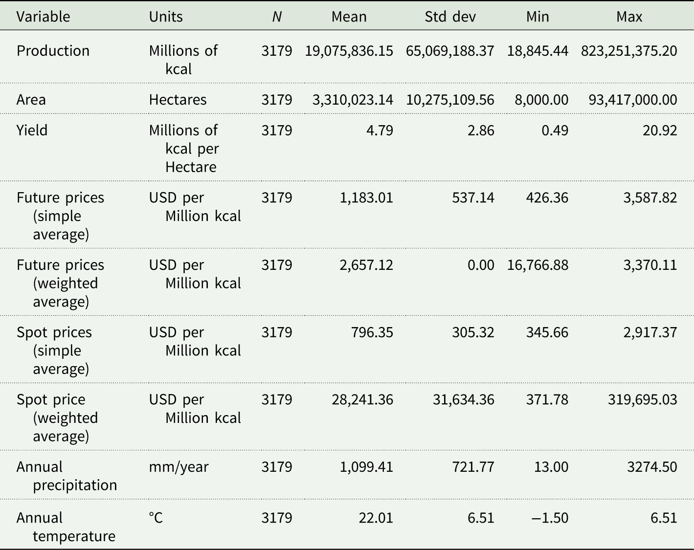
The summary statistics in Table 1 are from the final data set used to forecast production that spans from 1980 to 2021 for 78 countries. It is important to highlight that not all countries produce the same crops, so even if some crop price measures are global, they will differ across countries due to different crops being produced and different planting seasons. The average production in our data set is 19,075,836 million kilocalories, with an average harvested area of 3,310,023 hectares and an average yield of 4.8 million kcal per hectare.
Summary statistics of data (1980–2021)
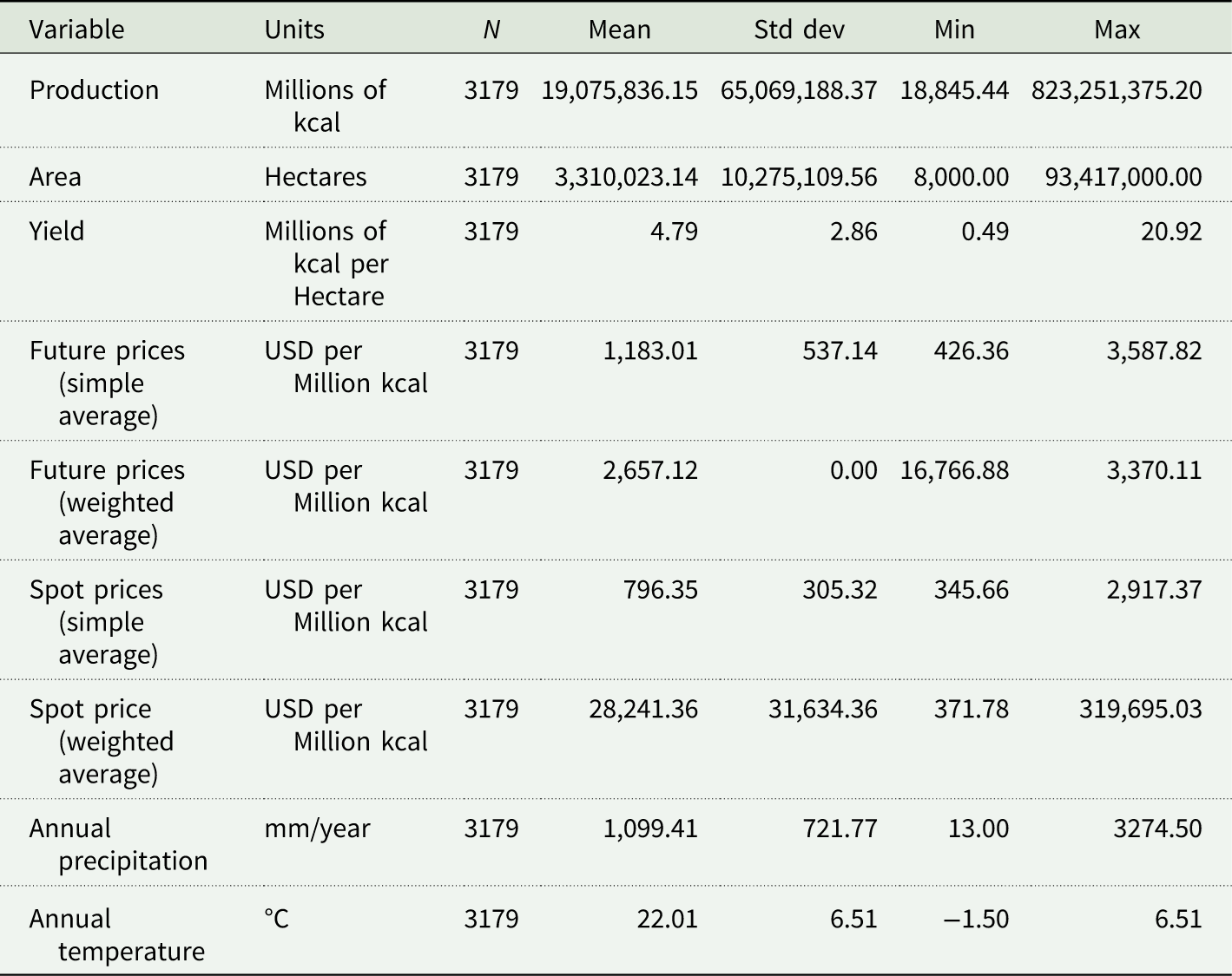
Table 1. Long description
The table has seven columns, Variable Name, Units, N, Mean, Standard Deviation, Minimin and Maximum. It show the values of nine variables.
Note: Summary statistics are across 78 countries over the period 1980–2021. Production and prices of grains are aggregated across corn, sorghum, millet, barley, wheat, and rice using the caloric content of each grain. Production data are from FAO, futures prices are from the Chicago Board of Trade, spot prices are from the World Bank, and weather data are from the Climatic Research Unit (CRU) at the University of East Anglia.
Methods
Our modeling methodology aims to find the best specification for out-of-sample forecasting of grain production. We estimate country-specific models but using the same model specification. We establish a general model specification and evaluate several variations to accomplish this objective. Note that for our analysis, we aggregate the production of six grains (barley, corn, rice, millet, sorghum, and wheat) using caloric equivalents, rather than modeling the production of individual crops. The following part of this section provides a general description of the models estimated in this study. Lastly, we describe our out-of-sample validation methodology to assess model performance.
Decomposition of production forecasts
Our approach to forecast grain production employs the decomposition of production into two components: harvested area and yield (i.e., production per unit of area). This is written as
 ${Prod_{i,t}}=Are{a_{i,t}}\;*\;Yiel{d_{i,t,}}$
where Prodit is the production in country i and year t, Areait is the harvested area, and Yieldit is the yield. We estimate separate models to forecast Areait and Yieldit . Then we generate a forecast of production by multiplying the forecast of Areait times the forecast of Yieldit .
Regression models
The general econometric specification to forecast production using regression models is written as:
 ${Y_{i,t}}=f\left( {t,{\theta _i}} \right)+{\beta _i}{X_{i,t}}+{\alpha _i}+{\varepsilon _{i,t,}}$
where Yit denotes the dependent variable: either Area (Millions of Hectares) or Yield (Millions of kcal per Hectare); f (t, θi ) denotes a trend that could either be linear or non-linear; βi are the coefficients for each predictor variable; Xit are the predictor variables (i.e., futures prices, spot prices, temperature, and precipitation.); αi are country-fixed effects; and ϵit are the residuals. In the most general specification, we allow country-specific trends and country-specific coefficients on predictors so that the coefficients have an i subscript, θi and βi .
Note that our objective is to forecast production into the future and not to provide causal estimates of how different factors affect production. Therefore, we do not impose economic theory on the specification. Instead, we keep the specification as flexible as possible and allow out-of-sample prediction errors to guide the model selection. Next, we summarize each of the variations on the general model specification in Equation (2) that we consider.
Linear versus Non-linear Trends: We include the possibility of a trend in our specifications to account for technological improvements over time in crop yields. Trends might also be present in crop area due to policies that affect land area and technological improvements that make crop area more or less profitable over time. The trend is either assumed to be linear or a flexible non-linear function. When a non-linear relationship is allowed, we use a natural cubic spline with three knots. Natural cubic splines have several advantages over polynomials in that they allow non-symmetric, non-linear trends with relatively few parameters estimated (James et al. Reference James, Witten, Hastie and Tibshirani2013).
Predictor Variables: We consider specifications with different predictors included in Xit . One option that we consider is to have no additional controls and model production simply according to trends. We also consider different combinations of prices, precipitation, and temperature as predictors. Prices could affect both area and yield due to the supply response of producers. We consider both futures and spot prices because it is not clear a priori which measure will best capture prices affecting producer decisions. Temperature and precipitation could obviously impact yields but can also impact growing area through crop failure (Cui Reference Cui2020; Obembe Reference Obembe, Hendricks and Tack2021). However, we do not impose a restriction that any of these variables must be included in the model because they could have low predictive power and worsen the out-of-sample prediction accuracy.
Pooled versus Country-Specific Coefficients: We estimate a single coefficient for each of the predictors (i.e., pooled) or we allow the coefficients to differ across countries. Pooled coefficients effectively reduce the number of predictors and can improve accuracy if coefficients are homogeneous. Country-specific coefficients allow more flexibility in the model.
Fixed Effects: The specifications also include some that have a common intercept across countries and others with country-specific intercepts (i.e., country fixed effects), sub-regional intercepts, or regional intercepts. Similar to country-specific coefficients, fixed effects allow more flexibility in the model but increase the number of parameters estimated.
All 928 combinations of predictors, pooled versus country-specific coefficients, and fixed effects that we consider in this study are illustrated in Tables A1 and A2 in the Supplementary Appendix.
Linear versus Poisson: We also estimate all 928 regressions using ordinary least squares (OLS) and a Poisson regression to allow different functional forms for how the predictors impact production. Poisson uses the functional form Yit = exp (·), which is similar to an OLS model where the dependent variable is a natural logarithm (i.e., ln(Yit )). While the linear specification assumes that a change in the predictor affects the dependent variable by a certain number of units, the Poisson specification assumes that a change in the predictor affects the dependent variable by a certain percentage.
To summarize, we fit all 928 model specifications with area as the dependent variable and again with yield as the dependent variable. We then fit each model using both OLS and Poisson models and with linear and nonlinear trends.
ARIMAX model
We also estimate country-specific Autoregressive Integrated Moving Average models with exogenous variables (ARIMAX). ARIMAX models account for the historical information of a series using autoregression, moving averages, and differencing (Box and Jenkins Reference Box and Jenkins1970). Also, we include the effect that one or more exogenous variables have on the stationary variable Yt . According to Hyndman and Athanasopoulos (Reference Hyndman and Athanasopoulos2018), the ARIMAX model is written as
 $Y_{i,t}={\sum }_{\tau =1}^{p} \varnothing _{i}Y_{i,t-\tau }+{\sum }_{\tau =1}^{q}{\varphi _{i}}\varepsilon _{i,t-\tau }+{\beta _{i}}X_{i,t}+\alpha _{i}+\varepsilon _{i,t},$
where Yit is the time series variable predicted (i.e., Area or Yield). The predictors on the right-hand side include lagged values of Yit , lagged errors (ϵt−q ), and exogenous variables (Xit ). This is defined as an ARIMAX model where the orders (p, d, q) are defined as follows: p is the order of the autoregressive component, d is the degree of time series differencing, and q is the order of the moving average component. Further, this model incorporates exogenous variables (Xit ), and αi is the intercept.
Autoregressive Component: This component of the model assumes the current observation has a relation with past observations. The Autoregressive order is denoted as p and q indicates the number of lagged observations of the dependent variable used to estimate the model.
Differencing Component: This component of the model is used to make the time series stationary if needed. The differencing removes a linear trend if present. The differencing order is denoted as d.
Moving Average Component: This component of the model, denoted as q, assumes the current observation has a relation with a linear combination of past error terms.
Predictor Variables (Xit): This component of the model helps to incorporate changes or shocks to the model faster than only considering and relying on lag values as a source of information. Exogenous variables considered in the model include prices and weather variables.
The non-stationary nature of the production, area, and yield series across countries is confirmed by the Augmented Dickey-Fuller test. We consider ARIMAX specifications with d = 1 to address the non-stationary nature of the data. We use country-specific Autocorrelation Function (ACF) and Partial Autocorrelation Function (PACF) plots to look for appropriate ARIMA orders (p, d, q). We utilize the R-function “auto.arima” to identify potential ARIMA orders (p, d, q). According to Hyndman and Athanasopoulos (Reference Hyndman and Athanasopoulos2018), the “auto.arima” function from the forecast R-package determines the optimal model using the AIC criterion.
To keep the potential specifications more concise, we limit the possible order combinations to only four sets of orders (p, d, q) based on ACF, PACF, and the “auto.arima” function selections. For brevity, we do not report all of the ACF, PACF, and “auto.arima” results for each country. We identify that the most common orders selected across 78 countries are (1,1,1), (1,1,0), (0,1,1), and (0,1,0). The ARIMAX models are estimated using Maximum Likelihood. Forecasts are calculated iteratively using the forecast package in R that forecasts one year in advance, then forecasts another year, until a 10-year-ahead forecast is obtained. The combinations of ARIMA orders and predictors are shown in Table A3 of the supplementary appendix. In total, 168 different ARIMAX specifications were considered.
Time-series out-of-sample validation
We employ out-of-sample validation on our time series data to evaluate the forecast accuracy of each model specification. Out-of-sample validation assesses forecast performance by comparing predicted values with actual values, a standard procedure widely used for model evaluation in classification and regression (Bergmeir et al. Reference Bergmeir, Hyndman and Koo2018). The out-of-sample validation technique helps to avoid selecting a model that overfits the data and our methodology explicitly accounts for the time-series nature of the data. First, the model is estimated (i.e., training the model) with a portion of the data referred to as the training data. Then, the fitted model is used to predict the outcome of a different portion of the data, referred to as the testing data. We use an out-of-sample validation exercise that accounts for the time-series nature of the forecast. The model is trained with data up to a certain year, and then the model is used to predict production for some year in the future (Hyndman and Athanasopoulos Reference Hyndman and Athanasopoulos2018).
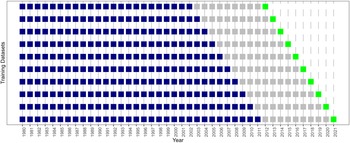
We perform out-of-sample validation using rolling forecasts 10 years into the future with the following procedure. First, we train the model with data from 1980 to 2002 and predict the outcome for 2012. Second, the model is trained with data from 1980 to 2003 and the outcome for 2013 is predicted. We continue this process, each time extending the training period by one year and forecasting the next year until we reach the most recent available data in 2021. This results in ten different models, each providing a 10-year-ahead forecast. Figure 1 illustrates the out-of-sample validation procedure.
Time-series out-of-sample validation technique.

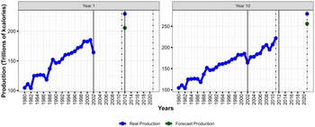
Figure 2 provides an alternative illustration of ten-year rolling forecasts generated for 2012 and 2021. The vertical lines indicate the end of the training data sets used to create the prediction. For example, when predicting production for 2012, we use a training data set from 1980 to 2002 to fit the model, then we predict area and yield in 2012. Finally, we calculate production in 2012 using the area and yield predictions as shown in green in Figure 2.
Illustration of time-series out-of-sample validation with preferred specification.
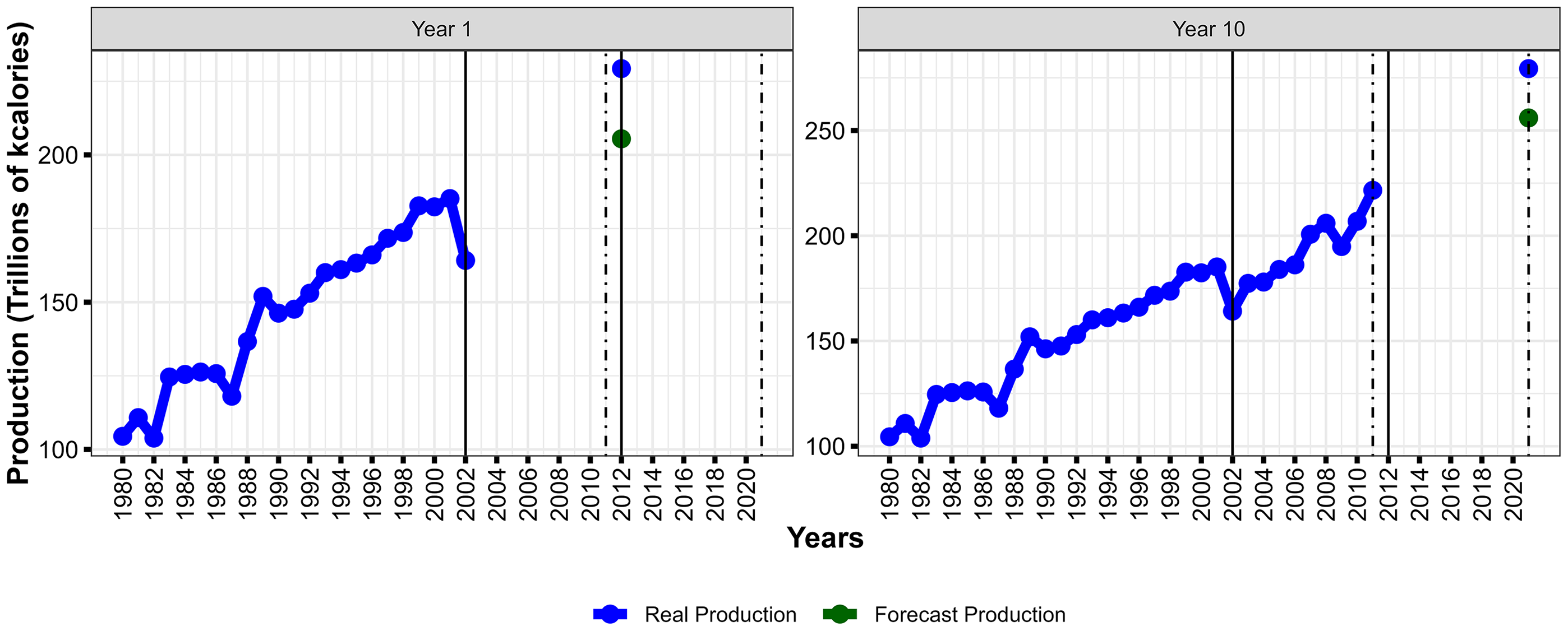
Out-of-sample prediction accuracy is shown by comparing the green point to the blue point. The graphs illustrate the challenge of forecasting production for 10 years in the future. For some countries, the trend in production in the training data up to 10 years prior to the prediction is leading in a different direction than actual production after the training period leading to an increase in forecasting errors. This reflects how unforeseen events can change the production trend at the country level.
Accuracy metrics
The prediction errors for each country in a given year (i.e., the difference between the out-of-sample forecast production values and the real production values in the test data set) are used to calculate the average Mean Absolute Error (MAE) in Equation (4), Mean Absolute Percentage Error (MAPE) in Equation (5), and Root Mean Square Error (RMSE) in Equation (6).
 $MAE = {{{1 \over N}\sum _{i = 1}^N\left( {{1 \over {10}}\sum _{t = 1}^{10}\left| {{{\hat Y}_{i,t}} - {Y_{i,t}}} \right|} \right)} \over {{1 \over N}\sum _{i = 1}^N\left( {{1 \over {10}}\sum _{t = 1}^{10}{Y_{i,t}}} \right)}},$
 $MAPE={1 \over N}{\sum }_{i=1}^{N}\left\{{1 \over 10}{\sum }_{t=1}^{10}\left[{| \hat{Y}_{i,t}-Y_{i,t}| \over Y_{i,t}}*100\right]\right\},$
 $RMSE={1 \over N}{\sum }_{i=1}^{N}\left\{\left[{1 \over 10}{\sum }_{t=1}^{10}{\left({\hat{Y}_{i,t}}-{Y_{i,t}}\right)^{2}}\right]^{1/2}\right\},$
where
 $\hat{{Y}}_{{{i,t}}}$
is the forecast value and Yit
is the real value of the predicted variable. To create a single accuracy measure across countries, we average the accuracy measures across 10 years and across all countries, where N is the total number of countries. We do not calculate a weighted average MAE or RMSE across countries because these metrics already implicitly include weighting – countries with larger production will tend to have larger errors and effectively receive more influence in the aggregate metric. We divide the MAE by average production so that the MAE is interpreted as the absolute error relative to average production.
Our preferred accuracy metric is the MAE because it leads to a specification that gives the smallest average prediction errors. Therefore, the preferred specification has the smallest MAE. These metrics are commonly used to evaluate forecasting models, but there is no clearly dominant metric since all have advantages and limitations. While we use MAE as the criteria to select the preferred model specification, we also show results for MAPE and RMSE. Different accuracy metrics indicate different preferred specifications. However, our main results are robust that the ARIMAX preferred specification provides the best forecast and that our method provides a significant improvement over the current GFA model.
We first estimate the models for area and yield separately and assess the model accuracy. The model specifications that perform best for area do not necessarily correspond with the model specifications that perform best for yield. Next, we selected the top ten models for predicting area using regression, the top ten models for predicting area using ARIMAX, and similarly select the top models for predicting yield. Finally, we calculate production using all combinations for regression and again for all combination for ARIMAX, resulting in 100 forecasts of production for regression specifications and 100 forecasts for ARIMAX specifications.
Using the selected model specification, we forecast production for ten years into the future (i.e., 2033) as would be the practice of the USDA GFA report. To create a production forecast in 2033, we do not attempt to forecast prices or weather in the future, so we use the most recent five-year average for each predictor as the assumed value for future years. Although we use recent historical weather data in the forecasts, including the weather predictors in the model can still improve forecast accuracy by improving the estimate of the trend by controlling for periods of good or bad weather in the training sample.
Results and discussion
The discussion of the results is composed of five sections. First, we discuss the forecast accuracy of the alternative models. Second, we describe the preferred model specification that provides the best forecast accuracy. Third, we discuss the forecasts of future production in 2023 and 2033 using the preferred specification. Fourth, we compare our forecast accuracy with the current GFA model. It is important to highlight that our main objective is to evaluate alternative methods to provide reliable grain supply forecasts for the long term and improve forecast accuracy. Therefore, we do not examine any causal inference relations between the predictor variables and production.
The information generated in this study contributes to assessing the domestic grain supply of the low- and middle-income countries. Forecasting food production is essential to identify potential supply shortages since we can determine which countries are more likely to have demand outpace supply. Also, this can be interpreted from an international trade angle since major grain exporter countries, like the U.S., can identify future demand for grain in the global markets.
Forecast accuracy of alternative models
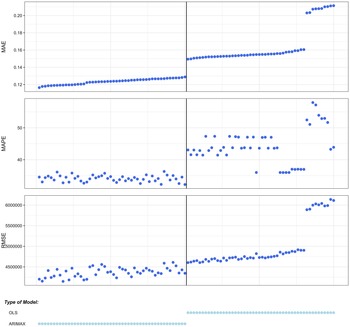
Figure 3 depicts the best combinations of area and yield models to predict production, specifically showing the Top 50 ARIMAX model combinations, and the Top 50 OLS model combinations. OLS models perform better than Poisson models and linear trends perform better than natural cubic splines, so we only show results using OLS with linear trends. Using the difference between the forecast and the real production values, we estimate the accuracy measures MAE, MAPE, and RMSE. A lower MAE, MAPE, and RMSE indicates better model forecast performance. We rank the models based on MAE, where the model with the lowest MAE is ranked first. The MAPE and RMSE are plotted using the MAE ranking in Figure 3.
Accuracy metrics of the Top 50 ARIMAX and OLS models.
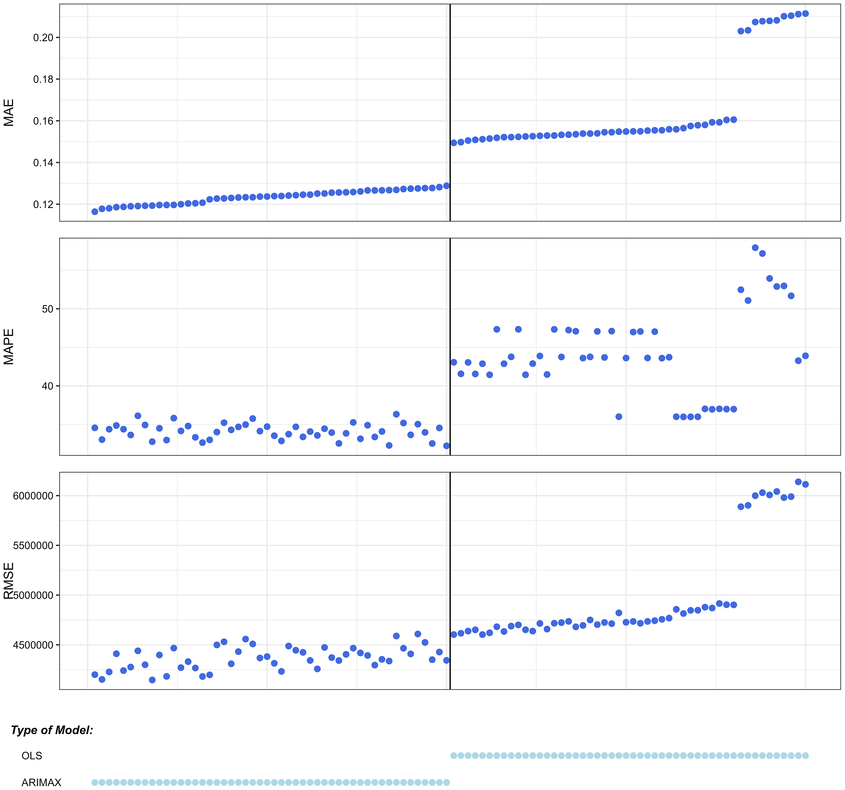
Figure 3 shows the ranking of the models and reveals that the Top 50 ARIMAX models span MAE values representing between 11% and 13% of average production, while the MAPE values range is 20–35%, and RMSE values range is 4,000,000–4,700,000. An MAE of 11% indicates that the average error of the 10-year production forecast was within 11% of average production. The model predicts well, especially in countries with large production, such as Cambodia, India, Indonesia, Malawi, Nigeria, and Pakistan.
While the figure does not explicitly show what aspects of the model specification improve prediction the most, we find that models with country-specific trends and country-fixed effects are especially important for prediction accuracy. For brevity, we report accuracy metrics for all of the area and yield models in Appendix A. The top ten models that forecast area have a MAE between 7.2% and 7.7% while the top ten models for yield have a MAE between 13.6% and 14.3%.
Preferred model specification
There are two preferred ARIMAX model specifications, one for yield and one for area. These models are used together to provide the lowest MAE of the forecast for production. The model specifications are:
 $\Delta Yiel{d_{i,t}}={\beta _i}\;Temperatur{e_{i,t}}+{\varphi _i}{\varepsilon _{i,t, - 1}}+{\alpha _i} +{\varepsilon _{i,t,}}$
 $\Delta Are{a_{i,t}}={\beta _i}\;Temperatur{e_{i,t}}+ {\beta _i}\;SpotPriceS{A_{i,t}}+{\alpha _i} + {\varepsilon _{i,t,}}$
where Yieldit and Areait represent Yield and Area, Temperatureit is average annual temperature, and SpotPriceSAit is the Spot Price using a Simple Average. Both models include country-specific coefficients and intercepts since the ARIMAX models are estimated separately for each country. The yield ARIMAX model has orders (0,1,1) which indicates the model is estimated using first differenced yield and with a Moving Average component of the yield. The area ARIMAX model has orders (0,1,0), implying differencing but no Autoregressive or Moving Average components. Note that the two preferred specifications both include differencing with an intercept, this indicates that the models implicitly include country-specific linear trends for area and yield. A lagged dependent variable for area is accounted for during the model selection process in order to reflect adjustments in expanding the growing area. A model that includes a lagged dependent variable with ARIMAX order (1,1,0) is the 5th best model for predicting area, but it is not the best model based on the accuracy measure (Figure A1 in the Supplementary Appendix).
We also considered forecasting production directly with a single time series rather than with separate forecasts for area and yield. The forecast performance of the best model to forecast production directly (MAE = 11.1% and RMSE = 4,186,176) is similar to the best model to forecast production using area and yield separately (MAE = 11.8% and RMSE = 4,152,450). The prediction intervals of our predictions were also similar using either method. Since forecasting production directly using a single time series does not substantially improve the forecast or prediction intervals, we prefer the method of forecasting area and yield separately because of the additional details that area and yield separately provide about production that are commonly reported. Another advantage of forecasting area and yield separately is that it allows for individual assessment of these two variables for any further analysis.
Forecasts with preferred model specification
In addition to improved forecast accuracy, additional extensions from the current modeling work are worth noting. Our results include prediction intervals for the forecasts. Adjemian et al. (Reference Adjemian, Bruno and Robe2020) highlight that distributional, interval and probabilistic forecasts offer valuable insights into the uncertainty surrounding predictions, providing a more comprehensive understanding of potential outcomes. The prediction intervals are obtained using the “forecast” package in R. The intervals are constructed under the assumption of normally distributed forecast errors. These values show and reflect the uncertainty arising from future shocks, as well as the dynamic structure of the ARIMAX models. The lower and upper bounds correspond to the 95% prediction intervals, conditional on observed exogenous variables (Hyndman and Khandakar Reference Hyndman and Khandakar2008; Hyndman et al. Reference Hyndman, Athanasopoulos, Bergmeir, Caceres, Chhay, O’Hara-Wild, Petropoulos, Razbash, Wang and Yasmeen2020).
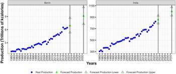
Figure 4 shows the forecasts and 95 percent prediction intervals for the forecasts for 2023 and 2033 production based on the preferred model specification to predict production for two example countries, Benin and India.Footnote 1 We train the models with all data from 1980 to 2021 to create the forecasts and intervals. Note that production is predicted for 2023 since 2023 production data were unavailable at the time of this analysis.
Illustration of 1 and 10-year production forecasts for Benin and India with prediction intervals.
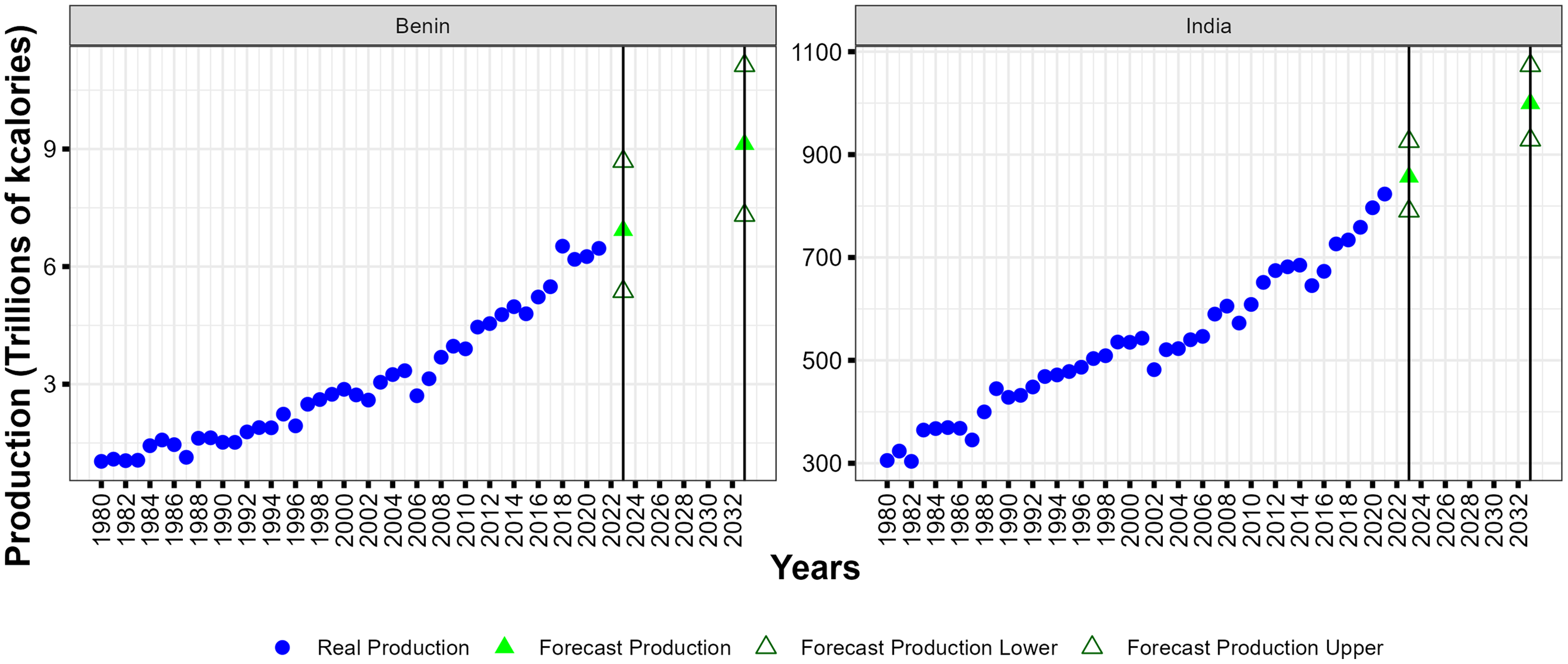
Actual production in the historical data is indicated in blue, the point forecasts for 2023 and 2033 are indicated with solid green, and prediction intervals are indicated with outlined green in Figure 4. The forecasts for 2023 and 2033 assume average prices and weather from the most recent five-year observed period. The 2023 forecast values shown in Figure 4 are only shown for the purpose of demonstrating how a model trained for long-term forecasting performs in a short-term context; no additional assessment is conducted on these forecast points.
Comparison with the GFA model
When comparing the performance of the existing GFA model and our preferred model specification, there are some data and modeling points to highlight. As discussed in the introduction section, yield is determined by inputs’ returns, technological advancements, and country-specific variables, while area depends on past area, expected crop and fertilizer prices, and a time trend (Zereyesus et al. Reference Zereyesus, Cardell, Valdes, Ajewole, Zeng, Beckman, Ivanic, Hashad, Jelliffe and Kee2022b). In the current paper, a broad range of regression model specifications for both yield and area are explored, including different predictor variables, pooling methods, fixed effects, functional forms, trend structures, and ARIMAX models. Another difference is that the existing GFA aggregates yield in metric tons per hectare.
The general specification to estimate the existing GFA model for yield employs the following econometric regression:
 $Yiel{d_{it}} = {\beta _{1,r}}t + {\beta _{2,r}}MA2{\mathop{\rm Re}\nolimits} v\_Fer{t_{i,t}}+{\beta _{3,r}}\;MA5{\mathop{\rm Re}\nolimits} v\_Fer{t_{i,t}}+ {\alpha _i} +{\varepsilon _{i,t,}},$
where Yieldit denotes the yield (millions of kcal per Hectare), αi are country fixed effects, and ϵi,t are residuals. The subscript i denotes each country, t denotes a year, and r denotes the region/subregion. Note that the coefficients on the trend and variables are specific to each subregion rather than each country. The variable MA2Rev_Ferti,t and MA5Rev_Ferti,t denote 2 year and 5 year lagged moving averages of the grain yield ratios to provide the short- to medium-term dynamics of return to yield after accounting for input costs as shown in the following equation:
 $MA2Rev\_ Fert_{i,t}={1 \over 2}{\sum }_{\tau =1}^{2}\left({\textit{DGrainP}_{i,t-\tau } \over \textit{DFertP}_{i,t-\tau }}*\textit{Yield}_{i,t-\tau }\right)$
where DGrainP is the domestic grain price and DFertP is the domestic fertilizer price. The variable MA5Rev_Ferti,t is calculated in a similar way, but using a lagged 5-year moving average. To estimate the existing GFA model for area we estimate the following regression:
 $Are{a_{i,t}} ={\beta _{1,r}}t +{\beta _{2,r}}Are{a_{i,t - 1}}+ {\beta _{3,r}}\;DGrain{P_{i,t}} +{\beta _{4,r}}\;DFert{P_{i,t}} +{\alpha _i} +{\varepsilon _{i,t,}}$
where Areai,t denotes the growing area (Hectares). For more information about the current GFA model, see Zereyesus et al. (Reference Zereyesus, Cardell, Valdes, Ajewole, Zeng, Beckman, Ivanic, Hashad, Jelliffe and Kee2022b).
To evaluate model performances and forecast accuracy, we use our out-of-sample validation. To overcome data restrictions due to the inclusion of 2-year and 5-year moving average, the training data starts from 1985. Additionally, only 65 countries are used for comparison because of a lack of data for some countries.Footnote 2
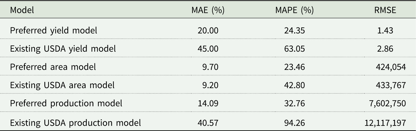
Using a data set with the same time frame and countries, we estimate the models with both the existing GFA model specification and our preferred model specification. We forecast yield and area using out-of-sample validation to obtain accuracy metrics (MAE, MAPE, and RMSE) for each model. As shown in Table 2, our selected model specification for yield demonstrates substantially better MAE, MAPE, and RMSE values compared to the existing GFA model specification.Footnote 3 Specifically, our preferred model specification reduces the 10-year forecast errors for yield by more than half in terms of MAE. For the area forecast, the MAE and RMSE are similar in magnitude to the existing GFA specification.Footnote 4 This is not surprising since the growing area tends to be more stable than yield so our specification does not offer a substantial improvement for the growing area. But overall, Table 2 demonstrates that our preferred model specification is a substantial improvement over the existing GFA model due to the improvement in the yield forecast.
Accuracy measures of preferred model and existing GFA model (65 countries from 1985 to 2021)
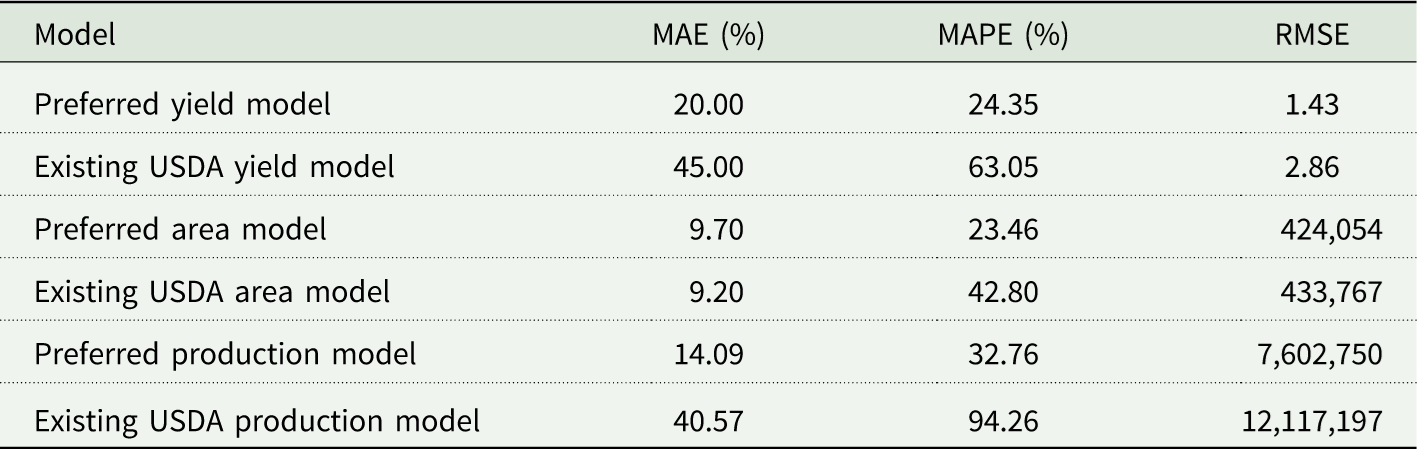
Table 2. Long description
The table has four columns Model, Mean Absolute Error (MAE), Mean Absolute Percentage Error (MAPE), and Root Mean Squared Error (RMSE). IT displays the accuracy measures of six models, three of these models are the preferred model (yield, area and production) and the other three models are the ucrrenct USDA models (yield, area and production)
Note: The accuracy measures are average across countries when predicting yield 10 years into the future.
Conclusion
This study evaluates alternative methods to provide reliable long-term forecasts of grain supply. Our study uses aggregated data at the country level and includes variables to capture and incorporate the heterogeneous conditions of each country and, consequently, to increase the forecast accuracy of grain supply models. The data set to train the models spans from 1980 until 2021 and includes 78 countries. We assess the accuracy of all models in this study using an out-of-sample validation methodology that accounts for the time-series nature of the data and the challenges of long-term forecasting. The preferred model specification is selected based on the MAE.
There are a few limitations of our empirical study worth noting. First, the preferred model specification will vary according to which accuracy measure is used as a criteria selection since the decision depends on the specific objectives of the forecast. Second, our models do not include any variables to capture policy changes affecting each country’s supply. Third, while we currently utilize the average temperature and precipitation data from the past five years, future research could enhance the forecasts by incorporating weather change projections.
Furthermore, changes in trade policy at the national or international level are an important source of forecasting inaccuracy (Clements and Hendry Reference Clements and Hendry2006; Hendry Reference Hendry2000; Koo and Seo Reference Koo and Seo2015; Stock and Watson Reference Stock and Watson1996). Adjustments in production and trade patterns, particularly in low- and middle-income countries, may be induced by changes in policy and may not be fully captured by historic production data and the variables considered in our methodology. While our approach relies on observed historical relationships, we recognize this limitation and the fact that forecasts should be interpreted with caution in the presence of unexpected structural changes.
While there are limitations in our work, we also show that our approach makes significant improvements in the accuracy of the 10-year forecast compared to existing methods. Improved forecasts for grain production (in caloric terms) are important for an accurate assessment of the future landscape of food security and international trade. In its GFA report, USDA subtracts its projections of supply from the projection of demand across 83 countries to calculate the IASR. The IASR identifies countries where demand growth is expected to outpace supply growth. These are countries where there will be a projected increase in grain demand which may lead to an increase in imports or a need for food aid. The projected disparity between demand and supply in certain countries offers significant market opportunities for exporters. While USDA does not currently utilize a partial equilibrium model in the GFA report, the forecasts of production that we generate could be used to calculate projected shifts in supply that could feed into partial equilibrium models to model future market conditions as well.
The results reveal four ways to improve forecast accuracy. First, the country-specific coefficients increase the forecast accuracy. Pooled coefficients reduce the number of parameters that must be estimated, while country-specific coefficients allow the model to capture more heterogeneity. Second, linear trends provide higher forecast accuracy than non-linear trends. Third, the best model specifications include weather variables such as temperature. Fourth, ARIMAX models with exogenous variables show higher accuracy than OLS models.
ARIMAX models, including fewer variables as predictors, show lower MAE values, implying that simpler models have higher accuracy for long-term forecasting. The lowest MAE achieved across all the models developed is 11.6%, which can be interpreted as an indicator of potential for further improvement of these types of long-term forecasting models. We consider this percentage acceptable given our study’s context, which focuses on long-term projections with aggregate data. To draw more precise conclusions, it would be necessary to fit forecasting models using higher-frequency data. This would allow for capturing, controlling, and incorporating local conditions within each country, enabling more detailed and specific insights.
Supplementary material
The supplementary material for this article can be found at https://doi.org/10.1017/age.2026.10040.
Data availability statement
The data used for this study are primarily from the USDA Foreign Agricultural Service Production, Supply, and Distribution (PSD). Data were also collected from the Chicago Board of Trade, World Bank Food and Agriculture Organization of the United Nations’s Global Information and Early Warning System (GIEWS), and the Climatic Research Unit (CRU) at the University of East Anglia. All data used are publicly available. The authors are willing to share the data sets used with anyone interested.
Funding statement
This research was funded by the U.S. Department of Agriculture, Economic Research Services (Cooperative Agreement 58-3000-1-0057).
Competing interests
Walter Ac-Pangan, Nathan P. Hendricks, Yacob Abrehe Zereyesus, and Jennifer Kee declare none.
Disclaimer
The findings and conclusions in this publication are those of the authors and should not be construed to represent any official USDA or U.S Government determination or policy.


 Open access

