





Impact statement
When validating synthetic turbulence time series generated by data-driven models, assessments typically rely on statistical moments up to the second order. However, such measures alone are insufficient to determine whether temporal memory and the underlying pairwise dependencies between coupled time series are faithfully preserved. This work demonstrates the practical importance of a set of linear and information-theoretic interaction measures for evaluating pairwise relationships in turbulence time series. The measures are applied to velocity time series extracted from a turbulent channel flow simulation and to their synthetic counterparts generated by a high-order vector autoregressive model. By comparing these measures between simulation and synthetic data, and examining how their directional patterns are consistent with turbulence physics, the study highlights their value as complementary validation tools for data-driven turbulence time-series generation.
1. Introduction
Turbulent flows are complex multiscale systems in which a wide range of spatio-temporal structures interact through various physical mechanisms (Jiménez, Reference Jiménez2018; Jiménez, Reference Jiménez2025; Massaro and Hussain, Reference Massaro and Hussain2026). The state variables, such as velocity, pressure, and their derivative quantities, are interconnected in both space and time. These dependencies are encoded in high-dimensional joint probability distributions, whose exact forms are practically unobservable. Typically, we obtain samples drawn from these underlying distributions through experiments, scale-resolving simulations, and more recently, data-driven models. The degree to which the resulting data preserve the properties of the true physics depends on their level of contamination by error and uncertainty originating from various sources. In practice, we work with turbulence time series, that is, discrete samples of continuous flow quantities recorded at a finite set of timestamps. Several studies have provided strong evidence that the marginal distributions of turbulence time series are typically non-Gaussian, often skewed, heavy-tailed, or intermittent (Kovasznay et al., Reference Kovasznay, Kibens and Blackwelder1970; Castaing et al., Reference Castaing, Gagne and Hopfinger1990; Jiménez, Reference Jiménez1998). This non-Gaussianity does not, however, pose a fundamental issue for most analyses in practice, as we are often interested in low-order turbulence statistics, such as mean velocity and Reynolds stresses. These quantities of interest have well-defined finite values, despite being affected by sampling uncertainty due to the finite size of time series (Oliver et al., Reference Oliver, Malaya, Ulerich and Moser2014; Russo and Luchini, Reference Russo and Luchini2017; Rezaeiravesh et al., Reference Rezaeiravesh, Xavier, Vinuesa, Yao, Hussain and Schlatter2022; Xavier et al., Reference Xavier, Rezaeiravesh and Schlatter2024). In contrast, what is challenging is how to characterise intrinsic interactions among multivariate time series recorded at different spatial locations within a turbulent flow. Linear interactions are typically quantified using statistical measures such as correlation, autocorrelation, and cross-covariance functions, that is, second-order statistics. In practice, these can be estimated accurately for weakly statistically stationary time series (or after being converted to that), see, for example, Wei (Reference Wei2006). For quantifying both linear and non-linear interactions, and for performing detailed structure analysis of turbulence time series (stationarity is not needed), we can employ information-theoretic measures (Cover and Thomas, Reference Cover and Thomas2001; Kantz and Schreiber, Reference Kantz and Schreiber2003), such as Shannon entropy (Shannon, Reference Shannon1948), mutual information (Fraser and Swinney, Reference Fraser and Swinney1986), and transfer entropy (Schreiber, Reference Schreiber2000).
The central objective of this study is to establish a rigorous validation framework for synthetic turbulence time series based on pairwise interaction measures. While designed for synthetic data, this approach is applicable to time series generated by predictive models when the forecast horizon is sufficiently long. Rather than relying solely on marginal or second-order statistics, the framework evaluates whether synthetic data preserve both linear and information-theoretic dependencies present in the reference turbulence data. In particular, we employ velocity time series obtained from a computational fluid dynamics (CFD) simulation as the reference (ground truth) and for training a linear vector autoregressive (VAR) model. The VAR model serves as a baseline benchmark to demonstrate the framework, but it can be replaced by other data-driven models, examples of which are cited below. This objective is both timely and novel, given the recent expansion of data-driven models for forecasting and synthesising turbulence time series, and the pressing need for more thorough validation measures. Indeed, outside of turbulence research, comprehensive assessment of the quality of synthetic time series has recently gained attention; see, for example, Bahrpeyma et al. (Reference Bahrpeyma, Roantree, Cappellari, Scriney and McCarren2021), Stenger et al. (Reference Stenger, Bauer, Prantl, Leppich, Hudson, Chard, Foster and Kounev2024).
The generation of inflow conditions for scale-resolving simulations is one of the most important applications of synthetic turbulence time-series generation; see, for example, the review by Wu (Reference Wu2017). In recent years, several deep learning models have been utilised for this purpose, including an autoencoder-type convolutional neural network with a multilayer perceptron (Fukami et al., Reference Fukami, Nabae, Kawai and Fukagata2019), generative adversarial networks (Kim and Lee, Reference Kim and Lee2020), a recurrent neural network (RNN) with LSTM (long short-term memory) (Yousif et al., Reference Yousif, Yu and Lim2022), a combination of transformer and generative models (Yousif et al., Reference Yousif, Zhang, Yu, Vinuesa and Lim2023), and diffusion models (Li et al., Reference Li, Biferale, Bonaccorso, Scarpolini and Buzzicotti2024; Liu et al., Reference Liu, Parikh, Fan, Du, Wang, Chen and Wang2025). Similarly, some of the main approaches for predicting turbulence time series for canonical wall-bounded turbulence include RNN-LSTM (Nakamura et al., Reference Nakamura, Fukami, Hasegawa, Nabae and Fukagata2021; Matsubara et al., Reference Matsubara, Mitsuishi, Iwamoto and Murata2023), transformers (Drikakis et al., Reference Drikakis, Kokkinakis, Fung and Spottswood2024), and echo state network (Racca et al., Reference Racca, Doan and Magri2023). Alternatively, statistical (mainly autoregression) and spectral approaches have been used for synthesising turbulence time-series, see, for example, (Klein et al., Reference Klein, Sadiki and Janicka2003; Basu et al., Reference Basu, Foufoula-Georgiou and Porté-Agel2004; Castro and Paz, Reference Castro and Paz2013; Patruno and Ricci, Reference Patruno and Ricci2018; Gallego-Castillo et al., Reference Gallego-Castillo, Elagamy, Cuerva-Tejero, Lopez-Garcia and Avila2024; Xavier et al., Reference Xavier, Rezaeiravesh and Schlatter2024). These models typically impose spatio-temporal connectivities when constructing the model to preserve time-delayed dependence to an extent. In particular, Stanly et al. (Reference Stanly, Du, Xavier, Perez, Mukha, Markidis, Rezaeiravesh and Schlatter2024) used a VAR model to synthesise the evolution of the temporal coefficients of the proper orthogonal decomposition in a boundary layer flow. The use of synthetic data at the inflow of another simulation resulted in achieving physical turbulence in a short adaptation length. In the present study, the same linear VAR model is used as a benchmark generator of synthetic turbulence time series from channel-flow data, allowing us to assess the extent to which linear and information-theoretic interaction structures are preserved.
Application of the information-theoretic measures (Shannon, Reference Shannon1948; Cover and Thomas, Reference Cover and Thomas2001; Kantz and Schreiber Reference Kantz and Schreiber2003) to turbulence has received considerable attention in recent years. Examples include the use of transfer entropy for identifying causality in turbulence structure in different parts of boundary layers (Lozano-Durán et al., Reference Lozano-Durán, Bae and Encinar2019; Massaro et al., Reference Massaro, Rezaeiravesh and Schlatter2026; Zhang et al., Reference Zhang, Zhu, Wang and Hu2025), flow control and subgrid-scale modelling (Lozano-Durán and Arranz, Reference Lozano-Durán and Arranz2022), and driving computational algorithms (Massaro et al., Reference Massaro, Rezaeiravesh and Schlatter2023). To ensure the reliability of the information-theoretic analyses, the present study examines the sensitivity of the numerical estimates to estimator parameters and embedding choices, and employs surrogate-based significance tests following Pinto et al. (Reference Pinto, Lazic, Antonacci, Pernice, Gu, Barà, Faes and Rocha2024).
The remainder of this paper is organised as follows. Section 2 introduces the methodology, including the turbulence dataset, the VAR modelling approach, and the interaction measures. Section 3 presents the analysis of the linear and non-linear measures applied to the turbulent channel-flow data and the corresponding VAR-based synthetic time series.
2. Methodology
2.1. Turbulence time series data
The CFD-based time series data in this study are obtained from the wall-resolving simulation of a turbulent channel flow at a friction-based Reynolds number
$ {\operatorname{Re}}_{\tau }=300 $
 (Figure 1a). This Reynolds number is defined as
$ {\operatorname{Re}}_{\tau }={u}_{\tau}\delta /\nu $
 where
$ {u}_{\tau } $
 is the mean wall friction velocity,
$ \delta $
 is the channel half-height, and
$ \nu $
 is the kinematic viscosity. As detailed in Rezaeiravesh et al. (Reference Rezaeiravesh, Vinuesa and Schlatter2021), the simulation has been performed by the open-source spectral-element solver, Nek5000 (Fischer et al., Reference Fischer, Lottes and Kerkemeier2008). The computational mesh consists of fully structured elements with uniform spacing in the streamwise (
$ x $
 ) and spanwise (
$ z $
 ) directions and compression towards the walls. Each element contains
$ {\left({N}_p+1\right)}^3 $
 Gauss–Lobatto–Legendre points (where
$ {N}_p=7 $
 is the polynomial order), at which the discretised Navier–Stokes equations are solved. The first off-wall grid point is located at
$ {y}^{+}=0.55 $
 , where
$ {y}^{+}=\left(y/\delta \right){\operatorname{Re}}_{\tau } $
 denotes the wall-normal distance in wall units. Periodic conditions are applied in the streamwise and spanwise directions, where the average spacing between grid points is approximately
$ 20 $
 and
$ 10 $
 wall-units, respectively. After discarding the initial transient, a total of 104,377 time samples are collected for the velocity at 64 points in the wall-normal direction,
$ y $
 , across
$ \delta $
 . The velocity values are averaged over the wall-parallel (
$ xz $
 ) planes and sampled at constant time intervals
$ 0.008\delta /{U}_b $
 , equivalent to
$ 0.15\delta /{u}_{\tau } $
 , where
$ {U}_b $
 is the bulk velocity.
(a) A snapshot of the streamwise velocity component,
$ u $
 , in the turbulent channel flow considered in this study. The yellow markers schematically indicate the sampling locations in the wall-normal direction,
$ y $
 . At each location, the streamwise velocity averaged over the
$ xz $
 -plane is sampled at a fixed rate to generate a simulation time series. (b) Example time series sampled at
$ {y}^{+}=11 $
 (top) and
$ {y}^{+}=180 $
 (bottom). The black lines denote the simulation data, and the coloured lines denote three realisations generated by the VAR model fitted to those data.

Figure 1. Long description
Panel a is a 3 D volume rendering of streamwise velocity u. At the bottom-left corner, a coordinate system shows y pointing upward, x pointing right, and z pointing into the depth. The top surface is labeled Wall. A horizontal dash-dotted line marks the Centreline, with the distance from the wall to the centreline labeled delta. A vertical line of yellow dots indicates sampling locations along the y-axis. The flow field is colored in shades of blue and white, representing turbulent fluctuations.
Panel b contains two vertically stacked line graphs. Both share an x-axis labeled Time index ranging from 0 to 10000. The y-axis for both is u all over bulk velocity.
- The top graph represents y plus equals 11, with y-axis values from 0.46 to 0.50.
- The bottom graph represents y plus equals 180, with y-axis values from 1.085 to 1.095.
In both graphs, a thick black line represents the original simulation data, showing high-frequency oscillations. Three thinner colored lines in blue, green, and red represent different realizations generated by a VAR model, which closely track the stochastic nature and amplitude of the black simulation line.
2.2. Vector autoregression (VAR)
Consider a set of
$ K $
 time series
$ \mathbf{X}=\left[{X}^{(1)},{X}^{(2)},\cdots, {X}^{(K)}\right] $
 belonging to the same system with some underlying interactions and dependencies. A
$ K $
 -variate VAR model of order
$ p $
 can be used as a linear approximation to the dynamical systems described by the time series (Lütkepohl, Reference Lütkepohl2005):

Here,
$ {\mathbf{x}}_t={\left[{x}_t^{(1)},{x}_t^{(2)},\cdots, {x}_t^{(K)}\right]}^T $
 ,
$ {\mathbf{A}}_{\mathrm{\ell}} $
 is a
$ K\times K $
 coefficient matrix at lag
$ \mathrm{\ell} $
 , and the noise vector (innovation process)
$ {\boldsymbol{\varepsilon}}_t $
 has a multivariate Gaussian distribution with covariance matrix
$ {\mathbf{C}}_{\boldsymbol{\varepsilon}} $
 . Given a set of joint samples of length
$ n $
 for the time series, the coefficient and noise covariance matrices can be estimated using Least Squares (LSE), Maximum Likelihood (MLE), or Bayesian methods. After construction, the VAR(
$ p $
 ) model, as a stochastic process, can be used to synthesise samples for
$ \mathbf{X} $
 of any length, with a temporal resolution identical to the training data.
2.3. Interaction measures
In general, there can be various measures of linear and non-linear interactions between each two components of a
$ K $
 -variate time series. The most standard measure of the statistical linear dependence between two time series
$ X $
 and
$ Y $
 is the cross-covariance function (CCF), which measures both concurrent and time-shifted covariances between the time series:

where
$ \tau >0 $
 is the time shift (lead/lag),
$ \unicode{x1D53C}\left[\cdot \right] $
 denotes the expected value, and
$ \mu $
 is the mean of a time series. The CCF is asymmetric, meaning that its value changes depending on whether
$ X $
 leading or lagging
$ Y $
 . The only symmetry is
$ {\gamma}_{XY}\left(\pm \tau \right)={\gamma}_{YX}\left(\mp \tau \right) $
 . For
$ \tau =0 $
 , the standard cross-covariance between
$ {x}_t $
 and
$ {y}_t $
 is recovered, which is not necessarily the maximum value across all possible values of
$ \tau $
 . In studies of turbulent flows,
$ {\gamma}_{XY}(0) $
 is widely used since, when
$ X $
 and
$ Y $
 are velocity components, it represents a component of the Reynolds stress tensor. If both time series are identical, then the CCF (2) is reduced to an autocovariance function to measure how each sample in a time series covaries with its own past. Normalising the autocovariance function with the variance of the time series, the autocorrelation function (ACF) is derived:

that is, symmetric. In practice, where there is only one realisation of a turbulent flow, the expectation in covariances is replaced by a sample-mean estimator. As a result, the CCF and ACF are intrinsically oscillatory at high time lags/leads
$ \tau $
 .
Information theory (Cover and Thomas, Reference Cover and Thomas2001; Kantz and Schreiber, Reference Kantz and Schreiber2003) provides a set of measures for quantifying both linear and non-linear interactions between time series. A fundamental quantity is the Shannon entropy (Shannon, Reference Shannon1948), which provides a rigorous measure of the uncertainty or information content of a random variable. For
$ X $
 , a continuous random variable (with discrete values), the differential entropy is defined as,

where
$ p(X) $
 is the probability density function (PDF) of
$ X $
 . Building on entropy, various measures of interactions between multiple random variables or time series can be obtained. Shannon (Reference Shannon1948) proposed mutual information (MI) to measure the amount of shared information between two or more random variables. In connection with dynamical systems, the time-delayed MI was proposed by Fraser and Swinney (Reference Fraser and Swinney1986), which for two time series
$ X $
 and
$ Y $
 is defined as:

where
$ \tau \ge 0 $
 is the time delay and
$ p\left({x}_t,{y}_{t-\tau}\right) $
 is the joint PDF of
$ {x}_t $
 and the delayed
$ {y}_t $
 . This measures how much knowledge about the past of
$ Y $
 , that is,
$ {y}_{t-\tau } $
 , reduces uncertainty about the current state of
$ X $
 . Therefore, it is a measure of statistical dependence between
$ X $
 and
$ Y $
 considering both linear and non-linear effects in contrast to CCF (2). Clearly,
$ {I}_{XY}\left(\tau \right)\ne {I}_{YX}\left(\tau \right) $
 , meaning the time-delayed mutual information is, in general, asymmetric in time. However, because mutual information is symmetric under interchange of the two variables in the joint PDF in Equation (5)it does not, by itself, capture the directionality of information transfer. To obtain this, a conditional PDF was used by Schreiber (Reference Schreiber2000) who defined transfer entropy (TE) from
$ X $
 to
$ Y $
 as,

Given samples
$ {x}_t $
 and
$ {y}_t $
 from a single realisation, the time-delay embedding is used to reconstruct multi-dimensional state-space:

where
$ m\ge 1 $
 and
$ \tau \ge 1 $
 are the embedding dimension and embedding delay, respectively. The time-delay embedding used here follows the practical reconstruction procedure introduced by Packard et al. (Reference Packard, Crutchfield, Farmer and Shaw1980), and is theoretically motivated by Takens’ embedding theorem (Takens, Reference Takens1981), which establishes conditions under which the attractor of a dynamical system can be reconstructed from delayed observations of a scalar time series. Note that in the original definition by Schreiber (Reference Schreiber2000), each time series can have a different
$ m $
 , but in this study they are assumed to be the same. The choice of
$ m $
 and
$ \tau $
 can have a significant influence on the value of the estimated TE; see Tan et al. (Reference Tan, Algar, Corrêa, Small, Stemler and Walker2023), Wallot and Mønster (Reference Wallot and Mønster2018), and also the discussion in Section 3. According to Equation (6),
$ {\mathrm{TE}}_{X\to Y} $
 quantifies how much additional information is learned from the past of
$ X $
 in addition to what is already known from the past of
$ Y $
 , for predicting a future state of
$ Y $
 . This interpretation is directly reflected in the conditional PDFs in Equation (6). Therefore,
$ {\mathrm{TE}}_{X\to Y} $
 serves as a measure of statistical causality, indicating the extent to which
$ X $
 influences
$ Y $
 . However, the present bivariate TE is evaluated for the pair X and Y in isolation from the remaining time series. As a result, its causal interpretation is limited, since potential common drivers, redundant effects, and other multivariate dependencies are not taken into account. Nevertheless, it remains suitable for the purpose of the present study, that is, quantifying pairwise interactions between time series. In addition, compared with multivariate TE, the estimation of bivariate TE is more robust for a given dataset because of the lower dimensionality of the embedding space. Obviously,
$ {\mathrm{TE}}_{X\to Y}\left(m,\tau \right)\ne {\mathrm{TE}}_{Y\to X}\left(m,\tau \right) $
 motivating the definition of the net TE as
$ {\mathrm{TE}}_{X\to Y}-{\mathrm{TE}}_{Y\to X} $
 which indicates the dominant direction of information transfer in a time series pair.
Given a finite set of samples for two time series
$ X $
 and
$ Y $
 , computing MI and TE requires estimating various types of PDFs. The most basic approach is using binning to empirically estimate the PDFs, which, however, can be very sensitive to various parameters, for example, the bin size. The estimates can be improved using the Kernel Density Estimation (KDE) method that returns smooth PDFs. This can, however, lead to filtering some details. In general, the KDE method is sensitive to bandwidth selection and may struggle with high-dimensional data; see, for example, Lee et al. (Reference Lee, Nemati, Silva, Edwards, Butler and Malhotra2012), Zambom and Dias (Reference Zambom and Dias2013), and Appendix A. The most conventional method for estimating MI is based on
$ k $
 -nearest neighbour (KNN) distances, hereafter referred to as the KSG method after Kraskov et al. (Reference Kraskov, Stögbauer and Grassberger2004). We use their estimator for the mutual information that was derived based on an expansion of different Shannon entropies (Cover and Thomas, Reference Cover and Thomas2001). It reads as,

where
$ k $
 is the number of nearest neighbours,
$ \psi \left(\cdot \right) $
 is the digamma function,
$ n $
 is the length of the time series,
$ \left\langle \cdot \right\rangle $
 denotes an average over
$ n $
 , and
$ {n}_X(t) $
 specifies the number of
$ {x}_{t^{\prime }} $
 samples whose distance from
$ {x}_t $
 is less than a radius (computed in the method). The TE in Equation (6) can be written as a conditional time-delayed MI and expanded in terms of entropies (Frenzel and Pompe, Reference Frenzel and Pompe2007; Hlaváčková-Schindler et al., Reference Hlaváčková-Schindler, Paluš, Vejmelka and Bhattacharya2007):

Based on this, Frenzel and Pompe (Reference Frenzel and Pompe2007) extended the KSG estimator (Kraskov et al., Reference Kraskov, Stögbauer and Grassberger2004) to compute
$ {\mathrm{TE}}_{X\to Y} $
 from,

where
$ {n}_{y_t^m} $
 ,
$ {n}_{y_t{y}_t^m} $
 , and
$ {n}_{x_t^m{y}_t^m} $
 count the number of samples falling within a specific radius of the respective marginal space. Although the KSG estimators are non-parametric, their estimates can be affected by the choice of
$ k $
 . In general, smaller
$ k $
 values result in lower bias but more variance in the estimates (capturing local effects and letting the PDF vary over different regions), and vice versa (Stoļarovs et al., Reference Stoļarovs, Toosi, Yang, Massaro, Garcia, Yao, Mihajlović, Hussain, Rezaeiravesh and Schlatter2026). Gao et al. (Reference Gao, Oh and Viswanath2018) explained why KSG estimations are accurate for fixed values of
$ k $
 . Furthermore, there are methods to choose optimal
$ k $
 values to reduce the bias in the estimator, see, for example, Witter and Houghton (Reference Witter and Houghton2024). In this study, we select
$ k=10 $
 as a pragmatic intermediate value, rather than claiming it as an optimal choice across all time-series pairs. The sensitivity of the estimated information-theoretic measures to the choice of
$ k $
 is further detailed in Appendix A. Using the same value
$ k=10 $
 for both the simulation and synthetic time-series pairs is consistent with the main objective of the study, namely validation, although its potential impact on the physical interpretation of the results should be acknowledged.
3. Results and discussion
A set of
$ 22 $
 non-equispaced points (a subset of the original 64 points) in the wall-normal direction of the channel flow described in Section 2.1 is selected, at which time series of plane-averaged streamwise velocity are considered, see Figure 1a. The corresponding wall-normal locations span from
$ {y}^{+}=0.55 $
 (adjacent to the wall) to
$ {y}^{+}=298 $
 (the channel centre), with multiple sampling points located within the viscous sublayer, buffer layer, logarithmic layer, and wake region of the turbulent boundary layer (Pope, Reference Pope2000). The time series contain 10,437 samples, obtained by down-sampling the original CFD data by a factor of 10, resulting in a temporal resolution of
$ 0.08\delta /{U}_b $
 . The resulting 22 time series create 231 distinct interacting pairs, for which the interaction measures in Section 2.3 are evaluated using an in-house Python code. To reduce overall computational cost, a message-passing interface (MPI) parallelisation is implemented, where the computations associated with each pair of time series are assigned to a separate rank.
A VAR model of order
$ p=60 $
 is trained using the above 22-variate time series, employing the least-squares estimator available in statsmodels (Seabold and Perktold, Reference Seabold and Perktold2010). Example time series generated by the VAR model at two sampling locations are shown in Figure 1b. It is noteworthy that applying the Akaike Information Criterion (AIC) (Akaike, Reference Akaike1974) and the Bayesian Information Criterion (BIC) (Schwarz, Reference Schwarz1978) yields suitable VAR orders of
$ 20 $
 and 15, respectively. However, as the VAR model is used here for synthetic sample generation to reproduce the interaction structure of the time series, we adopt
$ p=60 $
 as a pragmatic choice to retain sufficiently long temporal memory. Importantly, repeating the analyses in the following sections with
$ p=30 $
 does not lead to any discernible change in the results. The only noticeable difference is that
$ p=60 $
 yields a slightly better agreement of the mean cross-covariance function with the simulation data at higher lags (see Figure 3).
Using the trained VAR model,
$ 50 $
 independent realisations of synthetic time series, each of length 10,437, are generated. The strategy in the subsequent analyses is to compare the empirical mean of the pairwise interaction measures obtained from the
$ 50 $
 synthetic realisations with the corresponding measures computed from the simulation data (ground truth) used for training of the VAR model. The ensemble of synthetic realisations also allows for estimating
$ 95\% $
 confidence intervals for the interaction measures between the VAR-generated time series.
3.1. Linear interactions
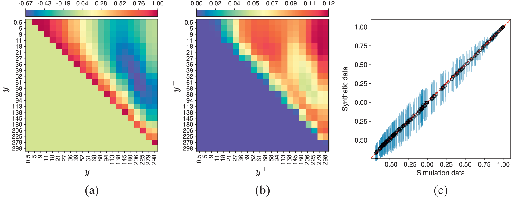
Figure 2a shows the matrix of mean correlation coefficients for the time series pairs obtained from the VAR model (the values between identical time series are excluded from all matrix plots). As expected, the time series show a high positive correlation with the neighbouring wall distances. For
$ {y}^{+}\lesssim 25 $
 (almost up to the end of the buffer layer), a high concurrent (i.e., no time-delay) linear dependency between time series is observed, as is known in the classical boundary layer theory, see, for example, Pope (Reference Pope2000). It is interesting to spot two regions of small/zero correlation encompassing pairs with highly negative correlations. In both regions, the time series up to
$ {y}^{+}\lesssim 27 $
 are involved, which show small/no linear correlation with the dynamics near the channel centre as well as with
$ 50\lesssim {y}^{+}\lesssim 80 $
 . As shown in Figure 2b, the same sets of interacting time series correspond to most of the high-uncertainty correlations of synthetic data. In contrast, for highly correlated pairs, the uncertainty in the correlation coefficient of the synthetic time series is low. As expected from a linear model, the VAR model perfectly preserves the correlation coefficient as compared to the ground truth, as inferred from the scatter plot in Figure 2c.
(a, b) Matrices of the mean and standard deviation of the correlation coefficient obtained from the VAR synthetic data, and (c) scatter plot of the correlation coefficient between the 231 time series pairs within the synthetic and simulation data. In (a, b), the
$ {y}^{+} $
 values of the 22 sampling points are shown on the axes. In (c), the bars present 95% confidence intervals around the mean values of the synthetic data, due to the stochastic nature of the VAR model. In each figure in this study, the colourbar limits are set to the minimum and maximum values of the corresponding dataset.

Figure 2. Long description
A three-panel layout labeled a, b, and c.
Panel a is a heatmap titled with a colorbar ranging from negative 0.67 to 1.00. Both the x and y axes are labeled y plus and feature 22 sampling points ranging from 0.5 to 298. The matrix shows a diagonal of high correlation (red) with varying patterns of positive (orange/yellow) and negative (blue/green) correlations in the upper right triangle, while the lower left triangle is a uniform light green.
Panel b is a heatmap showing the standard deviation, with a colorbar ranging from 0.00 to 0.12. The axes are identical to panel a. The upper right triangle shows higher standard deviation values (red and orange) concentrated towards the right edge, while the lower left triangle is a uniform dark purple representing zero.
Panel c is a scatter plot comparing Simulation data on the x-axis to Synthetic data on the y-axis, both ranging from negative 0.75 to 1.00. A series of black circular data points follows a tight linear 45-degree upward trend. Each point is overlaid with a vertical light blue bar representing a 95 percent confidence interval. A dashed red diagonal line serves as a reference for a perfect one-to-one correlation.
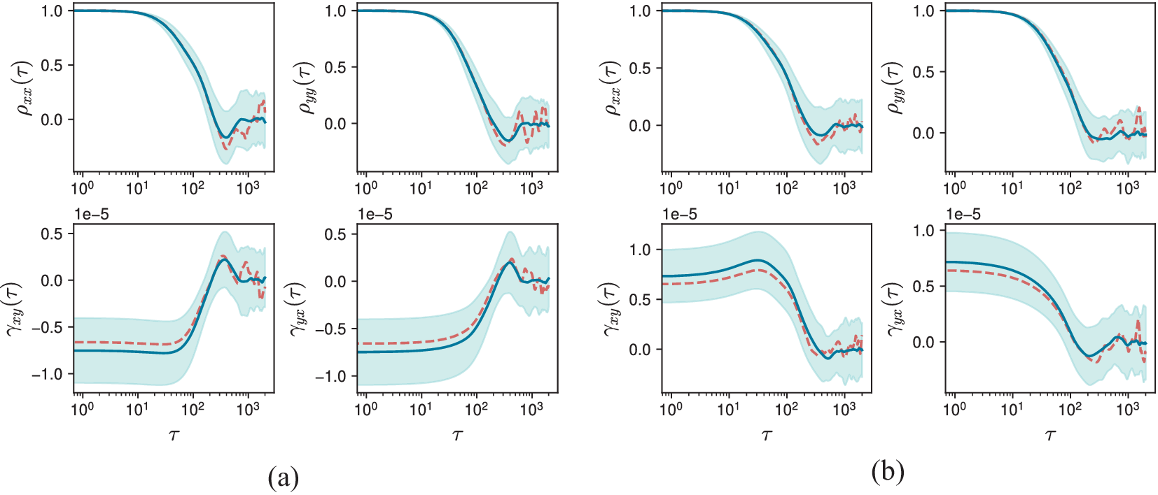
Next, we examine additional second-order linear measures that account for time-delayed dependencies, specifically the ACF and CCF. In Figure 3, these measures are evaluated for two pairs of time series with highly negative and positive correlation coefficients. The ACF is a measure of linear dependency of a time series with its own past, and indicates the time scale over which linear memory lasts. Similarly, the CCF measures how the past (or future) of a time series linearly covaries with the future (or past) of another time series. For the time series analysed here, the ACFs start from 1 and decay to zero at high lags, although they may show non-monotonic decay at higher lags. The latter can be an indication of a dominant time-periodic structure in the time series’ past. The time it takes for the ACF of a time series to reach zero can be taken as an integral time scale required to make samples uncorrelated to their past. As visible in Figure 3, such time can be significantly long, of the order of a few hundred time lags. Such long-lasting memories are, however, known in the turbulence community and, in practice, lead to slow convergence of turbulence statistics; see, for example, Oliver et al. (Reference Oliver, Malaya, Ulerich and Moser2014), Rezaeiravesh et al. (Reference Rezaeiravesh, Gscheidle, Peplinski, Garcke and Schlatter2025), Xavier et al. (Reference Xavier, Rezaeiravesh and Schlatter2024).
Linear time-delayed interactions between time series located at (a)
$ {y}^{+}=36,180 $
 and (b)
$ {y}^{+}=61,88 $
 . In each subplot, the top and bottom rows show the ACF and CCF versus time lag
$ \tau $
 , respectively. Dashed lines: simulation data, solid lines: mean of the synthetic data, and shaded area:
$ 95\% $
 confidence interval for the synthetic data.

Figure 3. Long description
The figure consists of two subplots, (a) and (b). Each subplot contains four graphs arranged in two rows and two columns. All graphs share a logarithmic x-axis representing time lag tau, ranging from 10 super 0 to 10 super 3.
In subplot (a), representing y plus equals 36 and 180:
* The top row shows A C F values rho sub x x and rho sub y y. Both curves start at 1.0, remain stable until tau equals 10 super 1, then show a steep sigmoidal decrease toward zero, followed by minor oscillations.
* The bottom row shows C C F values gamma sub x y and gamma sub y x. Both curves start at a negative value near minus 0.75 times 10 super minus 5, remain flat, then rise sharply around tau equals 10 super 2 to a peak near 0.25 before oscillating.
In subplot (b), representing y plus equals 61 and 88:
* The top row shows A C F values rho sub x x and rho sub y y, following a similar decay pattern to subplot (a), dropping from 1.0 to near zero after tau equals 10 super 1.
* The bottom row shows C C F values gamma sub x y and gamma sub y x. These curves start at positive values between 0.5 and 0.75 times 10 super minus 5, maintain a plateau, and then decrease toward zero after tau equals 10 super 2.
In all graphs, dashed red lines represent simulation data, solid blue lines represent the mean of synthetic data, and light blue shaded regions indicate the 95% confidence interval.
Depending on the time series pair, the plots of CCFs can exhibit more diverse patterns. For any pair, the zero-lag value satisfies
$ {\gamma}_{XY}(0)={\gamma}_{YX}(0) $
 , which represents the cross-covariance between the two concurrent time series. At higher lags, however, asymmetries in the CCF may arise. For instance, in Figure 3b, a “bump” is observed at higher
$ \tau $
 values for
$ {\gamma}_{XY}\left(\tau \right) $
 , suggesting the existence of event(s) in the past of
$ Y $
 that highly linearly covaries with the future of
$ X $
 (but not the other way around, in this specific case). This aligns with earlier observations by Massaro et al. (Reference Massaro, Rezaeiravesh and Schlatter2023). Across all considered time series pairs, the VAR model reliably reproduces the ACF and CCF, showing good agreement with simulation data. Note that due to the empirical average over the VAR realisations, the intrinsic oscillations in the ACF and CCF at high lags of the synthetic data exhibit lower amplitude than those observed in the simulation data. Furthermore, the empirical uncertainty in the ACF increases with
$ \tau $
 , with the highest values at non-physical oscillations around zero ACF. In contrast, for the CCF, the uncertainty in the VAR values is high across all lags, in addition to a small deviation between the mean CCF of VAR and the sample-estimated CCF of the simulation data. It is noteworthy that the Fourier transform of the ACF and CCF leads to power spectral and cross-spectral densities, respectively (see, e.g., Park, Reference Park2018), that are instrumental in turbulence studies. Therefore, the excellent agreement observed here between the linear time-delayed covariances of the VAR-synthetic and simulation time series is also expected to hold in the frequency domain.
3.2. Information-theoretic measures
The time-delayed mutual information (5) can measure the amount of shared information between a pair of time series. While
$ {I}_{XY}\left(\tau \right) $
 is comparable to the CCF
$ {\gamma}_{XY}\left(\tau \right) $
 , it can capture both linear and non-linear dependencies between
$ X $
 and
$ Y $
 (Shannon, Reference Shannon1948). The time-delayed MI has been previously evaluated for a few turbulent flows, see Arranz and Lozano-Durán (Reference Arranz and Lozano-Durán2024), Cerbus and Goldburg (Reference Cerbus and Goldburg2013), Granero-Belinchon (Reference Granero-Belinchon2018). For the present data, the time-delayed MI was found to be, in general, a decaying function of
$ \tau $
 (see, e.g., Figure 5a), where the decay rate could be regarded as the rate at which information (dependencies) between two time series is lost at different
$ \tau $
 . In particular, we are mainly interested in the maximum time-delayed MI, which is heuristically computed by searching over a set of candidate values of
$ \tau $
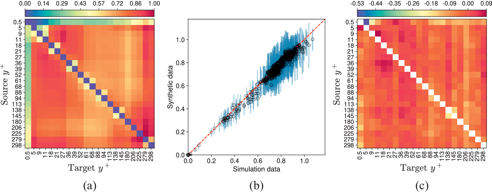
 . The motivation for this choice is that the lag at which the strongest time-delayed dependence occurs varies across interacting pairs, while the maximum of the time-delayed MI serves as a compact summary measure. Although this choice may be more sensitive to noise than MI evaluated at a prescribed lag, it avoids introducing an arbitrary common lag across all pairs and is applied consistently to both the simulation and VAR data. In Figure 4a, the mean value of this measure is shown for different pairs of time series synthesised by the VAR model. The vertical and horizontal axes show the
$ {y}^{+} $
 value of the source and target time series, respectively. The plot suggests a high level of symmetry in maximum TE, evident from the values on both sides of the main diagonal. In addition to high values of maximum MI between spatially close locations, a set of high values is observed below
$ {y}^{+}\approx 21 $
 . For the time series very close to the wall (at
$ {y}^{+}=0.5 $
 ), the maximum MI remains small when the
$ {y}^{+} $
 of the pair increases beyond
$ \approx 27 $
 . This is in contrast to the behaviour of the correlation coefficient in Figure 2a.
(a) Matrix of the mean maximum MI estimated from synthetic data, (b) scatter plot of the maximum MI obtained from the synthetic and simulation data, and (c) matrix of the normalised error (equation 11).

Figure 4. Long description
A three-panel scientific visualization.
Panel a is a heat map matrix titled Source y plus on the vertical axis and Target y plus on the horizontal axis. Values on both axes range from 0.5 to 298. A color scale at the top ranges from 0.00 to 3.25, transitioning from blue to yellow to red. The matrix shows a strong diagonal trend of high M I values, with the highest values appearing as dark purple and orange squares along the main diagonal against a teal background.
Panel b is a scatter plot comparing Simulation data on the x-axis to Synthetic data on the y-axis, both ranging from 0.0 to 3.5. A dashed red diagonal line represents a perfect one-to-one correlation. Data points, shown as black circles with light blue vertical error bars, are tightly clustered along this red line, indicating high accuracy between the two datasets.
Panel c is a heat map matrix of normalized error with the same Source y plus and Target y plus axes as panel a. The color scale at the top ranges from minus 0.09 to 0.25. The main diagonal is white, representing zero error. The surrounding cells show a variegated pattern of teal, yellow, and red, with higher error concentrations appearing in the lower-left and middle-right regions of the matrix.
According to the scatter plot in Figure 4b, the mean of the maximum MI obtained from the synthetic data agrees relatively well with those from the simulation data. Remarkably, this indicates that the PDFs in Equation (5) estimated from the VAR predictions closely approximate those of the simulation data, hence resulting in comparable values of the summation. The accuracy of the maximum MI predicted by the VAR data is further assessed in Figure 4c, via evaluating the following normalised error:

where the overbar stands for the empirical averaging over the repetitions of the VAR predictions. For most of the pairs, the error is positive, indicating over-prediction of time-delayed MI by the VAR synthesised data, which could be translated to spurious shared information. Additionally, the error plot is, to a large extent, asymmetric and shows that the highest errors more frequently occur when a time series at
$ {y}^{+}\ge 88 $
 interacts with a time series in the same region or very close to the wall.
Next, we consider bivariate TE as a measure of non-linear statistical causality between a pair of time series. A key to accurate estimation of TE for a dynamical system is constructing a valid time-delay embedding; see Equation (7). We consider multiple candidate values of the embedding dimension
$ m $
 to compute TE across several wall-normal locations. For high-order dynamical systems like turbulent flows, selecting the time delay
$ \tau $
 is non-trivial and critically affects the results, see Appendix B. To optimise
$ \tau $
 , several methods have been suggested in the literature for time series in various applications, see Wallot and Mønster (Reference Wallot and Mønster2018), Tan et al. (Reference Tan, Algar, Corrêa, Small, Stemler and Walker2023), and references therein. For chaotic dynamical systems, Fraser and Swinney (Reference Fraser and Swinney1986) showed choosing
$ \tau $
 based on the local minimum of
$ {I}_{XX}\left(\tau \right) $
 , the time-delayed MI of a time series with its own past, aka, auto-mutual information function (AMIF), can be a better option compared to the local minimum or first zero of the ACF of
$ X $
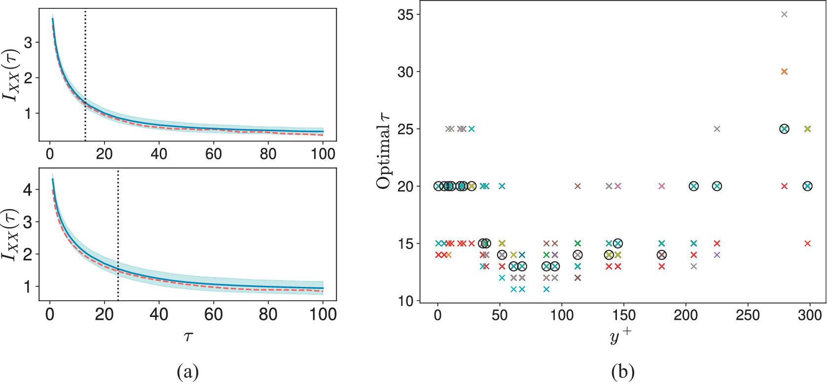
 . Further, relying on ACF could be misleading, noting its linearity and intrinsic oscillations shown in Figure 3, which require a significant number of samples to obtain a smooth ACF (Massaro et al., Reference Massaro, Rezaeiravesh and Schlatter2023; Xavier et al., Reference Xavier, Rezaeiravesh and Schlatter2024; Rezaeiravesh et al., Reference Rezaeiravesh, Gscheidle, Peplinski, Garcke and Schlatter2025). For the present time series, the
$ {I}_{XX}\left(\tau \right) $
 is observed to be monotonically decaying with
$ \tau $
 reaching a saturation-like status (plateau) at high lags, see Figure 5a. Note that the integral time scale from an ACF, Figure 3, is larger than the corresponding time scale computed from AMIF (i.e., the ACF decays more slowly than the AMIF with
$ \tau $
 ). This can be a strong indicator of the linear statistical dependence in the time series considered here being longer-term than the non-linear ones. For monotonically decaying AMIFs, the optimal embedding delay
$ \tau $
 for estimating TE has been suggested to be chosen as the lowest lag above which
$ {I}_{XX}\left(\tau \right)/{I}_{XX}(0) $
 drops below
$ 1/e $
 , see Wallot and Mønster (Reference Wallot and Mønster2018) and Chapter 9 in Kantz and Schreiber (Reference Kantz and Schreiber2003). Following this, the optimal
$ \tau $
 for computing TE between different time series pairs from both simulation and VAR data are obtained, see Figure 5b. These optimal embedding delays,
$ {\tau}_{\mathrm{opt}} $
 , are clearly larger than the default value of 1, and also vary with the distance from the wall. Considering the simulation data, for
$ {y}^{+} $
 up to
$ \approx 39 $
 ,
$ {\tau}_{\mathrm{opt}} $
 is
$ 20 $
 , then it drops to smaller values up to
$ {y}^{+}\approx 200 $
 , and above this, it has a larger value of
$ 25 $
 before dropping back to
$ 20 $
 at the channel centre. Note that the value of
$ {\tau}_{\mathrm{opt}} $
 at a
$ {y}^{+} $
 can be different among realisations of the VAR model.
(a) Auto-mutual information function (AMIF) for a pair of time series associated with (top)
$ {y}^{+}=88 $
 and (bottom)
$ {y}^{+}=279 $
 . The dashed lines show the estimation from the simulation data, and the solid lines represent the mean of the AMIF from the synthetic data (along with the 95% confidence interval). The dotted vertical lines specify the optimal value of embedding delay
$ \tau $
 . (b) The optimal
$ \tau $
 for time series at the
$ {y}^{+} $
 values considered in the analyses:
$ \circ $
 corresponds to the simulation data and
$ \times $
 are associated with the samples generated from VAR model. These optimal values of
$ \tau $
 have been used for estimation of TE in Figures 6–9.

Figure 5. Long description
Panel a contains two vertically stacked line graphs. Both share an x-axis labeled tau ranging from 0 to 100 and a y-axis labeled I sub X X (tau). The top graph for y plus equals 88 shows a red dashed line and a solid blue line with a light blue shaded confidence interval, both decaying exponentially from a value of 4 toward 0.5. A vertical dotted line marks the optimal tau at approximately 15. The bottom graph for y plus equals 279 shows a similar decay, with the vertical dotted line marking a higher optimal tau at approximately 25. Panel b is a scatter plot with an x-axis labeled y plus from 0 to 300 and a y-axis labeled Optimal tau from 10 to 35. The data consists of colored x marks representing V A R model samples and black circles representing simulation data. The points are clustered primarily between tau values of 10 and 25, with a slight upward trend in the simulation data circles as y plus increases beyond 200.
Figure 6 shows the variation of TE for four time series pairs as a function of the embedding dimension
$ m $
 . In general, the maximum of TE for all pairs was observed to occur at
$ m=1 $
 to
$ 3 $
 (not shown here). Interestingly, the highest deviation between the simulation and synthetic data, as well as the highest uncertainty in the values obtained from synthetic data, are found to be around the maximum TE. This measure (in both directions) computed between all 231 time series pairs synthesised by the VAR model is shown in Figure 7a. The maximum TE for most pairs is considerably high (roughly more than 0.5). Importantly, the asymmetry with respect to the main diagonal suggests a dominant direction of pairwise interaction, see below. For interacting time series in the viscous sublayer,
$ {y}^{+}\le 5 $
 , the maximum TE is lower than that obtained between the rest of the pairs. Moreover, the maximum TE from and to the closest point to the wall is generally low. To assess whether the estimated TEs are statistically significant, we performed surrogate-based hypothesis testing. In particular, we considered the row-shuffling surrogate proposed by Pinto et al. (Reference Pinto, Lazic, Antonacci, Pernice, Gu, Barà, Faes and Rocha2024), in which, for
$ {\mathrm{TE}}_{X\to Y} $
 the rows of the source-history embedding, that is, the matrix associated with
$ {x}_t^m $
 in Equation (7), are randomly permuted while the target-history and target-future samples are kept fixed. This destroys the row-wise alignment between the source-history vectors and the target-side samples used in the TE estimator. The corresponding null hypothesis is that there is no directed dependence from the source past to the target future beyond the target’s own past, that is, that the observed TE can be explained by chance association under this destroyed alignment. For each interacting pair of simulation time series,
$ 200 $
 such surrogates were generated, and the TE in both directions were estimated using the same settings as for the original time series. For all interacting pairs considered in this study, and for
$ k=5,10 $
 and
$ 30 $
 in the KNN estimator, none of the surrogate TE values exceeded the TE estimated from the original data, yielding the minimum Monte Carlo p-value of
$ 1/201\approx 0.00498 $
 . This indicates a clear rejection of the row-shuffling null hypothesis for all pairs.
Variation of the TE with embedding dimension
$ m $
 , estimated using the simulation data (dashed lines) and synthetic data (mean value: solid line) for time series pairs with
$ {y}^{+} $
 equal to (a)
$ \left(5,11\right) $
 , (b)
$ \left(18,68\right) $
 , (c)
$ \left(52,279\right) $
 , and (d)
$ \left(138,225\right) $
 . The maximum values of TE are used in Equation (2) and later shown in Figure 9.

Figure 6. Long description
The multi-panel layout consists of two rows and four columns, labeled a through d at the bottom. Each graph plots T E on the y-axis against embedding dimension m on the x-axis, ranging from 1 to 15.
Row 1 shows forward transfer:
* Panel a top: 5 to 11. T E peaks at m equals 2 around 0.5, then decays asymptotically toward zero by m equals 9.
* Panel b top: 18 to 68. T E peaks at m equals 2 and 3 around 0.75, then decays.
* Panel c top: 52 to 279. T E starts high at m equals 1 near 0.9, peaks slightly at m equals 2, then drops sharply.
* Panel d top: 138 to 225. Similar to panel c, starting near 0.8 and peaking at m equals 2 before decaying.
Row 2 shows reverse transfer:
* Panel a bottom: 11 to 5. T E peaks at m equals 2 near 0.7, higher than its forward counterpart.
* Panel b bottom: 68 to 18. T E peaks at m equals 2 near 0.9.
* Panel c bottom: 279 to 52. T E peaks at m equals 2 near 0.8.
* Panel d bottom: 225 to 138. T E peaks at m equals 2 near 0.8.
In all panels, the solid blue line with circular markers represents synthetic data mean, surrounded by a light blue shaded confidence interval. The dashed red line with square markers represents simulation data. The two data types closely track each other across all embedding dimensions.
(a) Mean of the maximum TE estimated from the VAR synthetic data, (b) scatter plot of the maximum TE estimated from the VAR and simulation data, and (c) normalised error in the maximum TE estimated from the VAR synthetic data.

Figure 7. Long description
Panel a is a heatmap showing the mean maximum T E. The vertical axis is Source y plus and the horizontal axis is Target y plus, both ranging from 0.5 to 298. A color scale at the top ranges from 0.00 in dark blue to 1.00 in dark pink. The heatmap shows a strong diagonal of dark blue squares, with the surrounding areas transitioning from yellow to orange and pink as values increase away from the diagonal.
Panel b is a scatter plot comparing Synthetic data on the y-axis to Simulation data on the x-axis, both ranging from 0.0 to 1.0. A dashed red diagonal line represents a perfect one-to-one correlation. Black circular data points with light blue vertical error bars are clustered tightly along this red line, showing a linear increase with higher density and slightly more variance between 0.6 and 1.0.
Panel c is a heatmap showing normalized error. The axes are identical to panel a. The color scale at the top ranges from minus 0.53 in dark blue to 0.09 in dark pink. The diagonal consists of white squares, indicating zero or null error. The rest of the field is dominated by orange and red hues, with a localized darker red patch around Source y plus 36 to 52 and Target y plus 18 to 27.
Compared to the correlation coefficient and time-delayed mutual information (Figures 2 and 4), the mean maximum TE from the VAR-generated time series shows a larger deviation from the corresponding simulation estimates, as illustrated in Figure 7b. Such deviations are expected because the VAR model is linear and assumes multivariate Gaussian noise, while physical turbulence time series are, in general, non-linear and non-Gaussian (Castaing et al., Reference Castaing, Gagne and Hopfinger1990; Jiménez, Reference Jiménez1998). Remarkably, the overall performance of the VAR model in predicting the TE with this level of accuracy is above expectations. The matrix of the normalised error in maximum TE, computed similarly to Equation (11), is illustrated in Figure 7c. For most pairs, the maximum TE obtained from the VAR model is smaller than that of the simulation data, indicating that a part of the information transfer that should have been non-linear has not been captured by the VAR model. To further examine whether and where the interaction between pairs of simulation time series contains a non-linear component, an additional surrogate-based hypothesis test was performed. We employed the Bivariate Iterative Amplitude Adjusted Fourier Transform (Bi-IAAFT) surrogate proposed by Pinto et al. (Reference Pinto, Lazic, Antonacci, Pernice, Gu, Barà, Faes and Rocha2024), extending the IAAFT surrogate of Schreiber and Schmitz (Reference Schreiber and Schmitz1996). The associated null hypothesis is that the time series
$ X $
 and
$ Y $
 arise from processes that are exclusively linearly correlated. A Bi-IAAFT surrogate preserves the histograms of
$ X $
 and
$ Y $
 , as well as their power spectra and cross-spectrum. For each interacting pair, 200 Bi-IAAFT surrogates were generated, and the TE was estimated using the same settings as for the original data. The resulting rejection/non-rejection matrix at the
$ 5\% $
 significance level for the default choice
$ k=10 $
 is shown in Figure 8, while the corresponding results for
$ k=5 $
 and
$ k=30 $
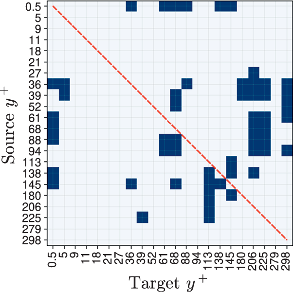
 are provided in Appendix A. For most interacting pairs, the null hypothesis is rejected, indicating that the corresponding TE values cannot be fully explained by preserved linear second-order structure alone and therefore suggesting a non-linear contribution to the interaction. Furthermore, the asymmetry of the matrix with respect to the main diagonal indicates that the evidence of a non-linear contribution to the pairwise interaction can itself be direction-dependent.
Matrix of rejection (light colour)/non-rejection (dark colour) outcomes for the Bi-IAAFT surrogate test (Pinto et al., Reference Pinto, Lazic, Antonacci, Pernice, Gu, Barà, Faes and Rocha2024) applied to TE between all interacting pairs of the simulation time series, using
$ k=10 $
 . Entries marked as rejected correspond to
$ p $
 -value less than
$ 0.05 $
 under the null hypothesis that the paired time series are exclusively linearly correlated. The dashed line shows the main diagonal of the matrix.

Figure 8. Long description
The matrix is a grid with the vertical y-axis labeled Source y plus and the horizontal x-axis labeled Target y plus. Both axes contain the same numerical values: 0.5, 5, 9, 11, 18, 21, 27, 36, 39, 52, 61, 68, 88, 94, 113, 138, 145, 180, 206, 225, 279, and 298. A red dashed diagonal line runs from the top-left corner (0.5, 0.5) to the bottom-right corner (298, 298).
Data points are represented by dark blue squares indicating rejected null hypotheses (p-value less than 0.05), while light grey squares indicate non-rejection. The distribution of dark blue squares is sparse and asymmetrical:
* Along the top row (Source 0.5), rejections occur at Target 36, 61, 68, 88, and 145.
* On the far left (Target 0.5), rejections are clustered at Source 36, 39, 61, 68, 88, 138, and 145.
* A significant cluster of rejections appears in the middle-right section, specifically between Source 36 to 94 and Target 206 to 225.
* Another vertical cluster of rejections is visible at Target 113, spanning Source 138 to 225.
* Isolated rejections are scattered throughout the lower-left and upper-right quadrants, with no rejections appearing for the highest Source or Target values (279 and 298).
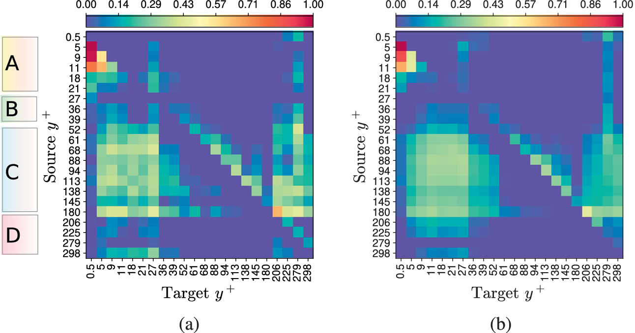
Despite the discrepancy between the TE values of the synthetic and simulation time series, we aim to investigate how much the synthetic data can preserve the correct dominant direction of information transfer between each time series pair. The net transfer entropy is defined in analogy with the flux in Massaro et al. (Reference Massaro, Rezaeiravesh and Schlatter2026). For this, we use normalised maximum TE which, for each interacting pair from the simulation data, is defined as,

A similar definition is used for the synthetic data, using the
$ {\max}_m\mathrm{TE} $
 values averaged over realisations. Here,
$ {\max}_{\mathrm{pair}} $
 denotes the maximum of the numerator in Equation (12) over all interacting pairs considered. Hence, the normalisation is performed globally over the full set of interacting pairs, but separately for the simulation and VAR-synthetic datasets. The resulting measure is plotted in Figure 9. There is a strong agreement between the two plots regarding the positions of non-zero values, indicating that the VAR model can effectively preserve the direction of the net information transfer for most of the time series pairs. A cautious conclusion could be that linear mechanisms dominate the underlying information transfer in these interactions. In contrast to the direction, the intensity of information flows is not necessarily preserved (under-predicted by the synthetic data). Further, compared to the ground truth, the VAR model is unable to capture the variation in the magnitude of the net maximum TE, and returns more uniform values in the plot.
Normalised net maximum TE defined in Equation (12) evaluated using the (a) simulation and (b) synthetic data (only the mean values are shown).

Figure 9. Long description
Two heatmaps, (a) simulation and (b) synthetic data, compare transfer entropy values.
Common Structure:
* Vertical Y-axis: Source y plus, with values ranging from 0.5 at the top to 298 at the bottom.
* Horizontal X-axis: Target y plus, with values ranging from 0.5 on the left to 298 on the right.
* Color Scale: A horizontal bar above each plot ranging from 0.00 (dark purple) to 1.00 (bright red/pink), passing through teal, green, and yellow.
* Left Sidebar: Four vertical regions labeled A, B, C, and D corresponding to different y plus ranges.
Panel (a) Simulation Data:
* High intensity (red/yellow) is concentrated in the top-left corner (Source y plus 0.5 to 11, Target y plus 0.5 to 9).
* A distinct diagonal line of moderate intensity (green/yellow) runs from the center toward the bottom-right.
* A vertical band of teal/green appears around Target y plus 206 to 298.
* The data appears granular with sharp transitions between neighboring grid cells.
Panel (b) Synthetic Data:
* Shows a similar global structure to panel (a) but with significantly smoother, blurred transitions.
* The high-intensity region in the top-left is less sharp.
* The central diagonal and the vertical band on the right are broader and more diffused compared to the simulation data.
The insights from Figure 9 are consistent with established findings in the turbulence literature regarding the interactions and directional relationships between different regions of a boundary layer. This suggests that statistical causality, quantified here by bivariate transfer entropy measuring directed pairwise interactions between such regions, can show consistency with relevant physical interpretations. For clarity, we examine zones
$ A $
 –
$ D $
 , whose boundaries are determined by the respective ranges of the source
$ {y}^{+} $
 :
$ A $
 :
$ {y}^{+}\lesssim 21 $
 ,
$ B $
 :
$ 27\lesssim {y}^{+}\lesssim 39 $
 ,
$ C $
 :
$ 52\lesssim {y}^{+}\lesssim 180 $
 , and
$ D $
 :
$ 206\lesssim {y}^{+}\lesssim 298 $
 . The values of the net maximum TE in zone
$ A $
 imply that the information transfer from the wall is strong only up to the location of maximum turbulent kinetic energy production (
$ {y}^{+}\lesssim 12 $
 ); see also Massaro et al. (Reference Massaro, Rezaeiravesh and Schlatter2026). This agrees with the intrusive causality studies by Flores and Jiménez (Reference Flores and Jiménez2006), Mizuno and Jiménez (Reference Mizuno and Jiménez2013), where the turbulence away from the wall could sustain after removing the near-wall region from simulations. Zone
$ B $
 corresponds to the buffer layer, and does not show any significant systematic directed interaction. Zone
$ C $
 can be considered as the logarithmic layer acting as an information source. As this layer is the overlap between the inner and outer regions of the boundary layer, its interactions are expected to be significant with different regions in the boundary layer. This is confirmed here, as Zone
$ C $
 exhibits directed pairwise interaction towards the near-wall region (up to
$ {y}^{+}\approx 39 $
 ), the wake region (
$ 206\lesssim {y}^{+}\lesssim 298 $
 ), and also higher target
$ {y}^{+} $
 within
$ 52\lesssim {y}^{+}\lesssim 180 $
 (visible in the non-zero upper diagonal elements in the plot). The net information transfer from the logarithmic layer towards Zones
$ A $
 and
$ B $
 is consistent with the baseline of hybrid and wall-modelled large eddy simulations (Larsson et al., Reference Larsson, Kawai, Bodart and Bermejo-Moreno2016), where the information from the core flow is used to model/reconstruct unresolved effects near the wall. Interestingly, the high net TE from Zone
$ D $
 to the near-wall region (
$ {y}^{+}\lesssim 27 $
 ) could provide evidence of top-down interactions that likely reflect the near-wall footprints (amplitude modulation) of the large structures; see Marusic et al. (Reference Marusic, Mathis and Hutchins2010), Mathis et al. (Reference Mathis, Monty, Hutchins and Marusic2009). It is emphasised again that a more in-depth physical interpretation would require the computation of multivariate TE.
4. Conclusions
In this study, we evaluate both linear and information-theoretic pairwise interactions between streamwise-velocity time series in a turbulent channel flow. The analysis considered CFD simulation data together with an ensemble of 50 synthetic datasets generated by a VAR model trained on the simulation data. The evaluation of the interactions between an extensive set of 231 time series pairs provides a detailed picture of the variation in different statistical measures across the entire turbulent channel flow boundary layer. The VAR synthetic data can completely preserve both concurrent and time-delayed linear relationships measured by autocorrelation and cross-covariance functions. Such agreement is expected, since the VAR formulation explicitly incorporates linear dependencies over multiple time lags. Moreover, these observations confirm that the selected model order (
$ p=60 $
 ) is appropriate. It is noteworthy that the VAR model with order 30 was also examined, which did not show a significant impact on the results.
The VAR synthetic data retained the time-delayed mutual information with a reasonable fidelity, demonstrating partial preservation of non-linear dependencies, despite slight spurious over-predictions. Transfer entropy, however, showed systematic under-predictions for most pairs relative to the simulation data. Despite this, the normalised net maximum transfer entropy of the VAR synthetic data was found to match relatively well with those obtained from the simulation time series. This measure can be utilised for identifying the direction of the dominant information flow within each time series pair. Therefore, an important conclusion is that a VAR model, with sufficiently high order, can properly predict the direction of information transfer despite inaccurately predicting its intensity. This suggests that linear interactions with longer time scales are dominant in the information transfer. Overall, the results indicate that a VAR model can effectively function as a model for turbulence time series synthesis, although its limitations should be acknowledged.
Transfer entropy is commonly used as a statistical measure of causality. In this study, we observed that bivariate TE, despite its limitations, can yield patterns that are consistent with relevant physical causality reported in the turbulence literature, particularly across different regions of boundary layers (Jiménez, Reference Jiménez2013; Lozano-Durán et al., Reference Lozano-Durán, Bae and Encinar2019; Martínez-Sánchez et al., Reference Martínez-Sánchez, Arranz and Lozano-Durán2024; Massaro et al., Reference Massaro, Rezaeiravesh and Schlatter2026; Zhang et al., Reference Zhang, Zhu, Wang and Hu2025). Specifically, this study showed the importance of employing optimal delays for accurate estimation of TE. For optimisation, we used the auto-mutual information function, which showed a shorter integral time scale than the autocorrelation function. According to Appendix B, using the default embedding delay can significantly affect the computed values of transfer entropy, particularly for VAR synthetic data. In addition, the choice of estimator for the non-linear interaction measures was found to be important. The results presented in the main body of the paper were obtained using the KSG estimators (Kraskov et al., Reference Kraskov, Stögbauer and Grassberger2004; Frenzel and Pompe, Reference Frenzel and Pompe2007) with
$ k=10 $
 . As shown in Appendix A, varying the value of
$ k $
 has some influence on the results, see also Stoļarovs et al., Reference Stoļarovs, Toosi, Yang, Massaro, Garcia, Yao, Mihajlović, Hussain, Rezaeiravesh and Schlatter2026, although this effect is considerably smaller than the impact of switching to a KDE-based estimator.
Given the non-intrusive nature and significance of the analyses performed in this study, we recommend applying the same methodology to synthetic or forecasted turbulence time series generated by other models. This is crucial for assessing the degree to which such data preserve the underlying physical interactions and statistical dependencies found in simulations or experiments.
The present study can be extended in several directions. To better capture the rare and extreme turbulent events, moving-average terms can be incorporated into the VAR model. The velocity time series used here were spatially averaged over the homogeneous direction of the channel flow, which might influence the performance of the VAR model. Repeating the analyses particularly at higher Reynolds numbers where scale separation is more pronounced should also be considered. Finally, this study focused exclusively on pairwise transfer entropy. To enhance physical interpretability and identify the actual drivers within the turbulent causal network, future works will incorporate multivariate transfer entropy.
Data availability statement
The source code and turbulent channel flow time series data used to compute the interactions in this study are available at: https://github.com/simFlowDataLab/pairwiseValidation_turbulenceTS (Rezaeiravesh et al., Reference Rezaeiravesh, Massaro and Schlatter2026).
Acknowledgements
This work used the ARCHER2 UK National Supercomputing Service (https://www.archer2.ac.uk). The authors would like to thank the UK EPSRC for providing computational time for the computations on ARCHER2 via the UK Turbulence Consortium (EP/D44073/1 and EP/G06958/1).
Author contribution
Conceptualisation: S.R., D.M., P.S.; Methodology: S.R., D.M.; Software: S.R.; Data curation: S.R.; Visualisation: S.R.; Formal analysis: S.R., D.M.; Writing original draft: S.R; Writing—review & editing: D.M., P.S. All authors approved the final submitted draft.
Funding statement
D.M. acknowledges the financial support provided by the Knut and Alice Wallenberg Foundation.
Competing interests
The authors declare none.
Ethical standard
The research meets all ethical guidelines, including adherence to the legal requirements of the study country.
Appendices
Appendix A: Impact of the estimator on the information-theoretic measures
The mutual information and transfer entropy in this study are estimated using the KSG estimator from Equations (8) and (10), respectively. These estimators can be sensitive to the value of
$ k $
 . The results obtained from default
$ k=10 $
 in Figures 4, 7, and 9, can be compared to the case of using
$ k=5 $
 and
$ k=30 $
 in Figure A1 (the first and second rows, respectively). The general pattern in the maximum MI and TE is not affected, and particularly the main features in the net maximum TE are largely preserved. However, the upper bound for the maximum TE is significantly reduced with increasing
$ k $
 . In such cases, the estimator will consider larger neighbourhoods around each sample over which the density is assumed to be constant. Therefore, for high values of
$ k $
 , there should be a smoothing effect resulting in larger bias and lower variance. Although the selection of
$ k $
 is not, in general, trivial and could be optimised (Witter and Houghton, Reference Witter and Houghton2024), in this study we choose
$ k=10 $
 . In contrast, the use of the KDE estimator, the bottom row in Figure A1, can lead to over-smoothing and large bias in the estimations. In particular, the maximum TE and its net value are different from those by the KSG estimator even with
$ k=30 $
 .
Mean of the (left column) maximum time-delayed MI, (middle column) maximum TE, and (right column) normalised net maximum TE estimated from VAR synthetic data using (top row) the KSG estimator with
$ k=5 $
 , (middle row) the KSG estimator with
$ k=30 $
 , and (bottom row) the KDE estimator.

Figure A1. Long description
The grid consists of nine heat maps organized into three rows and three columns.
Vertical and Horizontal Axes: All panels share the same axes. The vertical axis is labeled Source y plus and the horizontal axis is labeled Target y plus. Both axes feature discrete numerical values ranging from 0.5 to 298.
Columnar Organization:
- Left Column: Displays maximum time-delayed M I. The heat maps show a strong diagonal trend from top-left to bottom-right with values peaking near 3.34.
- Middle Column: Displays maximum T E. These panels show a broader distribution of values across the grid compared to M I, with a prominent diagonal and higher values in the upper-right quadrant.
- Right Column: Displays normalized net maximum T E. These panels are characterized by a sparse diagonal of high values (near 1.00) against a predominantly dark blue background.
Row-wise Estimator Comparison:
- Top Row: K S G estimator with k = 5. Shows relatively smooth gradients in the M I and T E plots.
- Middle Row: K S G estimator with k = 30. Shows similar patterns to the top row but with slightly different intensity scales, particularly in the T E plot where the maximum value is 0.48 compared to 1.48 in the top row.
- Bottom Row: K D E estimator. The M I plot shows more distinct, blocky regions of lower values in the bottom-left. The T E plot in this row has a much lower maximum value of 0.69 and a more uniform light-yellow background in the upper-right region.
Color Scales: Each panel has an individual horizontal color bar at the top, transitioning from dark blue (low) through green and yellow to dark red (high).
The choice of
$ k $
 also affects surrogate-based hypothesis testing. For the source-row-shuffling surrogate (Pinto et al., Reference Pinto, Lazic, Antonacci, Pernice, Gu, Barà, Faes and Rocha2024), the associated null hypothesis is rejected for all three values
$ k=5,10 $
 , and
$ 30 $
 , indicating that the estimated TE values remain statistically significant under this null. For the Bi-IAAFT surrogate (Pinto et al., Reference Pinto, Lazic, Antonacci, Pernice, Gu, Barà, Faes and Rocha2024), however, the effect of
$ k $
 is more pronounced. Comparing Figure 8 with Figure A2 shows that increasing
$ k $
 reduces the number of pairs for which the Bi-IAAFT null hypothesis is rejected. This suggests that larger values of
$ k $
 make departures from the linear-surrogate null harder to detect, which is consistent with the stronger smoothing effect induced by larger neighbourhoods in the KSG estimator.
Matrix of rejection (light colour)/non-rejection (dark colour) outcomes for the Bi-IAAFT surrogate test (Pinto et al., Reference Pinto, Lazic, Antonacci, Pernice, Gu, Barà, Faes and Rocha2024) applied to TE between all interacting pairs of the simulation time series, using (a)
$ k=5 $
 and (b)
$ k=30 $
 . Entries marked as rejected correspond to p-value less than
$ 0.05 $
 under the null hypothesis that the paired time series are exclusively linearly correlated. The dashed line shows the main diagonal of the matrix.

Figure A2. Long description
Two side-by-side square matrices, labeled a and b, display the results of a statistical test. Both matrices share identical axes: the vertical axis is labeled Source y plus and the horizontal axis is labeled Target y plus. The axis values range from 0.5 at the top-left to 298 at the bottom-right. A red dashed diagonal line runs from the top-left corner to the bottom-right corner of both plots.
Panel a, representing k equals 5, shows a sparse distribution of dark blue squares against a light gray background. The dark blue squares, representing rejected null hypotheses, are primarily clustered in the middle-left and bottom-center regions of the matrix, with a notable horizontal band near the top-right edge.
Panel b, representing k equals 30, shows a significantly higher density of dark blue squares compared to panel a. The blue squares are distributed more broadly across the entire matrix, though there is a higher concentration in the left half and the bottom-right quadrant. In both panels, the dark blue squares are generally located away from the red dashed main diagonal.
Additional sensitivity analyses with representative interacting pairs in Section 3, using different sample lengths
$ n $
 and several values of
$ k $
 , did not reveal a single uniformly optimal choice of
$ k $
 . Nevertheless, they showed that the main qualitative conclusions, particularly the sign of the net maximum TE for the representative pairs considered, are robust for
$ 10\le k\le 40 $
 and n = 10,437. This further supports the use of
$ k=10 $
 as a pragmatic intermediate choice. Furthermore, because the same value of
$ k $
 is used consistently for both the simulation and the VAR-synthetic data, any residual estimator bias is of secondary importance for the comparative aim of the present study.
Appendix B: Impact of the embedding delay value on TE estimates
In Section 3, for computing the TE, the embedding delay
$ \tau $
 in Equation (7) was optimised for all the interacting time series. This is a crucial step, noting that the default value of
$ \tau =1 $
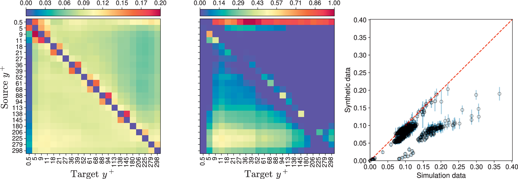
 in Figure B1 leads to largely under-predicted TEs compared to Figure 7. Moreover, the pattern of the net maximum TE is largely affected, and for many pairs, the maximum TE values of the synthetic data are found to be significantly underpredicted compared to those of the simulation data. These clearly show that
$ \tau =1 $
 is too small to provide any new information about the past of a source time series. This redundancy is, however, intuitive, reminding the slow decay in both ACF and AMIF in Figures 3 and 5a, respectively.
Mean of (a) maximum TE and (b) net maximum TE obtained from the VAR synthetic data. (c) Scatter plot of the maximum TE obtained from the VAR synthetic data and simulation data. All TE are estimated using embedding delay
$ \tau =1 $
 in Equation (7). The KSG estimator with
$ k=10 $
 is used.

Figure B1. Long description
A three-panel figure analyzing Transfer Entropy (T E).
Panel a, a heatmap titled Mean of maximum T E. The vertical y-axis is labeled Source y plus and the horizontal x-axis is labeled Target y plus. Both axes have discrete values ranging from 0.5 to 298. A color bar at the top ranges from 0.00 (blue) to 0.20 (pink). The heatmap shows a strong diagonal trend of high T E values (red and orange squares) where source and target values are similar, surrounded by a gradient of lower values (yellow and green).
Panel b, a heatmap titled Mean of net maximum T E. It uses the same axes as panel a. The color bar at the top ranges from 0.00 (blue) to 1.00 (pink). This plot shows a more sparse distribution with a distinct diagonal of high-intensity points (yellow and light green) and a concentrated region of higher values in the bottom-left corner, while the rest of the field is mostly dark blue (near zero).
Panel c, a scatter plot comparing Synthetic data on the y-axis to Simulation data on the x-axis, both ranging from 0.00 to 0.40. A red dashed diagonal line represents a one-to-one correlation. Data points are represented by open circles with vertical error bars. The points are clustered into two main groups: one group follows the red dashed line closely up to 0.15, and a second group forms a lower-sloped linear cluster below the diagonal line, extending toward the bottom-right.













 Open access


Comments
No Comments have been published for this article.