1. Introduction
The study of risk-sensitive Markov decision processes in discrete time started in the 1970s [Reference Howard and Matheson16], and there have since been a lot of developments; see, e.g., [Reference Bäuerle and Rieder2, Reference Cavazos-Cadena and Hernández-Hernández3, Reference Cavazos-Cadena and Montes-de-Oca4, Reference Di Masi and Stettner5, Reference JaŚkiewicz19, Reference Karel20]. In comparison, there has been limited work on risk-sensitive continuous-time Markov decision processes (CTMDPs). For background on risk-sensitive CTMDPs, see [Reference Ghosh and Saha7, Reference Guo and Liao11, Reference Kumar and Pal22] for the risk-sensitive (infinite-horizon) discounted criterion, [Reference Ghosh and Saha7, Reference Kumar and Pal22, Reference Kumar and Pal23, Reference Wei and Chen25, Reference Wei and Chen26, Reference Wei and Chen27] for the risk-sensitive (long-run) average criterion, [Reference Ghosh and Saha7, Reference Guo, Liu and Zhang9, Reference Guo and Zhang14, Reference Huang, Lian and Guo17, Reference Huang, Lian and Guo18, Reference Kumar and Pal23, Reference Wei24] for the risk-sensitive finite-horizon criterion, and [Reference Guo and Zhang8, Reference Zhang28] for the risk-sensitive total cost criterion. In this paper we will further consider the risk-sensitive average criterion for CTMDPs studied in [Reference Ghosh and Saha7, Reference Kumar and Pal22, Reference Kumar and Pal23, Reference Wei and Chen25, Reference Wei and Chen26, Reference Wei and Chen27]. More precisely, [Reference Ghosh and Saha7] proved the existence of an optimal policy under the geometric ergodicity assumption and Doeblin-type conditions for the small cost function and bounded transition rates, and provided a policy improvement algorithm for the case of finite states and actions, but they did not establish a characterization of the optimality equation. Using the multiplicative dynamic programming principle, [Reference Kumar and Pal22] proved the existence and a characterization of an optimal policy under the positive recurrent assumption for a near-monotone cost function and bounded transition rates, and [Reference Kumar and Pal23] under the geometric ergodicity conditions of the state dynamics for small running cost and bounded transition rates. Wei and Chen [Reference Wei and Chen25, Reference Wei and Chen26] considered the case of finite states under the ergodicity condition. The arguments for the existence of an average optimal deterministic stationary policy in [Reference Ghosh and Saha7, Reference Kumar and Pal22, Reference Kumar and Pal23, Reference Wei and Chen25, Reference Wei and Chen26] are based on the ergodicity conditions and assumptions of bounded transition rates. For a general case of unbounded cost and transition rates, [Reference Wei and Chen27] proved the existence of an optimal policy under irreducibility and Doeblin’s conditions, using the risk-sensitive average optimality inequality. Moreover, only stationary policies were considered in [Reference Wei and Chen25], whereas the general class of Markov policies was taken into account in [Reference Ghosh and Saha7, Reference Kumar and Pal22, Reference Kumar and Pal23, Reference Wei and Chen25, Reference Wei and Chen26, Reference Wei and Chen27].
In the present work we will further study the general case that the transition and cost rates are allowed to be unbounded. We not only establish the existence and uniqueness of a solution to the risk-sensitive average optimality equation (RS-AOE) and prove the existence of an optimal stationary policy via the RS-AOE, but also provide an approximation algorithm for computing average optimal policies. Our arguments are inspired by those of [Reference Kumar and Pal23] in constructing a solution to the RS-AOE, which is more specific than the risk-sensitive average optimality inequality in [Reference Wei and Chen27]. Apart from allowing unbounded transition and cost rates, we consider a more general class of randomized history-dependent policies, and do not require the condition that the controlled process is irreducible under each deterministic stationary policy, where the irreducibility condition was also assumed in [Reference Ghosh and Saha7, Reference Kumar and Pal22, Reference Kumar and Pal23, Reference Wei and Chen25, Reference Wei and Chen26, Reference Wei and Chen27]. Some of our conditions are extensions of those in [Reference Ghosh and Saha7, Reference Kumar and Pal22, Reference Kumar and Pal23] and different from those in [Reference Wei and Chen27]; see Remarks 3.1, 3.3, 7.2, and 7.3 for more details.
First, under the milder conditions from [Reference Guo, Liu and Zhang9, Reference Guo and Piunovskiy12, Reference Guo and Zhang14], as in the arguments of [Reference Ghosh and Saha7, Reference Kumar and Pal23] we derive the multiplicative dynamic programming principle and obtain some interesting results, such as the existence and uniqueness of a solution to the optimality equation and properties of the value function for risk-sensitive finite-horizon CTMDPs with unbounded transition and cost rates (Theorem 3.1 and Lemma 3.2). Second, using the multiplicative dynamic programming principle and properties developed here for risk-sensitive finite-horizon CTMDPs, by the method in [Reference Ghosh and Saha7, Reference Kumar and Pal23] we obtain the existence of a solution to the RS-AOE and its characterization for risk-sensitive average CTMDPs (Theorems 4.1 and 6.2). Third, to prove the existence of a risk-sensitive average optimal policy via the RS-AOE, we provide some new and verifiable sufficient conditions under which we prove that the solution to the RS-AOE is bounded away from zero (Proposition 5.1), and under which we establish the existence of a risk-sensitive average optimal stationary policy over the class of all randomized history-dependent policies (Theorem 5.1). Fourth, after showing the solvability of the multiplicative Poisson equation, we construct a sequence of models of finite-state CTMDPs for which the corresponding optimal stationary policies can be obtained by the policy iteration algorithm in a finite number of iterations (Theorem 6.1), and further prove that an average optimal policy for the case of infinitely countable states can be approximated by those of the finite-state models (Theorem 6.2). Finally, in order to illustrate our conditions and the main results, we present an example on a controlled population with unbounded transition rates and cost functions [Reference Anderson1], in which all of our conditions are satisfied, while some of the conditions in [Reference Ghosh and Saha7, Reference Kumar and Pal22, Reference Kumar and Pal23, Reference Wei and Chen25, Reference Wei and Chen26, Reference Wei and Chen27] fail to hold; see Remarks 7.2 and 7.3. Also, we conduct a numerical experiment to show the effectiveness of the finite-approximation policy iteration algorithm.
The rest of the paper is organized as follows. We describe the optimization problem in Section 2, and derive the multiplicative dynamic programming principle and some new facts for risk-sensitive finite-horizon CTMDPs in Section 3, where some comments on our conditions are given by Remarks 3.1, 3.3, and 3.4 and Example 3.1. We establish the existence of an optimal policy in Section 5, after establishing the RS-AOE in Section 4. We provide a finite-approximation algorithm for computing optimal policies and prove its convergence in Section 6, and illustrate our main results with an example in Section 7. Finally, we provide an appendix for the proofs of some preliminaries in Section 8.
2. The risk-sensitive average optimality problem
The model of CTMDPs is a four-tuple,  $\mathbb{M}\,:\!=\{S, A(i), c(i,a), q(\,j \mid i,a)\}$, consisting of the following elements:
• a denumerable set S, called the state space, whose elements are referred to as states of a system (for simplicity, without loss of generalization, let
 $S\,:\!=\{0,1, \ldots,i,\ldots\}$);
• the action sets A(i), each of which denotes the set of actions available to a controller when the system is in state
$i\in S$, and is assumed to be a compact subset of a Borel space A;• the running cost rate function c(i, a) that is assumed to be real valued, Borel measurable, and bounded from below on K, where
$K\,:\!=\{(i,a) \mid i\in S,a\in A(i)\}$;• the transition rates
$q(\,j \mid i,a)$, a Borel-measurable signed kernel on S given K, taking nonnegative values for all $j,i\in S$ with $j\not=i$, being conservative in the sense of $q(S \mid i,a)\equiv 0$, and stable in that of
(1)where
\begin{eqnarray} q^{*}(i)\,:\!=\,\sup_{a\in A(i)}q(i,a)<\infty \qquad \text{for all } i\in S, \end{eqnarray}
$q(i,a)\,:\!=\,-q(i \mid i,a)\geq0$ for all $(i,a)\in K$.







To formalize this, below we show the construction of CTMDPs under possibly randomized history-dependent policies. To do so, we introduce some notation. Let  $S_\Delta\,:\!=\,S\cup\{\Delta\}$ (with some
 $\Delta\not\in S$),
 $\Omega^{0}\,:\!=\,(S\times(0,\infty))^{\infty}$,
 \begin{multline*} \Omega\,:\!=\,\Omega^{0}\cup\{(i_{0},\theta_{1},i_{1},\ldots,\theta_{k},i_{k}, \infty,\Delta,\infty, \ldots) \mid i_0, i_{l}\in S, \theta_{l}\in(0,\infty) \\ \text{ for each } 1\leq l\leq k, k\geq1\},\end{multline*}
and let  $\mathcal{F}$ be the Borel
 $\sigma$-algebra on
 $\Omega$. Then we obtain the measurable space
 $(\Omega,\mathcal{F})$. For each
 $k\geq 0$ and
 $\omega\,:\!=\,(i_{0},\theta_{1},i_{1},\ldots,\theta_{k},i_{k},\ldots) \in \Omega$, let
 $h_{k}(\omega)\,:\!=\,(i_{0},\theta_{1},i_{1},\ldots,\theta_{k},i_{k})$ denote the k-component internal history, and define
 $T_{0}(\omega)\,:\!=\,0$,
 $T_{k+1}(\omega)\,:\!=\,\theta_{1}+\theta_{2}+\cdots+\theta_{k+1}$,
 $X_k(\omega)\,:\!=\,i_k$. In what follows, the argument
 $\omega$ is always omitted. Let
 $T_{\infty}\,:\!=\,\lim_{k\rightarrow\infty}T_{k}$, and define the continuous-time process
 $\{x_t\}$ by
 \begin{eqnarray} x_t\,:\!=\,\sum_{k\geq0}\mathbf{1}_{\{T_{k}\leq t<T_{k+1}\}}X_{k}+\Delta \mathbf{1}_{\{t\geq T_\infty\}} \qquad \textrm{for } \ t\geq 0.\end{eqnarray}
Here and below,  $\mathbf{1}_{E}$ stands for the indicator function on any set E, and we use the notation that
 $0+z=z$ and
 $0z=0$ for all
 $z\in S_\Delta$.
From (2), we see that  $T_{k}$ (
 $k\geq 1$) denotes the kth jump moment of
 $\{x_t\}$,
 $X_{k-1}$ is the state of the process on
 $[T_{k-1},T_k)$, and
 $\Theta_{k}\,:\!=\,T_{k}-T_{k-1}$ plays the role of sojourn time at state
 $X_{k-1}$. We do not intend to consider the controlled process after moment
 $T_\infty$, and thus view it to be absorbed in the state
 $\Delta$. Hence, we write
 $q(\cdot \mid \Delta,a_\Delta):\equiv 0$,
 $c(\Delta,a_\Delta):\equiv0$,
 $A(\Delta)\,:\!=\{a_\Delta\}$,
 $A_\Delta\,:\!=\,A\cup\{a_\Delta\}$, where
 $a_\Delta$ is an isolated point.
To state the optimality problem, we need to introduce the concept of a policy [Reference Guo, Liu and Zhang9, Reference Guo, Huang and Huang15, Reference Kitaev and Rykov21].
Definition 2.1. A randomized history-dependent policy  $\pi$ is determined by a sequence
 $\{\pi^k,k\geq 0\}$ such that
 \begin{align*}\pi(\textrm{d} a \mid \omega,t) & = \mathbf{1}_{\{0\}}(t)\pi_{0}(\textrm{d} a \mid i_{0},0)+\sum_{k\geq 0}\mathbf{1}_{\{T_{k}<t\leq T_{k+1} \}}\pi^{k}(\textrm{d} a \mid i_{0},\theta_{1},i_{1},\ldots,\theta_{k},i_{k},t-T_{k}) \\& \quad + \mathbf{1}_{\{t\geq T_{\infty}\}}\delta_{a_\Delta}(\textrm{d} a), \end{align*}
where  $\pi_{0}(\textrm{d} a \mid i_0,0)$ is a stochastic kernel on A given S such that
 $\pi_{0}(A(i_0) \mid i_0,0)=1$,
 $\pi^{k}$
 $(k\geq 0)$ are stochastic kernels on A given
 $(S\times(0,\infty))^{k+1}$ such that
 $\pi^{k}(A(i_k) \mid i_{0},\theta_{1},i_{1},\ldots,\theta_{k},i_{k},t-T_{k})=1$, and
 $\delta_{a_\Delta}(\textrm{d} a)$ denotes the Dirac measure at the point
 $a_\Delta$.
A policy  $\pi$ is called randomized Markovian if each
 $\pi^k$ has the form
 $\pi^k(\textrm{d} a \mid i_k,t)$ (independent of the histories
 $(i_{0},\theta_{1},i_{1},\ldots,\theta_{k})$), and it will be denoted by
 $\pi_t(\textrm{d} a \mid \cdot)$. A randomized Markov policy
 $\pi_t(\textrm{d} a \mid \cdot)$ is called deterministic Markovian whenever there exists an A-valued Borel-measurable function
 $f_t(i)$ on
 $[0,\infty)\times S$ such that
 $\pi_{t}(\textrm{d} a \mid i)$ is a Dirac measure concentrated at
 $f_t(i)$ for each
 $(t,i)\in [0,\infty)\times S$. Such a Markov policy will be denoted by
 $f_t$ for simplicity. A Markov policy
 $f_t$ is called a (deterministic) stationary one if
 $f_t$ is independent of time t. Such a stationary policy will be denoted by f for simplicity.
We denote by  $\Pi$ the set of all randomized history-dependent policies, by
 $\Pi_\textrm{m}^\textrm{r}$ the set of all randomized Markov policies, by
 $\Pi_\textrm{m}^\textrm{d}$ the set of all (deterministic) Markov policies, and by F the set of all stationary policies. Obviously,
 $\Pi\supset\Pi_\textrm{m}^\textrm{r}\supset\Pi_\textrm{m}^\textrm{d}\supset F$.
For any initial distribution  $\gamma$ on S and policy
 $\pi\in\Pi$, we introduce the unique probability measure
 $\mathbb{P}_{\gamma}^{\pi}$ on
 $(\Omega,\mathcal{F})$ as in [Reference Guo and Piunovskiy12, Reference Guo and Song13, Reference Zhang28]. Let
 $\mathbb{E}_\gamma^{\pi}$ be its corresponding expectation operator. In particular,
 $\mathbb{E}_\gamma^\pi$ and
 $\mathbb{P}_\gamma^\pi$ will be respectively written as
 $\mathbb{E}_i^\pi$ and
 $\mathbb{P}_i^\pi$ when
 $\gamma$ is the Dirac measure located at a state i in S.
As in [Reference Ghosh and Saha7, Reference Kumar and Pal22, Reference Kumar and Pal23, Reference Wei and Chen25], the risk-sensitive average criterion of CTMDPs is defined by
 \begin{eqnarray*} J(i,\pi)\,:\!=\,\limsup_{T\to\infty}\frac{1}{T}\ln\mathbb{E}_{i}^{\pi}\left[\exp\left\{\int_{0}^{T}\int_{A}c(x_t,a)\pi(\textrm{d} a \mid \omega,t) \, \textrm{d} t\right\}\right] \end{eqnarray*}
for each  $i\in S$ and
 $\pi\in \Pi$.
Definition 2.2. A policy  $\pi^{*}\in\Pi$ is said to be risk-sensitive (R-S) average optimal if
 $J(i,\pi^*)=\inf_{\pi\in \Pi}J(i,\pi)$ for all
 $i\in S$.
This paper will give new conditions for the existence and computation of R-S average optimal stationary policies.
Since c(i, a) is bounded below (i.e.  $c(i,a)\geq L$ for all
 $(i,a)\in K$ and some constant L), we have
 $c(i,a)+|L|\geq 0$ on K, and
 \begin{equation*}\limsup_{T\to\infty}\frac{1}{T}\ln\mathbb{E}_{i}^{\pi}\left[\exp\left\{\int_{0}^{T}\int_{A}[c(x_t,a)+|L|]\pi(\textrm{d} a \mid \omega,t) \, \textrm{d} t\right\}\right]=J(i,\pi)+|L|.\end{equation*}
Thus, adding a constant to all the costs c(i, a) will affect all policies identically under the R-S average criterion. Therefore, without loss of generality, we will further assume that c(i, a) is nonnegative on K.
3. Preliminaries
To prove the existence of risk-sensitive average optimal policies, we need to develop some preliminary facts concerning risk-sensitive finite-horizon CTMDPs, some of which are from [Reference Guo, Liu and Zhang9] and some of which are new.
3.1. Non-explosion and finiteness
Since the transition and cost rates may be unbounded, we need the following conditions from [Reference Guo, Liu and Zhang9, Reference Guo and Piunovskiy12, Reference Guo, Huang and Huang15, Reference Kumar and Pal23] to guarantee the non-explosion of  $\{x_t,t\geq 0\}$ and the finiteness of
 $J(i,\pi)$.
Assumption 3.1. There exist real-valued functions  $V_0\geq 1$ and
 $\delta \geq 0$ on S, positive constants
 $b_0$ and
 $M_0$, and a state
 $i_0\in S$ such that:
(i)
$\sum_{j\in S}V_0(\,j)q(\,j \mid i,a)\leq -\delta(i)V_0(i)+b_0\mathbf{1}_{\{i_0\}}(i)$ for all $(i,a)\in K$;-
(ii)
$q^*(i)\leq M_0V_0(i)$ for all $i\in S$, where $q^*(i)$ is as in (1); -
(iii)
$\delta_*\,:\!=\,\inf_{i\neq i_0}\delta(i)>0$ and $0\leq c(i,a)\leq \delta(i)\leq \sqrt{\ln V_0(i)}$ for all $(i,a)\in K$.



(a) Although the indicator function
$\mathbf{1}_{\{i_0\}}$ in Assumption 3.1(i) is a modification of the indicator function $\mathbf{1}_{C}$ in [Reference Kumar and Pal23] with a finite subset C of S, such a modification is required; see Remark 3.4 for more details. Assumption 3.1(i) is an extension of Assumption (A2) in [Reference Kumar and Pal23], Assumption (A5) in [Reference Ghosh and Saha7], Assumption 3.1(i) in [Reference Wei and Chen27], and Assumption 7.1 in [Reference Guo and Hernández-Lerma10], from a constant $\delta$ in [Reference Ghosh and Saha7, Reference Guo and Hernández-Lerma10, Reference Kumar and Pal23, Reference Wei and Chen27] to a function $\delta(i)$ on S here. Thus, it is satisfied for the examples in [Reference Ghosh and Saha7, Reference Guo and Hernández-Lerma10] and will be verified with other examples below.-
(b) Assumption 3.1(iii) is new and ensures the finiteness of
where
\begin{equation*}\mathbb{E}_{i}^{\pi}\left[\exp\left\{\int_0^{\tau_{i_0}}\int_Ac(x_v,a)\pi(\textrm{d} a \mid \omega,v) \, \textrm{d} v\right\}\right],\end{equation*}
$\tau_{i_0}\,:\!=\,\min\{t\geq 0 \mid x_t=i_0\}$ denotes the first passage time to $i_0$. Since the function c(i, a) here is allowed to be unbounded, Assumption 3.1(iii) is an extension of the so-called smallness condition (i.e. $\sup_{(i,a)\in K} |c(i,a)|<\delta_*$) in [Reference Ghosh and Saha7, Reference Kumar and Pal23] and different from the near-monotone condition in [Reference Kumar and Pal22]; see Example 7.1 and Remark 7.3 for details.
-
(c) Although Assumption 3.1(i) is slightly stronger than Assumption 3.1(i) in [Reference Wei and Chen27], Assumptions 3.3(ii) and 3.4(ii) in [Reference Wei and Chen27] are not required here.


To characterize risk-sensitive CTMDPs over the class of all history-dependent policies, we need an extension of the Feymanm–Kac formula in [Reference Guo, Liu and Zhang9] from the Markovian case to a more general case, which is based on the following conditions.
Assumption 3.2. There exist a real-valued function  $V_1 \geq 1$ on S and positive constants
 $\rho_1$,
 $b_1$, and
 $M_1$ such that:
(i)
$\sum_{j\in S}V_1^2(\,j)q(\,j \mid i,a)\leq \rho_1V_1^2(i)+b_1$ for all $(i,a)\in K$;-
(ii)
$V_0^2(i)\leq M_1V_1(i)$ for all $i\in S$, where $V_0$ comes from Assumption 3.1.


It can be proved that Assumption 3.2 is not required when the transition rates are bounded (i.e.  $\sup_{j\in S, (i,a)\in K} |q(\,j \mid i,a)|<\infty$).
(i) For any fixed
$i,j\in S$, $q(\,j \mid i,a)$ and c(i, a) are continuous in $a\in A(i)$;-
(ii) For any given
$i \in S$, the convergence of $\sum_{j\in S}V_0(\,j)q(\,j \mid i,a)$ holds uniformly in $a\in A(i)$.


Remark 3.2. Assumption 3.3(ii) is an extension of (A3) in [Reference Ghosh and Saha7]. Moreover, under Assumption 3.3(i), Assumption 3.3(ii) is fulfilled automatically when  $\sum_{j\in S(i)}q(\,j \mid i,a)=0$ for
 $a\in A(i)$, where S(i) is a finite subset of S and can depend on
 $i\in S$. Assumption 3.3 implies that
 $\sum_{j\in S}V_0(\,j)q(\,j \mid i,a)$ is continuous in
 $a\in A(i)$, and so is slightly stronger than the continuity–compactness conditions [Reference Ghosh and Saha7, Reference Kumar and Pal22, Reference Kumar and Pal23]. In fact, it is required not only for the facts in [Reference Guo, Liu and Zhang9] but also for the existence of
 $\varphi'(t,i)$ at all
 $t\geq 0$ in Theorem 3.1 (instead of at almost everywhere
 $t\geq 0$ in [Reference Kumar and Pal23]); see Remark A.1 for more details.
Lemma 3.1. If Assumptions 3.1 and 3.2 are satisfied, then the following assertions hold:
(a) For
$i\in S$ and $\pi\in \Pi$,
\begin{equation*}\mathbb{E}_{i}^{\pi}\left[\exp\left\{\int_0^{\tau_{i_0}}\int_Ac(x_v,a)\pi(\textrm{d} a \mid \omega,v) \, \textrm{d} v\right\}\right]\leq \mathbb{E}_{i}^{\pi}\left[\exp\left\{\int_0^{\tau_{i_0}}\delta(x_v) \, \textrm{d} v\right\}\right]\leq V_0(i).\end{equation*}
-
(b)
$\mathbb{E}_{i}^{\pi}[\tau_{i_0}]\leq \frac{V_0(i)}{\delta_*}$ and $\mathbb{P}_{i}^{\pi}(\tau_{i_0}<\infty)=1$, for all $i\in S$ and $\pi\in\Pi$.


Proof. See Appendix A.
Remark 3.3. In this paper,  $i_0$ in Lemma 3.1 comes directly from Assumption 3.1(i). However, in [Reference Kumar and Pal23], the corresponding reference state
 $i_0$ is determined by the condition
 $V(i_0)\geq 1+\frac{b}{\delta}$, where the function V and constants
 $\delta$ as well as b are from [Reference Kumar and Pal23, Assumption A2], corresponding to the
 $V_0$ and
 $\frac{\delta(i)}{2}$ as well as
 $b_0$ in Assumption 3.1 here. Example 3.1 shows that the condition
 $V(i_0)\geq 1+\frac{b}{\delta}$ actually cannot be used to get a reference state.
Example 3.1. Let  $S\,:\!=\{0,1,2\}$, all A(i) be singleton sets; then there is a unique stationary policy, say f. Moreover, let
 $q(0 \mid 0,f(0)) = -1$,
 $q(1 \mid 0,f(0)) = 1$,
 $q(2 \mid 0,f(0)) = 0$;
 $q(0 \mid 1,f(1)) = 8$,
 $q(1 \mid 1,f(1)) = -9$,
 $q(2 \mid 1,f(1)) = 1$;
 $q(0 \mid 2,f(2)) = 0$,
 $q(1 \mid 2,f(2)) = 8$,
 $q(2 \mid 2, f(2)) = -8$.
Obviously, Assumption A2 in [Reference Kumar and Pal23] is satisfied for  $V(i)\,:\!=\,3+i$ for
 $i\in S$,
 $C\,:\!=\{0,1\}$ (or
 $\{0\}$),
 $\delta\,:\!=\,\frac{1}{2}$,
 $b\,:\!=\,4$, which implies that
 $1+\frac{b}{\delta}=9>V(i)$ for all
 $i\in S$. Thus, if we follow the statement in [Reference Kumar and Pal23], this example does not have any reference state.
However, since Assumptions 3.1 and 3.2 are also satisfied for  $V_0(i)=V_1(i)\,:\!=\,3+i$ for
 $i\in S$ and
 $i_0=0$, the state 0 is actually a reference state for this paper.
3.2. Finite-horizon optimality
In order to deal with risk-sensitive average optimality, we need some notation and facts on risk-sensitive finite-horizon optimality.
For any  $\pi\in \Pi$,
 $t\geq 0$,
 $i\in S$, the t-horizon risk-sensitive criterion
 \begin{eqnarray*} \varphi(t,i,\pi)\,:\!=\,\mathbb{E}_i^{\pi}\left[\exp\left\{\int_0^t\int_{A}c(x_s,a)\pi(\textrm{d} a \mid \omega,s) \, \textrm{d} s\right\}\right] \end{eqnarray*}
is well defined. Then, let  $\varphi(t,i)\,:\!=\, \inf_{\pi\in \Pi}\varphi(t,i,\pi)$ for
 $i\in S$, which is called the value function of the t-horizon risk-sensitive criterion. Since c is nonnegative,
 $\varphi (t,i)$ is increasing in
 $t\geq 0$,
 $\varphi (0,i)=1$, and
 $\varphi (t,i)\geq 1$ for all
 $t\geq 0$.
To state the results of the finite-horizon case, let us introduce some additional notations. Given any function  $W\geq 1$ on S, a function u(t, i) on
 $[0,T]\times S$ is called W-bounded if the W-weighted norm of u(t, i),
 $\|u\|_W\,:\!=\,\sup_{(t,i)\in [0,T]\times S}\frac{|u(t,i)|}{W(i)}$, is finite. Let
 $\mathbb{B}_{W}([0,T]\times S)$ be the Banach space of all W-bounded measurable functions u(t, i) on
 $[0,T]\times S$. For each measurable function u(t, i) on
 $[0,T]\times S$, if
 $u(\cdot,i)$ is absolutely continuous in
 $t\in [0,T]$, then we put a measurable function u ′(t, i) on
 $[0,T]\times S$ such that
 $u(s,i)-u(0,i)=\int_{0}^s u'(t,i) \, \textrm{d} t$ for each
 $i \in S$ and
 $s\in[0,T]$. This also means that u ′(t, i) is the derivative with respect to time t in [0,T]. For
 $V_0$ and
 $V_1$ from Assumptions 3.1 and 3.2, we denote by
 $\mathbb{B}_{V_0,V_1}([0,T]\times S)$ the collection of functions u(t, i) in
 $\mathbb{B}_{V_0}([0,T]\times S)$ such that each u(t, i) (for any given
 $i\in S$) is absolutely continuous in
 $ t\in [0,T]$ and admits a
 $V_1$-bounded u ′(t, i).
Theorem 3.1. (Finite-horizon optimality.) Under Assumptions 3.1, 3.2, and 3.3, for any  $T>0$, the following assertions hold.
(a) The value function
$\varphi(t,i)$ is the unique solution in $\mathbb{B}_{V_0,V_1}([0,T]\times S)$ of the following risk-sensitive finite-horizon optimality equation:
for each
\begin{eqnarray*} \begin{cases} \varphi'(t,i)=\inf_{a\in A(i)}[c(i,a)\varphi(t,i)+\sum_{j\in S}\varphi(t,j)q(\,j \mid i,a)], \\ \varphi(0,i)=1, \end{cases} \end{eqnarray*}
$(t,i) \in [0,T] \times S$, and $\varphi'(t,i)$ is continuous on $[0,T]\times S$.
-
(b) There exists a Markov policy
$ \pi^*=f^*_t\in \Pi_\textrm{m}^\textrm{d}$ such that $\varphi'(t,i)=c(i,f^*_t(i))\varphi(t,i)+\sum_{j\in S}\varphi(t,j)q(\,j \mid i,f^*_t(i))$ for all $(t,i)\in [0,T]\times S$, and $\varphi(t,i)= \varphi(t,i,\pi^*)=\inf_{\pi\in \Pi_\textrm{m}^\textrm{d}}\varphi(t,i,\pi) $ for all $i\in S$ and $t\in [0,T]$. -
(c) (The multiplicative dynamic programming principle.) For any subset D of S, let
$\tau_D\,:\!=\,\inf\{s\geq 0 \mid x_s\in D\}$ be the hitting time of the process $\{x_t\}$ to a set D. Then, for all $i\in S$ and $t\geq 0$, the value function $\varphi(t,i)$ can be represented as
\begin{eqnarray*} \varphi(t,i)=\inf_{f_t\in \Pi^\textrm{d}_\textrm{m}} \mathbb{E}_i^{\pi}\left[\exp\left\{\int_0^{t\wedge \tau_D}c(x_v,f_v(x_v)) \, \textrm{d} v\right\}\varphi (t-t\wedge \tau_D,x_{t\wedge \tau_D})\right] . \end{eqnarray*}


Proof. See Appendix A.
Lemma 3.2. Under Assumptions 3.1, 3.2, and 3.3, the following assertions hold:
(a)
$\frac{\varphi(t,i)}{\varphi(t,i_0)}\leq V_0(i)$ for all $i\in S$ and $t\geq 0$;-
(b)
$\varphi'(t,i)\geq 0$ and $\sup_{t\geq 0} \frac{\varphi'(t,i)}{\varphi(t,i_0)}\leq L(i)$ for $i\in S$ and $t\geq 0$, where $L(i)\,:\!=\,2V_0(i)q^*(i)+b_0$.


Proof. See Appendix A.
Remark 3.4. If the function  $\mathbf{1}_{\{i_0\}}$ in Assumption 3.1(i) is replaced with the indicator function
 $\mathbf{1}_{C}$ of a finite subset C of S, as in the proof of Lemma 3.2 in the appendix, we can prove that, for all
 $t \geq 0$,
 \begin{align} \begin{split} & \mathbb{E}_{i}^{\pi}\left[\exp\left\{\int_0^{\tau_C}\delta(x_v) \, \textrm{d} v\right\}\right] \leq V_0(i), \\ & \varphi(t,i) \leq \mathbb{E}_i^{\pi}\left[\exp\left\{\int_0^{\tau_C}c(x_v,\pi_v) \, \textrm{d} v\right\}\right]\varphi (t,i^*(t)) , \end{split} \end{align}
where the states  $i^*(t)$, depending on
 $t\geq 0$, are determined by
 $\varphi (t,i^*(t))\,:\!=\,\max_{i\in C}\varphi(t,i)$. However, we cannot prove Lemma 3.2 by (3). In fact, since
 $\tau_{i_0}\geq \tau_C$ (by
 $i_0\in C$) and the
 $i^*(t)$ may change with t, from (3) we cannot establish the existence of some fixed
 $i_0 \in C$ such that, for all
 $t \geq 0$,
 \begin{equation*} \mathbb{E}_{i}^{\pi}\left[\exp\left\{\int_0^{\tau_{i_0}}\delta(x_v) \, \textrm{d} v\right\}\right]\leq V_0(i), \qquad \frac{\varphi(t,i)}{\varphi(t,i_0)}\leq \mathbb{E}_{i}^{\pi}\left[\exp\left\{\int_0^{\tau_C}c(x_v,\pi_v) \, \textrm{d} v\right\}\right], \end{equation*}
which are required in [Reference Kumar and Pal23].
4. The risk-sensitive average optimality equation
In this section we establish the existence of a solution to the RS-AOE for CTMDPs.
To begin with, we need some notation. For each  $n\geq 1$, let
 \begin{eqnarray} c_n(i,a)\,:\!=\, \begin{cases} c(i,a), & \textrm{for } \ i\in \{0,\ldots,n\}, \ a\in A(i), \\ 0, & \textrm{otherwise} . \end{cases}\end{eqnarray}
Using Theorem 3.1 and Lemma 3.2, and the method in [Reference Kumar and Pal23], we extend the corresponding results in [Reference Kumar and Pal23] to the case of unbounded transition and cost rates.
Theorem 4.1. Under Assumptions 3.1, 3.2, and 3.3, for each  $n\geq i_0$:
(a) There exists a solution
$(\rho_n,\psi_n)$ in $[0,L(i_0)]\times \mathbb{B}_{V_0}(S)$ to
(5)
\begin{eqnarray} \rho_n\psi_n(i)=\inf_{a\in A(i)}\left\{c_n(i,a)\psi_n(i)+\sum_{j\in S}\psi_n(\,j)q(\,j \mid i,a)\right\}, \quad \psi_n(i_0)=1, \quad i\in S. \end{eqnarray}
-
(b)
$\rho_n \leq \inf_{\pi\in\Pi} J(i,\pi)$ for all $i\in S$. -
(c) There is a policy
$f^*_n$ with $f^*_n\in F$ such that, for all $i \in S$,
\begin{align*} \psi_n(i) & = \mathbb{E}_{i}^{f^*_n}\left[\exp\left\{\int_{0}^{\tau_{i_0}}(c_n(x_t,f^*_n(x_t))-\rho_n) \, \textrm{d} t\right\}\right] \\[3pt] & = \inf_{\pi\in \Pi^\textrm{d}_\textrm{m}}\mathbb{E}_{i}^{\pi}\left[\exp\left\{\int_{0}^{\tau_{i_0}}(c_n(x_t,\pi_t)-\rho_n) \, \textrm{d} t\right\}\right]. \end{align*}


Proof. See Appendix A.
By Theorem 4.1, we can establish the RS-AOE in the following theorem.
Theorem 4.2. Under Assumptions 3.1, 3.2, and 3.3, the following hold.
(a) There exists a solution
$(\rho^*,\psi^*)$ in $[0,L(i_0)]\times \mathbb{B}_{V_0}(S)$ to the RS-AOE
\begin{equation*} \psi^*(i_0)=1, \quad \rho^*\psi^*(i)=\inf_{a\in A(i)}\left\{c(i,a)\psi^*(i)+\sum_{j\in S}\psi^*(\,j)q(\,j \mid i,a)\right\} \quad \textit{for all} \ i\in S . \end{equation*}
-
(b)
$\rho^* \leq\inf_{\pi\in\Pi} J(i,\pi)$ for all $i\in S$. -
(c) There exists some policy
$f^*$ with $f^*\in F$ such that:


(c 1)  $\rho^* \psi^*(i)=c(i,f^*(i))\psi^*(i)+\sum_{j\in S}\psi^*(\,j)q(\,j \mid i,f^*(i))$ for all
 $i \in S$;
(c 2) for all  $i \in S$,
 \begin{align*} \psi^*(i) & = \inf_{\pi\in \Pi_\textrm{m}^\textrm{d}}\mathbb{E}_{i}^{\pi}\left[\exp\left\{\int_{0}^{\tau_{i_0}}(c(x_t,\pi_t)-\rho^*) \, \textrm{d} t\right\}\right] \\[3pt] & = \mathbb{E}_{i}^{f^*}\left[\exp\left\{\int_{0}^{\tau_{i_0}}(c(x_t,f^*(x_t))-\rho^*) \, \textrm{d} t\right\} \right] . \end{align*}
Proof. (a) and (b) Take  $(\rho_n,\psi_n)$ as in Theorem 4.1 Then, since
 $\rho_n\in [0,L(i_0)]$ for all
 $n\geq i_0$, there exist a subsequence
 $\{n_1\}$ of
 $\{n, n\geq i_0\}$ and a constant
 $\rho^*\in [0,L(i_0)]$ such that
 $\rho^*=\lim_{n_1\to\infty}\rho_{n_1}$, and
 $\rho^*\leq \inf_{\pi\in\Pi} J(i,\pi)$ (by Theorem 4.1(b)). Furthermore, since
 $\psi_n\in \mathbb{B}_{V_0}(S)$,
 $\psi_n(i_0)=1$ for all
 $n\geq i_0$, and S is denumerable, the diagonalization argument ensures the existence of a subsequence
 $\{n_2\}$ of
 $\{n_1\}$ and a function
 $\psi^*\in \mathbb{B}_{V_0}(S)$ satisfying
 $\rho^*=\lim_{n_2\to\infty}\rho_{n_2}$,
 $\psi^*(i)=\lim_{n_2\to\infty}\psi_{n_2}(i)$ for all
 $i\in S$,
 $\psi^*(i_0)=1$. Then, replacing n in (5) with
 $n_2$ and letting
 $n_2\to\infty$, we get
 \begin{eqnarray*} \rho^* \psi^*(i)=\inf_{a\in A(i)}\left\{c(i,a)\psi^*(i)+\sum_{j\in S}\psi^*(\,j)q(\,j \mid i,a)\right\} \qquad \text{for all} \ i\in S. \end{eqnarray*}
Thus, we complete the proof of (a) and (b).
(c) For any given  $\pi\in\Pi_\textrm{m}^\textrm{d}$, since
 $c_{n_2}\leq c$ and
 $\rho_{n_2}\geq 0$, Theorem 4.1(c) gives, for all
 $n_2 \geq 1$,
 \begin{align*} \psi_{n_2}(i) & \leq \mathbb{E}_{i}^{\pi}\left[\exp\left\{\int_{0}^{\tau_{i_0}}(c_{n_2}(x_t,\pi_t)-\rho_{n_2}) \, \textrm{d} t\right\}\right] \\[3pt] & \leq \mathbb{E}_{i}^{\pi}\left[\exp\left\{\int_{0}^{\tau_{i_0}}c(x_t,\pi_t) \, \textrm{d} t\right\}\right]\leq V_0(i) . \end{align*}
Thus, using the dominated convergence theorem and letting  $n_2\to\infty$, we have
 $\psi^*(i)\leq \mathbb{E}_{i}^{\pi}\left[\exp\left\{\int_{0}^{\tau_{i_0}}(c(x_t,\pi_t)-\rho^*) \, \textrm{d} t\right\}\right]$, and hence
 \begin{eqnarray} \psi^*(i)\leq\inf_{\pi\in \Pi_\textrm{m}^\textrm{d}}\mathbb{E}_{i}^{\pi}\left[\exp\left\{\int_{0}^{\tau_{i_0}}(c(x_t,\pi_t)-\rho^*) \, \textrm{d} t\right\}\right] \qquad \text{for all} \ i\in S. \end{eqnarray}
Taking  $f^*_{n_2}(i)$ as the minimum of (5),
 \begin{eqnarray} \rho_n\psi_{n_2}(i)=c(i,f^*_{n_2}(i))\psi_{n_2}(i)+\sum_{j\in S}\psi_{n_2}(\,j)q(\,j \mid i,f^*_{n_2}(i)) \qquad \text{for all} \ i\in S. \end{eqnarray}
Since  $f^*_{n_2}(i)\in A(i)$ belongs to the compact A(i) (for each
 $i\in S$) and S is denumerable, there exists a subsequence
 $\{n_3\}$ of
 $\{n_2\}$ and
 $f^*\in F\subset \Pi_\textrm{m}^\textrm{d}$ such that
 $c(i,f^*(i))=\lim_{n_3\to\infty}c(i,f^*_{n_3}(i))$,
 $q(\,j \mid i,f^*(i))=\lim_{n_3\to\infty}q(\,j \mid i,f^*_{n_3}(i))$ for all
 $i,j\in S$. Replacing
 $n_2$ in (7) with
 $n_3$ and then letting
 $n_3\to\infty$, we have
 $\rho^*\psi^*(i)=c(i,f^*(i))\psi^*(i)+\sum_{j\in S}\psi^*(\,j)q(\,j \mid i,f^*(i))$ for all
 $i\in S$, which implies
 $(c_1)$ and also, by the extended Feymanm–Kac formula in Lemma A.1,
 \begin{eqnarray*} \psi^*(i) = \mathbb{E}_{i}^{f^*}\left[\exp\left\{\int_{0}^{T\wedge\tau_{i_0}}(c(x_t,f^*(x_t))-\rho^*) \, \textrm{d} t\right\}\psi^*(x_{T\wedge \tau_{i_0}})\right] \qquad \textrm{for } \ T>0. \end{eqnarray*}
Hence, using Fatou’s lemma and noting  $\psi^*(x_{\tau_{i_0}})=\psi^*(i_0)=1$, letting
 $T\to\infty$ we have
 \begin{eqnarray*} \psi^*(i) \geq \mathbb{E}_{i}^{f^*}\!\!\left[\exp\left\{\int_{0}^{\tau_{i_0}}\![c(x_t,f^*(x_t))-\rho^*] \, \textrm{d} t\right\}\right] \geq \inf_{\pi\in \Pi_\textrm{m}^\textrm{d}}\!\!\mathbb{E}_{i}^{\pi}\!\!\left[\exp\left\{\int_{0}^{\tau_{i_0}}\!\!\!\!(c(x_t,\pi_t)-\rho^*) \, \textrm{d} t\right\}\right]\!, \end{eqnarray*}
which, together with (6), gives  $(c_2)$.
5. The existence of R-S average optimal policies
In this section we prove the existence of a risk-sensitive average optimal stationary policy using the RS-AOE. To do so, besides Assumptions 3.1, 3.2, and 3.3, which are assumed to hold throughout this section, we need the following condition.
Assumption 5.1.  $\inf_{i\in S} \psi^*(i)>0$, where
 $\psi^*$ is from Theorem 4.2.
Assumption 5.1 is new. We will show that, under Assumption 5.1 and the conditions in Theorem 4.2, a risk-sensitive average optimal stationary policy exists. Before proving this conclusion, we provide some sufficient conditions that verify Assumption 5.1.
Proposition 5.1. Each of the following conditions implies Assumption 5.1:
(a) The state space S is finite.
-
(b) Suppose that
$\inf_{a\in A(i)}q(i,a)>0$ for all $i\not=i_0$, and there exists a nonnegative bounded function $V_2$ on S satisfying $\sum_{j\not=i_0} q(\,j \mid i,a)V_2(\,j)\leq -1$ for all $a\in A(i)$, $i\not=i_0$, and $V_2(i_0)\,:\!=\,0$. -
(c) (Stochastic monotonicity condition). For any
$f\in F$, c(i,f(i)) is increasing in $i\in S$, $\sum_{j\geq k}q(\,j \mid i,f(i))\leq \sum_{j\geq k} q(\,j \mid i+1,f(i+1))$ for all $i,k\in S$ with $k\not=i+1$, and $i_0=0$.


Proof.
(a) Take
$f^*$ and $\rho^*$ as in Theorem 4.2. Then
for all
\begin{equation*}\psi^*(i)=\mathbb{E}_{i}^{f^*}\left[\exp\left\{\int_{0}^{\tau_{i_0}}(c(x_t,f^*(x_t))-\rho^*) \, \textrm{d} t\right\}\right]>0\end{equation*}
$i\in S$. Thus, it is obvious that (a) implies Assumption 5.1.
-
(b) Let
$M\,:\!=\,\sup_{i\in S} V_2(i)<\infty$ (by the condition). Then, as in the proof of [Reference Anderson1, Lemma 6.1.5], we have $\mathbb{E}_{i}^{f^*}(\tau_{i_0})\leq V_2(i)\leq M$. Therefore, by Jensen’s inequality and $c\geq 0$, we have, for all $i \in S$,
which also verifies Assumption 5.1.
\begin{equation*}\psi^*(i)=\mathbb{E}_{i}^{f^*}\left[\exp\left\{\int_{0}^{\tau_{i_0}}(c(x_t,f^*(x_t))-\rho^*) \, \textrm{d} t\right\}\right] \geq \textrm{e}^{-\rho^*\mathbb{E}_i^{f^*}(\tau_{i_0})} \geq \textrm{e}^{-\rho^* M} \geq \textrm{e}^{-L(i_0)M} ,\end{equation*}
-
(c) Obviously, it suffices to show that
$\psi^*$ is increasing on S. First, for any nonnegative increasing function u on S and $t\geq 0$, by [Reference Anderson1, Theorem 7.3.4 and Proposition 7.3.2], we see that $\sum_{j\geq k}\mathbb{P}_{i}^{f^*}(x_t=j)$ is nondecreasing in $i\in S$ (for every fixed $k\in S$ at $t\geq 0$), which together with [Reference Anderson1, Proposition 7.3.1], implies that $\mathbb{E}_{i}^{f^*}(u(x_t))$ is increasing in $i\in S$. For any given $n\geq 1$ and $T>0$, let $\hat x_k\,:\!=\,x_{\frac{k}{2^n}T}$, $k=0,1,\ldots, 2^n$. Then, since $\{x_t,t\geq 0\}$ is right continuous in $t\geq0$, by the dominated convergence theorem we have
Thus, it remains to show that
\begin{align*} \psi^*(i) & = \mathbb{E}_{i}^{f^*}\left[\exp\left\{\int_{0}^{\tau_{i_0}}(c(x_t,f^*(x_t))-\rho^*) \, \textrm{d} t\right\}\right] \\ & = \lim_{n\to\infty}\mathbb{E}_{i}^{f^*}\left[\exp\left\{\sum_{k=0}^{2^n}\mathbf{1}_{\{\hat x_k\not=0\}}[c(\hat x_k,f^*(\hat x_k))-\rho^*]\frac{T}{2^n}\right\}\right]. \end{align*}
is increasing in
\begin{equation*}g(i)\,:\!=\,\mathbb{E}_{i}^{f^*}\left[\exp\left\{\sum_{k=0}^{2^n}\mathbf{1}_{\{\hat x_k\not=0\}}[c(\hat x_k,f^*(\hat x_k))-\rho^*]\frac{T}{2^n}\right\}\right]\end{equation*}
$i\in S$. Fix any $i\in S$, and let $\bar u(\,j)\,:\!=\,\exp\left\{(c(\,j,f^*(\,j))-\rho^*)\frac{T}{2^n}\right\}$ for all $j\not=0$ and $\bar u(0)\,:\!=\,0$. Thus, $\bar{u}(\,j)$ is increasing in $j\in S$, and so is $\mathbb{E}_{i}^{f^*}[\bar u(\hat x_{2^n})]$ in $i\in S$. Moreover, $g(i)=\mathbb{E}_{i}^{f^*}\left[\Pi_{k=0}^{2^n}\bar u(\hat x_k)\right]=\mathbb{E}_{i}^{f^*}\left[\Pi_{k=0}^{2^n-1}\bar u(\hat x_k)\mathbb{E}_{\hat x_{2^n-1}}^{f^*}\left[\bar u(\hat x_{2^n})\right]\right]$. Let $G^1(\,j)\,:\!= \bar u(\,j)\mathbb{E}_{j}^{f^*}[\bar u(\hat x_{2^n})]$ for $j\in S$. Then, $G^1$ is nonnegative and increasing on S, and $g(i)=\mathbb{E}_{i}^{f^*}\!\left[\Pi_{k=0}^{2^n-2} \bar u(\hat x_k)G^1(\hat x_{2^n-1})\!\right]$. Let $G^{m+1}(\,j)\,:\!=\,\bar u(\,j)G^m(\,j)$ for $j\in S$ and $m=1,\ldots,2^n-1$. Then, by induction, we see that all $G^{m+1}$ are nonnegative and increasing on S, and so is $g(i)=\mathbb{E}_{i}^{f^*}[G^{2^n}(\hat x_1)]$, $i\in S$.


We now present our main result.
Theorem 5.1. Under Assumptions 3.1, 3.2, and 3.3, and 5.1, the following hold.
(a) There exists a solution
$(\rho^*,\psi^*)$ in $[0,L(i_0)]\times \mathbb{B}_{V_0}^+(S)$ to the RS-AOE:
(8)where
\begin{eqnarray} \psi^*(i_0)=1, \ \rho^*\psi^*(i)=\inf_{a\in A(i)}\bigg\{c(i,a)\psi^*(i)+\sum_{j\in S}\psi^*(\,j)q(\,j \mid i,a)\bigg\} \ \textit{for all} \ i\in S , \end{eqnarray}
$\mathbb{B}_{V_0}^+(S)\,:\!=\{\psi \in \mathbb{B}_{V_0}(S): \inf_{i\in S} \psi(i)>0\}$.
-
(b)
$\rho^*=\inf_{\pi\in\Pi} J(i,\pi)$ for all $i\in S$. -
(c) There exists some policy
$f^*$ with $f^*\in F$ such that





(c 1)  $\rho^*\psi^*(i)=c(i,f^*(i))\psi^*(i)+\sum_{j\in S}\psi^*(\,j)q(\,j \mid i,f^*(i))$ for all
 $i\in S$;
(c 2) for all  $i \in S$,
 \begin{align*} \psi^*(i) & = \mathbb{E}_{i}^{f^*}\left[\exp\left\{\int_{0}^{\tau_{i_0}}(c(x_t,f^*(x_t))-\rho^*) \, \textrm{d} t\right\} \right] \\[3pt] & = \inf_{\pi\in \Pi_\textrm{m}^\textrm{d}}\mathbb{E}_{i}^{\pi}\left[\exp\left\{\int_{0}^{\tau_{i_0}}(c(x_t,\pi_t)-\rho^*) \, \textrm{d} t\right\}\right]; \end{align*}
(c 3)  $J(i,f^*)=\rho^*=\inf_{\pi\in\Pi} J(i,\pi)$ for all
 $i\in S$, which means that
 $f^*$ is optimal.
Proof. Using the notation and results of Theorem 4.2, we only need to show that  $\rho^* \geq J(i,f^*)$ for all
 $i\in S$. Indeed, for each
 $i\in S$, by Lemma A.1 and Assumption 5.1 that
 $\underline{\psi}^*\,:\!=\,\inf_{i\in S}\psi^*(i)>0$, we have, for all
 $T > 0$,
 \begin{align*} \psi^*(i) & = \mathbb{E}_{i}^{f^*}\left[\exp\left\{\int_{0}^{T}(c(x_t,f^*(x_t))-\rho^*) \, \textrm{d} t\right\}\psi^*(x_T)\right] \\[3pt] & \geq \underline{\psi}^* \mathbb{E}_{i}^{f^*}\left[\exp\left\{\int_{0}^{T}(c(x_t,f^*(x_t))-\rho^*) \, \textrm{d} t\right\}\right] . \end{align*}
Therefore,
 \begin{eqnarray*} \ln\psi^*(i) \geq \ln\underline{\psi}^*+\ln\mathbb{E}_{i}^{f^*}\left[\exp\left\{\int_{0}^{T}c(x_t,f^*(x_t)) \, \textrm{d} t\right\}\right]-T\rho^* \qquad \textrm{for } \ T>0 , \end{eqnarray*}
which implies that
 \begin{equation*} \hspace*{70pt} \rho^* \geq \limsup_{T\to\infty} \frac{1}{T}\ln\mathbb{E}_{i}^{f^*}\left[\exp\left\{\int_{0}^{T}c(x_t,f^*(x_t)) \, \textrm{d} t\right\}\right]=J(i,f^*).\hspace*{50pt} \qed \end{equation*}
Remark 5.1. We have established the existence of an R-S average optimal policy in Theorem 5.1, and do not need the assumption in [Reference Ghosh and Saha7, Reference Kumar and Pal22, Reference Kumar and Pal23, Reference Wei and Chen25, Reference Wei and Chen27] that the state process under every stationary policy is ergodic; see Remark 7.2 for more details.
6. The computation of R-S average optimal policies
We have shown the existence of an optimal stationary policy. In this section we focus on the computational approach for finding optimal stationary policies by finite approximation.
6.1. A policy iteration algorithm
Under Assumptions 3.1–3.3 and 5.1, for each  $f\in F$, by taking
 $A(i)\,:\!=\{f(i)\}$ for all
 $i\in S$, it follows from Theorem 5.1 that J(i, f) is independent of state i (i.e. a constant, denoted by
 $\rho^f$), which, together with the function
 \begin{equation*}\psi^f(i)\,:\!=\,\mathbb{E}_{i}^{f}\left[\exp\left\{\int_{0}^{\tau_{i_0}}(c(x_t,f(x_t))-\rho^f) \, \textrm{d} t\right\}\right]\leq V_0(i)\qquad (i\in S),\end{equation*}
solves the following multiplicative Poisson equation:
 \begin{eqnarray} \rho\psi(i)=c(i,f(i))\psi(i)+\sum_{j\in S}\psi(\,j)q(\,j \mid i,f(i)) \qquad \text{for all} \ i\in S, \ \textrm{with } \ \psi(i_0)=1. \end{eqnarray}
To establish the uniqueness of a solution to the Poisson equation (9) and the RS-AOE (8), we introduce the following condition.
Assumption 6.1.  $\sup_{i\in S} \psi^f(i)<\infty$ for each
 $f\in F$, where
 \begin{equation*}\psi^f(i)\,:\!=\,\mathbb{E}_{i}^{f}\left[\exp\left\{\int_{0}^{\tau_{i_0}}(c(x_t,f(x_t))-\rho^f) \, \textrm{d} t\right\}\right].\end{equation*}
Since  $\psi^*=\psi^{f^*}$ by Theorem 5.1(c), Assumptions 5.1 and 6.1 together with Theorem 5.1(a) imply that the
 $\psi^*$ in the solution
 $(\rho^*, \psi^*)$ to the RS-AOE is indeed a bounded, positive function which is uniformly bounded away from zero. As mentioned in [Reference Ghosh and Saha7, Remark 5.3], showing the existence of such a solution is currently unsolved.
Obviously, Assumptions 5.1 and 6.1 are satisfied when S is finite. For the case of infinitely denumerable states, we next give suitable conditions that verify Assumptions 5.1 and 6.1.
Proposition 6.1. Suppose that  $\hat q\,:\!=\,\inf_{a\in A(i),i\not=i_0}q(i,a)>0$, and there exist a nonnegative bounded function
 $V_3$ on S and a constant
 $\hat\delta>0$ such that
 $\hat\delta<\hat q$,
 $V_3(i_0)=0$, and
 $\sum_{j\not=i_0} q(\,j \mid i,a)V_3(\,j) \leq -\hat\delta V_3(i)-1$ for all
 $a\in A(i)$,
 $i\not=i_0$. Then, the following assertions hold.


Proof. Let  $M\,:\!=\,\sup_{i\in S} V_3(i)$. Then, for any
 $f\in F$, it follows from the proof of [Reference Anderson1, Lemma 6.1.5] that
 $\mathbb{E}_i^{f}(\tau_{i_0})\leq V_3(i) \leq M$ and
 $\mathbb{E}_{i}^{f}\left[e^{\hat\delta \tau_{i_0}}\right]\leq \hat\delta V_3(i)+1\leq 1+\hat\delta M<\infty$ for all
 $i\in S$. Thus, by
 \begin{equation*}\psi^f(i)=\mathbb{E}_{i}^{f}\left[\exp\left\{\int_{0}^{\tau_{i_0}}(c(x_t,f(x_t))-\rho^f) \, \textrm{d} t\right\}\right]\geq \textrm{e}^{-\rho^f \mathbb{E}_i^{f}(\tau_{i_0})}\geq \textrm{e}^{-L(i_0)M},\end{equation*}
we see that (a) is true. Obviously, (b) follows from
 \begin{equation*} \hspace*{60pt} \psi^f(i) \leq \mathbb{E}_{i}^{f}\left[\exp\left\{\int_{0}^{\tau_{i_0}}c(x_t,f(x_t)) \, \textrm{d} t\right\}\right]\leq \mathbb{E}_{i}^{f}\left[\textrm{e}^{\hat\delta \tau_{i_0}}\right]\leq 1+\hat\delta M. \hspace*{50pt}\qed \end{equation*}
We next prove the uniqueness of a solution to (9) or (8).


Proof.
(a) In Theorem 5.1, we have shown that
$(\rho^*,\psi^*)$ is a solution in $[0,L(i_0)]\times \mathbb{B}_{V_0}^+(S)$ to the RS-AOE (8), and $(\rho^*,\psi^*)=(\rho^{f^*},\psi^{f^*})$ for some $f^*\in F$. Under Assumption 6.1, it is obvious that $\psi^* \in \mathbb{B}_{1}^+(S)$. Hence, it remains to show that such a solution is unique to the RS-AOE (8) in $[0,L(i_0)]\times \mathbb{B}_{1}^+(S)$. To do so, suppose that $(\rho,\psi)$ is an arbitrary solution in $[0,L(i_0)]\times \mathbb{B}_{1}^+(S)$ to the RS-AOE. Since $(\rho,\psi) \in [0,L(i_0)]\times \mathbb{B}_{1}^+(S)$, using a similar argument to the proofs of Theorems 4.1(b,c) and 5.1(b) yields $\rho=\inf_{\pi\in\Pi} J(i,\pi)$, and
for all
\begin{equation*}\psi(i)=\inf_{\pi\in \Pi_\textrm{m}^\textrm{d}}\mathbb{E}_{i}^{\pi}\left[\exp\left\{\int_{0}^{\tau_{i_0}}(c(x_t,\pi_t)-\rho) \, \textrm{d} t\right\}\right]\end{equation*}
$i\in S$. It then follows that $\rho=\rho^*$ and $\psi(i)=\psi^*(i)$ for all $i\in S$.
-
(b) The proof is similar to part (a).





Based on the uniqueness of a solution to (9), we next provide a policy iteration algorithm for computing optimal stationary policies:
1. Pick an arbitrary
$f\in F$. Let $k=0$, and take $f_{k}\,:\!=\,f$.-
2. Policy evaluation (by Proposition 6.2(b)): Compute
$\rho^{f_k}$ and $\psi^{f_k}$ by solving the multiplicative Poisson equation
\begin{eqnarray*} \rho\psi(i)=c(i,f_k(i))\psi(i)+\sum_{j\in S}\psi(\,j)q(\,j \mid i,f_k(i)) \qquad \text{for all} \ i\in S, \ \textrm{with} \ \psi(i_0)=1. \end{eqnarray*}
-
3. Policy improvement: Obtain a policy
$f_{k+1} \in F$ such that, for each $i\in S$,
(10)where
\begin{eqnarray} f_{k+1}(i)\,:\!=\, \begin{cases} f_k(i) & \ \textrm{when} \ B_{f_k}(i)=\emptyset , \\[1pt] a & \ \textrm{with \ any } \ a\in B_{f_k}(i) \not=\emptyset, \end{cases} \end{eqnarray}
$B_{f_k}(i)\,:\!=\{a\in A(i) \mid c(i,a)\psi^{f_k}(i)+\sum_{j\in S}q(\,j \mid i,a)\psi^{f_k}(\,j)<\rho^{f_k}\psi^{f_k}(i)\}$.
-
4. If
$f_{k+1} =f_k$ (i.e. $B_{f_k}(i)\equiv\emptyset$), then stop because $f_{k+1}$ is optimal (by Proposition 6.2 and Theorem 5.1(c)). Otherwise, increase k by 1 and return to step 2.


6.2. A finite approximation technique
It should be noted that it is difficult to implement the policy iteration algorithm above for the case of infinite states. To compute optimal policies for infinite states, we next propose a finite approximation technique.
First, we show the convergence of this algorithm when both states and actions are finite, and the model  $\mathbb{M}$ is irreducible, which means that
 $\{x_t,t\geq 0\}$ is irreducible under each
 $f\in F$.
Lemma 6.1. Under Assumptions 3.1, 3.2, and 3.3, if S and  $A(i) (i\in S)$ are finite and
 $\mathbb{M}$ is irreducible, then an R-S average optimal stationary policy can be obtained by the policy iteration algorithm in a finite number of steps.
Proof. Obviously, this lemma follows from [Reference Ghosh and Saha7, Theorem 5.1] and Proposition 6.2.
Second, in order to compute R-S average optimal policies for the case of infinite states, we construct models  $\mathbb{M}_n\,:\!=\{S_n, A_n(i), c_n(i,a), q_n(\,j \mid i,a)\}$ (
 $n\geq 1$) with finite states, where
 $S_n\,:\!=\{0,\ldots,n\}$,
 $A_n(i)\,:\!=\,A(i)$,
 $c_n(i,a)\,:\!=\,c(i,a)$, and
 \begin{eqnarray} q_n(\,j \mid i,a)\,:\!=\, \begin{cases} q(\,j \mid i,a)+\frac{1}{n}\sum_{k>n}q(k \mid i,a) & \ \textrm{for} \ 0\leq j\leq n,\ j\not=i,\ 0\leq i\leq n , \\[3pt] q(i \mid i,a) & \ \textrm{for} \ j=i \end{cases}\end{eqnarray}
for each  $i\in S_n$ and
 $a\in A_n(i)$.
Obviously, the transition rates  $q_n(\,j \mid i,a)$ (
 $n\geq 1$) are also conservative and stable. Moreover, if the function
 $V_0$ in Assumption 3.1 is nondecreasing on S, then Assumption 3.1 holds for each model
 $\mathbb{M}_n$, which is verified as follows. For each
 $n\geq 1$,
 $i\in S_n$, and
 $a\in A_n(i)$,
 \begin{align} \sum_{j\in S_n}q_n(\,j \mid i,a)V_0(\,j) & = \sum_{j\in S_n,j\not=i}\bigg[q(\,j \mid i,a)+\frac{1}{n}\sum_{k>n}q(k \mid i,a)\bigg]V_0(\,j)+q(i \mid i,a)V_0(i) \nonumber \\[3pt]
& = \sum_{j\in S_n}q(\,j \mid i,a)V_0(\,j)+\frac{1}{n}\sum_{k>n}q(k \mid i,a)\bigg[\sum_{j\in S_n,j\not=i}V_0(\,j)\bigg] \nonumber \\[3pt]
& \leq \sum_{j\leq n}q(\,j \mid i,a)V_0(\,j)+\sum_{k>n}q(k \mid i,a)V_0(k) \nonumber \\[3pt]
& \leq -\delta(i)V_0(i)+b_0\mathbf{1}_{\{i_0\}} \qquad \textrm{(by \ Assumption \ \linkref{ass3.1}{3.1})}. \end{align}
Thus, in summary, we have the following theorem.
Theorem 6.1. Under Assumptions 3.1, 3.2, and 3.3, if the functions  $V_0$ and
 $V_1$ are nondecreasing on S, then the following assertions hold for each
 $\mathbb{M}_n$ (
 $n\geq 1$).
(a) The solution
$(\rho^*_n,\psi^*_n)$ to the RS-AOE (13) for $\mathbb{M}_n$ is unique in $[0,L(i_0)]\times \mathbb{B}_{1}^+(S)$:
(13)
\begin{align} \rho^*_n\psi^*_n(i)&=\inf_{a\in A(i)}\bigg\{c_n(i,a)\psi^*_n(i)+\sum_{j\in S_n}\psi^*_n(\,j)q_n(\,j|i,a)\bigg\} \ \text{for all} \ i\in S_n,\\[3pt]
\psi^*_n(i_0)&=1, \quad \rho^*_n\leq L_0(i_0), \quad \psi^*_n(i)\leq V_0(i) \qquad \textrm{for \ all} \ i\in S_n \ \textrm{and} \ n\geq 1. \nonumber \\[-20pt] \nonumber
\end{align}
-
(b) There exists a policy
$f_n^*$ with $f_n^*\in F$ achieving the minimum in (13). Moreover, a policy f in F is optimal for $\mathbb{M}_n$ if and only if f(i) achieves the minimum in (13) for all $i\in S_n$. -
(c) If, in addition,
$\mathbb{M}$ is irreducible and A(i) is finite for each $i\in S$, then an R-S average optimal stationary policy $f^*_n$ for $\mathbb{M}_n$ can be obtained by the policy iteration algorithm in a finite number of steps.





Proof. (a) and (b). Since  $S_n$ are finite, it follows from (12) that Assumptions 3.1, 3.2, 3.3, 5.1, and 6.1 are satisfied for each
 $\mathbb{M}_n$. Thus, (a) follows from Theorem 5.1 and Lemma 3.1(a), as well as (12), and (b) from Proposition 6.2.
(c) First, we show that  $\mathbb{M}_n$ is also irreducible for each
 $n\geq 1$. Indeed, given any stationary policy
 $f_n\in F$ for model
 $\mathbb{M}_n$ and
 $i,j\in S_n$,
 $i\not=j$, we extend
 $f_n$ to
 $f\in F$ by letting
 $f(i)\,:\!=\,f_n(i)$ for all
 $i\in S_n$ and
 $f(i)\,:\!=\,a_i$ for any
 $i\not\in S_n$, where
 $a_i\in A(i)$ is any fixed action. Then, since
 $\mathbb{M}$ is irreducible, there exist
 $N\geq 0$ states
 $i_k\in S\setminus \{j\}$ (
 $k=0,\dots, N$, with
 $i_0=i$,
 $i_{N+1}=j$) such that
 $q(i_{k+1} \mid i_k,f(i_k))>0$ for all
 $k=0,\ldots,N$. If
 $i_k\in S_n$ for
 $k=1,\dots N$, since
 $i_0,i_{N+1}\in S_n$, we have
 $i_k\in S_n$ for all
 $0\leq k\leq N+1$ and
 $q_n(i_{k+1} \mid i_k,f_n(i_k))=q(i_{k+1} \mid i_k,f(i_k))>0$ for all
 $k=0,\ldots N$, which means that i can reach j under
 $f_n$ for the model
 $\mathbb{M}_n$. Otherwise, let
 $k^*\,:\!=\,\min\{k: i_k\not\in S_n\}$. Since
 $i_0,i_{N+1}\in S_n$, we have
 $1\leq k^*\leq N$ and
 $\{i_0,\ldots, i_{k^*-1}\}\subset S_n$, but
 $i_{k^*}\not\in S_n$. Thus, by the definition of the transition rates
 $q_n(\cdot \mid \cdot,\cdot)$ in (11) and
 $i_{k^*-1}\not=j\in S_n$, we have
 \begin{eqnarray*} q_n(\,j \mid i_{k^*-1},f_n(i_{k^*-1})) = q_n(\,j \mid i_{k^*-1},f(i_{k^*-1})) \geq \frac{1}{n}q(i_{k^*} \mid i_{k^*-1},f(i_{k^*-1}))>0, \end{eqnarray*}
which, together with  $q(i_{k+1} \mid i_k,f_n(i_k))>0$ for
 $k=0,\ldots,k^*-1$, implies that i can reach j under
 $f_n$ for the model
 $\mathbb{M}_n$. Thus,
 $\mathbb{M}_n$ is irreducible, and so (c) follows from Lemma 6.1.
Since the sets A(i) are compact, so is F. Thus, any sequence  $\{f^*_n\}$ in Theorem 6.1(c) has a limit policy (say
 $\hat f^*$) in F; that is, there is a subsequence
 $\{f^*_{n_k}\}$ of
 $\{f^*_n\}$ such that
 $\lim_{k\to\infty}f^*_{n_k}(i)=\hat f^*(i)$ for each
 $i\in S$.
Theorem 6.2. (Finite approximation.) Suppose that Assumptions 3.1, 3.2, and 3.3 are satisfied, and that  $V_0$ is nondecreasing on S. Then the following hold.
(a) A sequence
$\{f^*_n\}$ of R-S average optimal stationary policies $f^*_n$ for $\mathbb{M}_n$ exists, and it has a limit policy $\hat f^*$ such that, for all $i \in S$,
(14)for some function
\begin{align} \hat{\rho}\hat{\psi}(i) & = c(i,\hat f^*(i))\hat{\psi}(i)+\sum_{j\in S}q(\,j \mid i,\hat f^*(i))\hat{\psi}(\,j) \nonumber \\[3pt] & = \inf_{a\in A(i)}\bigg\{c(i,a)\hat{\psi}(i)+\sum_{j\in S}q(\,j \mid i,a)\hat{\psi}(\,j)\bigg\} \end{align}
$\hat{\psi}$ on S such that $\hat{\psi}\leq V_0$.
-
(b) If, in addition, the condition in Proposition 6.1 holds with a nondecreasing
$V_3$ on S and a constant $\hat\delta\geq c(i,a)$ on K, then the policy $\hat f^*$ in (a) is optimal for the model $\mathbb{M}$.


Proof.
(a) Suppose that
$\hat f^*(i)=\lim_{k\to\infty}f^*_{n_k}(i)$ for all $i\in S$. Then, by Theorem 6.1, we have $0\leq\rho^*_{n_k}\leq L_0(i_0)$ and $\psi^*_{n_k}(i)\leq V_0(i)$ for all $k\geq 1$. Thus, diagonalization arguments ensure the existence of a subsequence $\{n_{k_l},l\geq 1\}$ of $\{n_k, k\geq 1\}$ and $(\hat\rho,\hat{\psi})\in [0,L_0(i_0)]\times\mathbb{B}_{V_0}(S)$ such that
(15)For given
\begin{multline} \lim_{l\to\infty} f_{n_{k_l}}^*(i)=\hat f^*(i), \quad \lim_{l\to\infty} \rho^*_{n_{k_l}}=\hat\rho, \quad \lim_{l\to\infty}\psi^*_{n_{k_l}}(i)=\hat{\psi}(i)\leq V_0(i)\\ \text{for all} \ i\in S \textrm{\ with} \ \hat{\psi}(i_0)=1. \end{multline}
$i\in S$, there exists $\tilde n$ such that $i\in S_n$ for $n\geq \tilde n$. Then, Theorem 6.1(a,b) give
(16)On the other hand, since
\begin{align} \rho^*_{n_{k_l}}\psi^*_{n_{k_l}}(i) & = c_{n_{k_l}}(i,f_{n_{k_l}}^*(i))\psi^*_{n_{k_l}}(i)+\sum_{j\in S_{n_{k_l}}}\psi^*_{n_{k_l}}(\,j)q_{n_{k_l}}(\,j \mid i,f^*_{n_{k_l}}(i)) \ \text{for all} \ l\geq \tilde n \nonumber \\ & = \inf_{a\in A(i)}\bigg\{c_{n_{k_l}}(i,a)\psi^*_{n_{k_l}}(i)+\sum_{j\in S_n}\psi^*_{n_{k_l}}(\,j)q_{n_{k_l}}(\,j \mid i,a)\bigg\} \nonumber \\ & \leq c_{n_{k_l}}(i,a)\psi^*_{n_{k_l}}(i)+\sum_{j\in S_n}\psi^*_{n_{k_l}}(\,j)q_{n_{k_l}}(\,j \mid i,a) \qquad \text{for all} \ a\in A(i). \end{align}
$\psi^*_n\leq V_0$ for all $n\geq 1$, by (11) and (15) we have
(17)which, together with the monotonicity of
\begin{eqnarray} \sum_{j\in S_n}\!\!\psi^*_n(\,j)q_n(\,j \mid i,f^*_n(i)) = \!\!\sum_{j\in S_n}\!\!\psi^*_n(\,j)q(\,j \mid i,f^*_n(i)) + \frac{1}{n}\sum_{k>n}q(k \mid i,f^*_n(i))\!\!\!\!\!\!\sum_{0\leq j\leq n,j\not=i}\!\!\!\!\!\!\!\psi^*_n(\,j), \end{eqnarray}
$V_0$ and
implies that
\begin{equation*}0\leq \frac{1}{n}\sum_{k>n}q(k \mid i,f^*_n(i))\sum_{0\leq j\leq n,j\not=i}\psi^*_n(\,j)\leq \sum_{k>n}q(k \mid i,f^*_n(i))V_0(k)\to 0 \ \textrm{as} \ n\to\infty,\end{equation*}
(18)Thus, by (15)–(18), we get (14).
\begin{eqnarray} \lim_{l\to\infty}\bigg[\sum_{j\in S_{n_{k_l}}}\psi^*_{n_{k_l}}(\,j)q_{n_{k_l}}(\,j \mid i,f^*_{n_{k_l}}(i))\bigg]=\sum_{j\in S}\hat\psi(\,j)q(\,j \mid i,\hat f(i)). \end{eqnarray}
-
(b) As the proof of (12), we have
$\hat\delta<q_n(i,a)$ and $\sum_{j\not=i_0} q_n(\,j \mid i,a)V_3(\,j)\leq -\hat\delta V_3(i)-1$ for all $a\in A(i)$ and every $i\not=i_0$, $n\geq 1$, which, together with the proofs of Proposition 6.1 and Theorem 5.1(c), give $\textrm{e}^{-L(i_0)M}\leq \psi^*_{n}(i)\leq 1+\hat\delta M$, where $M=\sup_{i\in S} V_3(i)<\infty$, and so $\textrm{e}^{-L(i_0)M}\leq\hat\psi^*(\,j)\leq 1+\hat\delta M$ for all $i\in S$. Hence, by (14) and Proposition 6.2, we see that (b) is also true.





7. Example
In this section we provide an example to illustrate the conditions in this paper and show the effectiveness of the finite approximation in Theorem 6.2 for risk-sensitive average CTMDPs.
Example 7.1. (Controlled population processes.) In a population process, we regard the population size at any time as the state variable, and suppose that the birth and death parameters can be controlled by a decision maker; they are denoted by  $\lambda_i(a_1)$ and
 $\mu_i(a_2)$ respectively, and may depend on the system’s state i and decision variables
 $(a_1,a_2)$ taken by the decision maker. When the state of the process is at
 $i\in S\,:\!=\{0,1,\ldots,\}$, the decision maker takes an action
 $a\,:\!=\,(a_1,a_2)$ from a given set
 $A(i)=:A_1(i)\times A_2(i)$, which may increase or decrease the parameters
 $\lambda_i(a_1)$ and
 $\mu_i(a_2)$. On the other hand, because of some possible catastrophe, it is suitable to suppose that a transition from i to 0 may happen at rate
 $\beta(i)$ for all
 $i \geq 1$. Choosing any action
 $a=(a_1,a_2)$ at state i results in some cost, denoted by c(i, a). Moreover, the decision maker wishes to minimize the associated risk-sensitive average cost.
We now formulate the controlled population processes as CTMDPs. Obviously, the state space  $S=\{0,1,\ldots\}$ is denumerable; the corresponding transition rates
 $q(\,j \mid i,a)$ are as follows. When there is no population in the system (i.e.
 $i=0$), any control of death is unnecessary, and so we set
 $A_2(0)\,:\!=\{0\}$. Thus, we have
 $q(1 \mid 0,a) = -q(0 \mid 0,a)\,:\!=\,\lambda_0(a_1)$ for
 $a=(a_1,a_2)\in A_1(0)\times A_2(0)$, where
 $a_1$ denotes immigration rates varying in
 $A_1(0)\,:\!=\,[0,\alpha_1]$ for some constant
 $\alpha_1>0$. Moreover, for each
 $i\geq 1$,
 $a=(a_1,a_2)\in A_1(i)\times A_2(i)$, we have
 \begin{eqnarray} q(\,j \mid i,a) = \left\{ \begin{array}{l@{\quad}l} \lambda_i(a_1) & \textrm{if} \ j=i+1,\\ \\[-7pt] -\lambda_i(a_1)-\mu_i(a_2)-\beta(i) & \textrm{if} \ j=i, \\ \\[-7pt] \mu_i(a_2) & \textrm{if } \ j=i-1,\ i\geq 2,\\ \\[-7pt] \mu_1(a_2)+\beta(1) & \textrm{if } \ j=0,\ i=1,\\ \\[-7pt] \beta(i) & \textrm{if } \ j=0,\ i\geq 2 , \\ \\[-7pt] 0 & \textrm{ otherwise}. \end{array} \right.\end{eqnarray}
We aim to find conditions imposed on  $q(\,j \mid i,a)$ in (19) and c(i, a) that can ensure the existence of an optimal policy, and thus consider the following sets of hypotheses H
 $_1$ and H
 $_2$ with given positive constants
 $\mu$ and
 $\lambda$. A characterization of these hypotheses is that their conditions are imposed on the elements of the model and thus can be verified.
H1 (On controlled birth and death processes with catastrophes [Reference Anderson1, p. 292]):
(a)
$A(i)\,:\!=\,[-\lambda,\lambda]\times [-\mu,\mu]$ for all $i\geq 1$ and $\mu\geq \max\{\lambda,\frac{1}{2}\}$;-
(b)
$\lambda_i(a_1)\,:\!=\,\lambda i+a_1$ for all $i\geq 0$, and $\mu_i(a_2)=:\mu(i+2)^2+a_2$ for all $i\geq 1$; -
(c)
$\beta_*\,:\!=\,\inf_{i\geq 1} \beta(i)>0;$ -
(d)
$0\leq c(i,a)\leq \ln\sqrt{i+2}$ for all $ i\geq 0$ and $a\in A(i)$, and c(i, a) is continuous in $a\in A(i)$ for each fixed $i\in S$.



Remark 7.1. The transition and cost rates in the condition H $_1$ can be unbounded. However, H
 $_1$ needs the catastrophe hypothesis (i.e.
 $\inf_{i\geq 1}\beta(i)>0$), which is for the validity of Proposition 5.1(b). To remove the catastrophe hypothesis, we need stochastic monotonicity, and thus modify H
 $_1$ as the following H
 $_2$, which is for the verification of the conditions in Proposition 5.1(c).
H2 (On controlled birth and death processes without any catastrophe [Reference Anderson1, p. 292]):
(a)
$A_1(0)=[0,\alpha_1]$, $A(i)\,:\!=\,[-\lambda,\lambda]\times [\mu,\mu]$ for all $i\geq 1$, where $\mu\geq \max\{\lambda,\frac{1}{2}\}$;-
(b)
$\lambda_i(a_1)\,:\!=\,\lambda i+a_1$ for $i\geq 0$, and $ \mu_i(a_2)=:\mu(i+2)^2+a_2$ for all $i\geq 1$; -
(c)
$\beta(i)=0$ for all $i\geq 1$; -
(d)
$0\leq c(i,a)\leq \ln\sqrt{i+2}$ for all $(i,a)\in K$, and c(i, a) is continuous in $a\in A(i)$ for each fixed $i\in S$; -
(e)
$\inf_{a'\in A(i+1)}c(i+1,a')\geq c(i,a)$ for all $(i,a)\in K$, which implies that c(i, f(i)) is increasing in $i\in S$ for any given $f\in F$.




Proposition 7.1. Under one of H $_1$ and H
 $_2$, Assumptions 3.1, 3.2, 3.3, and 5.1 are satisfied. Thus, an optimal stationary policy exists for Example 7.1.
Proof. Under H $_1$, in order to verify the assumptions, let
 $i_0\,:\!=\,0$,
 $V_0(i)\,:\!=\,(i+2)^2$,
 $\delta(i)\,:\!=\,\ln\sqrt{i+2}$,
 $V_1(i)\,:\!=\,(i+2)^4$,
 $V_2(i)\,:\!=\,\frac{1}{\beta_*}$ for
 $i\not=0$,
 $V_2(0)\,:\!=\,0$. Then, using the conditions in H
 $_1$, a direct calculation gives, for all
 $i\geq 1$ and
 $(a_1,a_2)\in A(i)$,
 \begin{align} \sum_{j\in S}q(\,j \mid 0,a)V_0(\,j) & = 5 a_1 \leq -\delta(0)V_0(0)+8\mu+5 b_1, \end{align}
 \begin{align} \sum_{j\in S}q(\,j \mid i,a)V_0(\,j) & = -[\mu(i+2)^2+a_2](2i+3)+(\lambda i+a_1)(2i+5)-\beta(i)(2i^2+4) \nonumber \\ & \leq -\mu(i+2)V_0(i)-\mu(i+2)^2(i+1)+\mu(2i+3)+\lambda(i+1)(2i+5) \nonumber \\ & \leq -\frac{\mu}{2}(i+2)V_0(i)\leq-\delta(i)V_0(i) , \end{align}
 \begin{align} \sum_{j\in S}q(\,j \mid i,a)V_1^2(\,j) & = [a_2+(i+2)^2\mu][(i+1)^8-(i+2)^8]+(a_1+\lambda i)[(i+3)^8-(i+2)^8] \nonumber \\ & +\beta(i)[2^8-(i+2)^8] \nonumber \\ & \leq 192 (\lambda+\mu)(i+2)^8=192 (\lambda+\mu)V_1^2(i) , \end{align}
 \begin{align} \sum_{j\not=0}q(\,j \mid i,a)V_2(\,j) &= -\frac{\beta(i)}{\beta_*}\leq -1. \end{align}
Thus, since  $q^*(i)\leq (\lambda+\mu)(i+2)^2\leq (\lambda+\mu)V_0(i)$, Assumption 3.1 follows from (20) and (21). From the descriptions of the example and H
 $_1$, we see that Assumption 3.3 is satisfied, and (22) implies Assumption 3.2. It remains to verify Assumption 5.1. Indeed, since
 $\inf_{a\in A(i)}q(i,a)=\inf_{a\in A(i)}(\lambda i+a_1+\mu(i+2)^2+a_2+\beta(i))\geq 3\mu>0$ (by H
 $_1$) for each
 $i\not=0$, by (23) and Proposition 5.1(b) we see that Assumption 5.1 is satisfied.
Under H $_2$, as for the arguments for H
 $_1$, we see that Assumptions 3.1–3.3 are all satisfied. Moreover, since the birth and death processes without any catastrophe (by H
 $_2$(c)) are stochastic monotone and the second part of H
 $_2$(d) implies that c(i, f(i)) is nondecreasing in
 $i\in S$ (for any given stationary policy f), Assumption 5.1 follows from Proposition 5.1(c). Thus, Theorem 5.1 gives the desired result.
Remark 7.2. Under H $_1$ or H
 $_2$, take any stationary policy f with
 $f(0)=(0,0)$ (or
 $f(1)= ({-}\mu,-\lambda)$). Then, we have
 $q(0 \mid 0,f(0))=0$ (or
 $q(1 \mid 1,f(1))=0$), and so the state 0 (or 1) is absorbing under the policy f, while the state process under every stationary policy has been assumed to be ergodic in [Reference Ghosh and Saha7, Reference Kumar and Pal22, Reference Kumar and Pal23, Reference Wei and Chen25, Reference Wei and Chen27]. Of course, if the sets A(0) and A(i) (
 $i\geq 1$) are taken to be compact subsets of
 $(0,b_1]$ and
 $({-}\lambda,\lambda)\times({-}\mu,\mu)$ respectively, then
 $\mathbb{M}$ (i.e. process
 $\{x_t,t\geq 0\})$ is irreducible under any stationary policy.
Remark 7.3. In the conditions H $_1$ and H
 $_2$ for Example 7.1, the cost and transition rates are allowed to be unbounded. Moreover, if the c(i, a) in H
 $_1$(d) is unbounded (for example,
 $c(i,a)\,:\!=\, \sqrt{\ln\Big(i+1+\frac{|a_1|+|a_2|}{\mu+\lambda}\Big)}$, then the smallness condition (stronger than the standard boundedness condition) on the costs in [Reference Ghosh and Saha7, Reference Kumar and Pal23] is not satisfied. If taking
 $c(i,a)= \sqrt{\ln\Big[1+\frac{|a_1|+|a_2|}{(\mu+\lambda)(i+1)}\Big]}$ which satisfied H
 $_1$(d), then
 $\liminf_{i\to\infty} \inf_{a\in A(i)}c(i,a)=0$. This shows that the near-monotone condition in [Reference Kumar and Pal22] (i.e.
 $\liminf_{i\to\infty} \inf_{a\in A(i)}c(i,a)>\inf_{f\in F} J(i,f)$) fails to hold. Furthermore, the uniform boundedness hypothesis on the transition rates in [Reference Ghosh and Saha7, Reference Kumar and Pal22, Reference Kumar and Pal23, Reference Wei and Chen25] fail to hold for H
 $_1$(b).
To illustrate the calculation of optimal policies for the case of infinite states by the finite approximation policy iteration algorithm, we consider the following conditions. (On controlled irreducible birth and death processes with catastrophes [Reference Anderson1, p. 292])):
(a)
$A_1(0)\,:\!=\,[\alpha_2,\alpha_3]$ for constants $\alpha_3>\alpha_2>0$, and $A(i)\,:\!=\,[0,\lambda]\times[0,\mu]$ for $i\geq 1$;-
(b)
$\lambda_i(a_1)\,:\!=\,\lambda i+a_1$ for all $i\geq 0$, $\mu_i(a_2)=:\mu i+a_2$ for all $i\geq 1$, and $\mu\geq \lambda$; -
(c)
$\beta(i)\geq \max\{2+3(\mu+\lambda)+L,4\sqrt{\ln(1+i)}+2\lambda-\mu\}$ for $i\geq 1$, with a constant $L>0$; -
(d)
$0\leq c(i,a)\leq \min\{L,\frac{1}{4}(2+4\mu+\lambda+L)\}$ for all $ i\geq 0$ and $a\in A(i)$, and c(i, a) is continuous in $a\in A(i)$ for each fixed $i\in S$.



Proposition 7.2. Under H $_3$ for Example 7.1, an optimal policy exists and can be obtained as a limit policy of
 $\{f^*_n\}$ of optimal policies
 $f^*_n$ for the models
 $\mathbb{M}_n$.
Proof. Let  $i_0\,:\!=\,0$,
 $V_0(i)\,:\!=\,1+i$,
 $\delta(i)\,:\!=\,\frac{1}{4}(\beta(i)+\mu-2\lambda)$,
 $V_1(i)\,:\!=\,(1+i)^2$,
 $V_3(i)\,:\!=\,\frac{i}{1+i}$ for all
 $i\geq 0$, and
 $\hat{\delta}\,:\!=\,L$. Then
 $V_0$ and
 $V_3$ are nondecreasing on S, and
 $q_*=\inf_{a\in A(i),i\geq 1}q(i,a)=\lambda+\mu>\hat\delta$. Moreover, simple calculations give
 $ c(i,a)\leq \delta(i)\leq \sqrt{\ln V_0(i)} (a\in A(i))$ and
 \begin{align*} \sum_{j\in S}q(\,j \mid i,a)V_0(\,j) & \leq -\delta(i)V_0(i)+3\alpha_3 \mathbf{1}_{\{0\}}(i) \quad \textrm{for} \ i\in S, \\[2pt] \sum_{j\in S}q(\,j \mid i,a)V_1^2(\,j) & = p_1+p_2i+p_3i^2+p_4i^3+p_4i^4 \leq K_1V_1^2(i)+K_2 \quad \textrm{for} \ i\in S, \\[2pt] \sum_{j\in S}q(\,j \mid 0,a)V_3(\,j) & = \frac{a_1}{2}\leq \alpha_3, \\[2pt] \sum_{j\not=0}q(\,j \mid i,a)V_3(\,j) & \leq -LV_3(i)-1 \quad \textrm{for} \ i\geq 1, \end{align*}
where the constants  $p_1,p_2,p_3,p_4,K_1,K_2$ are determined by the given
 $\lambda$,
 $\mu$, and
 $\beta(i)$. Thus, from the inequalities above and Proposition 6.1 we see that all the conditions in Theorem 6.2(b) are satisfied, and thus the result follows from Theorem 6.2.
To show the finite approximation policy iteration algorithm, we conduct a numerical experiment under H $_3$. To do so, we take some specific data for the model. In particular, we take
 $\alpha_2=0.7$,
 $\alpha_3=0.9$,
 $\lambda=0.5$,
 $\mu=0.5$,
 $L=2$,
 $A_1(0)=\{\alpha_2,\alpha_3\}$,
 $A(i)=\{0, \lambda\} \times \{0, \mu\}$ for
 $i\geq 1$,
 $\beta(i)= \max\{2+3(\mu+\lambda)+L,4\sqrt{\ln(1+i)}+2\lambda-\mu\}$ for
 $i\geq 1$,
 $c(0,\alpha_2)=0.5$,
 $c(0,\alpha_3)=0.8$, and
 $c(i,\{0\}\times\{0\})=c(i,\{0\}\times\{\mu\})=0.4+i/(i+5)$,
 $c(i,\{\lambda\}\times\{0\})=0.45+i/(i+5)$,
 $c(i,\{\lambda\}\times\{\mu\})=0.5+i/(i+5)$ for
 $i\geq 1$. We implement the finite approximation policy iteration algorithm with these data in Matlab. Our numerical algorithm can run for every n. However, it costs time for large n. We found that
 $\rho^*_n=0.5158$ for
 $n=10, 20, 30, 50, 100, 200, 300$. The optimal policies
 $f^*_n$ for some n are listed below.
- $n=10$: $f^*_n(0)=\alpha_2$, $f^*_n(i)=\{0\} \times\{\mu\}$ for $i=1,\ldots,9$, $f^*_n(i)=\{0\} \times\{0\}$ for $i=10$.
- $n=20$: $f^*_n(0)=\alpha_2$, $f^*_n(i)=\{0\} \times\{\mu\}$ for $i=1,\ldots,17$, $f^*_n(i)=\{0\} \times\{0\}$ for $i=18,19,20$.
- $n=30$: $f^*_n(0)=\alpha_2$, $f^*_n(i)=\{0\} \times\{\mu\}$ for $i=1,\ldots,25$, $f^*_n(i)=\{0\} \times\{0\}$ for $i=26,\ldots,30$.
- $n=50$: $f^*_n(0)=\alpha_2$, $f^*_n(i)=\{0\} \times\{\mu\}$ for $i=1,\ldots,39$, $f^*_n(i)=\{0\} \times\{0\}$ for $i=40,\ldots,50$.
- $n=100$: $f^*_n(0)=\alpha_2$, $f^*_n(i)=\{0\} \times\{\mu\}$ for $i=1,\ldots,40$, $f^*_n(i)=\{0\} \times\{0\}$ for $i=41,\ldots,100$.
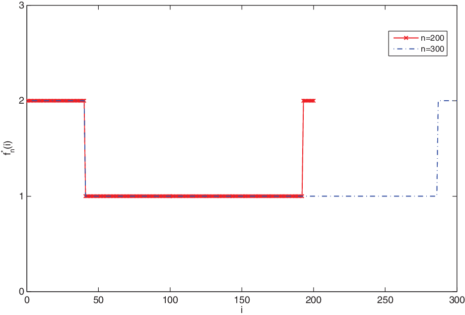
- $n=200$: $f^*_n(0)=\alpha_2$, $f^*_n(i)=\{0\} \times\{\mu\}$ for $i=1,\ldots,40$, $f^*_n(i)=\{0\} \times\{0\}$ for $i=41,\ldots,192$, $f^*_n(i)=\{0\} \times\{\mu\}$ for $i=193,\ldots,200$.
- $n=300$: $f^*_n(0)=\alpha_2$, $f^*_n(i)=\{0\} \times\{\mu\}$ for $i=1,\ldots,40$, $f^*_n(i)=\{0\} \times\{0\}$ for $i=41,\ldots,286$, $f^*_n(i)=\{0\} \times\{\mu\}$ for $i=287,\ldots,300$.





To see the numerical results more clearly, we plot the optimal policies  $f^*_n$ for
 $n=200$ and
 $n=300$ in Figure 1, where the symbols 1,2,3,4 represent the actions
 $\{0\}\times \{0\}$,
 $\{0\}\times \{\mu\}$,
 $\{\lambda\}\times \{0\}$,
 $\{\lambda\}\times \{\mu\}$, respectively.
Optimal policies.

Appendix A. Proofs
In this appendix we provide the proofs of Theorems 3.1 and 4.1, as well as Lemmas 3.1 and 3.2, which require the following lemma.
Lemma A.1. (Extension of Feynman–Kac formula.) Under Assumptions 3.1 and 3.2, for any  $T>0$ the following assertions hold, where
 $c(i,\pi_v)\,:\!=\,\int_{A(i)}c(i,a)\pi_v(\textrm{d} a \mid i)$ and
 $q(\,j \mid i,\pi_t)\,:\!=\,\int_{A(i)}q(\,j \mid i,a)\pi_t(\textrm{d} a \mid i)$ for
 $i,j\in S$,
 $t\geq 0$.
(a) For any
$\pi\in\Pi$ and $u\in \mathbb{B}_{V_0,V_1}^{ac}([0,T]\times S)$,
\begin{align*} & \mathbb{E}_{\gamma}^{\pi}\Bigg[\int_{0}^{T\wedge \tau_D} \Bigg(\frac{\partial\Big(\exp\left\{\int_0^t \int_A c(x_v,a)\pi(\textrm{d} a \mid \omega,v) \, \textrm{d} v\right\}u(t,x_t)\Big)}{\partial t} \\
& \qquad \qquad \qquad + \sum_{j\in S} \exp\left\{\int_0^t \int_A c(x_v,a)\pi(\textrm{d} a \mid \omega,v) \, \textrm{d} v\right\}u(t,j) \\
& \qquad \qquad \qquad \qquad \qquad \qquad \times \int_{A} q(\,j \mid x_t,a)\pi(\textrm{d} a \mid \omega,t)\Bigg) \, \textrm{d} t \, \big| \, x_0=i\Bigg ] \\
&\!\!\!\!\qquad = \mathbb{E}_\gamma^{\pi}\left[\exp\left\{\int_0^{T\wedge \tau_D} \int_A c(x_v,a)\pi(\textrm{d} a \mid \omega,v) \, \textrm{d} v\right\} u(T\wedge\tau_D,x_{T\wedge \tau_D}) \, \big| \, x_0=i\right]-u(0,i), \end{align*}
$i\in S, D\subseteq S$, where $\{x_t,t\geq 0\}$ may be not Markovian since the policy $\pi$ may depend on histories.
-
(b) For each
$\pi=\pi_t(\textrm{d} a \mid \cdot)\in\Pi_{m}^\textrm{r}$ and $u\in \mathbb{B}_{V_0,V_1}^{ac}([0,T]\times S)$,
for all
\begin{align*} & \mathbb{E}_{\gamma}^{\pi}\Bigg[\int_{s}^{T\wedge \tau_D} \Bigg(\frac{\partial\left(\exp\left\{\int_s^t c(x_v,\pi_v) \, \textrm{d} v\right\}u(t,x_t)\right)}{\partial t} \\
& \qquad \qquad \qquad + \sum_{j\in S}\left(\exp\left\{\int_s^t c(x_v,\pi_v) \, \textrm{d} v\right\}u(t,j)\right)q(\,j \mid x_t,\pi_t)\Bigg) \, \textrm{d} t \mid x_s=i\Bigg] \\
& \qquad = \mathbb{E}_{\gamma}^{\pi}\left[\exp\left\{\int_s^{T\wedge \tau_D} c(x_v,\pi_v) \, \textrm{d} v\right\}u(T\wedge \tau_D,x_{T\wedge \tau_D}) \mid x_s=i\right]-u(s,i) \end{align*}
$(s,i)\in [0,T]\times S$, $D\subseteq S$.


Proof. By Assumption 3.1(iii), we have  $2tc(i,a)\leq 2t\delta(i)\leq 2t\sqrt{\ln V_0(i)} \leq t^2+\ln V_0(i)$ for all
 $t\geq 0$, and thus
 $\textrm{e}^{2Tc(i,a)}\leq \textrm{e}^{T^2}V_0(i)$ for all
 $i\in S$, which verifies Assumption 3.1(iii) with
 $M_0\,:\!=\,\textrm{e}^{T^2}$ in [Reference Guo, Liu and Zhang9]. Thus, from the proof of [Reference Guo, Liu and Zhang9, Theorem 3.1], replacing T with
 $T\wedge \tau_D$, we see that this lemma is also true.
A.1. Proof of Lemma 3.1
(a) Obviously, the results hold for
$i=i_0$. For any $i \not=i_0$, since $V_0\geq 1$, by Lemma A.1(a) for $u\,:\!=\,V_0$ and $c(i,\cdot)\,:\!=\,\delta(i)$ we have
which, together with letting
\begin{align*} & \mathbb{E}_{i}^{\pi}\left[\exp\left\{\int_0^{T\wedge \tau_{i_0}}\!\!\delta(x_v) \, \textrm{d} v\right\}\right]-V_0(i) \leq \mathbb{E}_{i}^{\pi}\left[\exp\left\{\int_0^{T\wedge \tau_{i_0}}\!\!\delta(x_v) \, \textrm{d} v\right\}V_0\big(x_{T\wedge \tau_{i_0}}\big)\right]-V_0(i) \\
& \qquad = \mathbb{E}_{i}^{\pi}\bigg[\int_{0}^{T\wedge \tau_{i_0}}\exp\bigg\{\int_0^t\delta(x_v) \, \textrm{d} v\bigg\} \bigg(\delta(x_t)V_0(x_t)+\sum_{j\in S}V_0(\,j)q(\,j \mid x_t,\pi_t)\bigg) \textrm{d} t\bigg] \\
& \qquad \leq b_0\mathbb{E}_{i}^{\pi}\bigg[\int_{0}^{T\wedge \tau_{i_0}}\exp\bigg\{\int_0^t\delta(x_v) \, \textrm{d} v\bigg\}\mathbf{1}_{\{i_0\}}(x_t) \, \textrm{d} t\bigg]=0,\end{align*}
$T\to\infty$, gives the desired result.
-
(b) Since
$\delta_*=\inf_{i\not=i_0}\delta(i)>0$, by (a) and the Jensen inequality, we have
which implies (b).
\begin{eqnarray*} \delta_*\mathbb{E}_{i}^{\pi}[\tau_{i_0}]\leq \textrm{e}^{\delta_*\mathbb{E}_{i}^{\pi}[\tau_{i_0}]} \leq \mathbb{E}_{i}^{\pi} \left[\exp\left\{\int_0^{\tau_{i_0}}\delta(x_v) \, \textrm{d} v\right\}\right] \leq V_0(i),\end{eqnarray*}


A.2 Proof of Theorem 3.1
(a) Since Assumption 3.1(iii) in [Reference Guo, Liu and Zhang9] has been verified in the proof of Lemma A.1, for any
$i \in S$, by [Reference Guo, Liu and Zhang9, Theorem 4.1] and an obvious change of time, we have
Furthermore, for any
\begin{eqnarray*} \begin{cases} \varphi'(t,i)=\inf_{a\in A(i)}\left[c(i,a)\varphi(t,i)+\sum_{j\in S}\varphi(t,j)q(\,j \mid i,a)\right] \text{almost surely for} \ t \in [0,T], \\ \varphi(0,i)=1. \end{cases}\end{eqnarray*}
$t_1,t_2\in [0,T]$, $\varepsilon>0$, Assumption 3.3 together with [Reference Guo, Huang and Huang15, Lemma 4.1] ensures the existence of $a(i,t_1,t_2)\in A(i)$ and a finite subset S(i) of S (depending on i) such that $i\in S(i)$ and $\sup_{a\in A(i)}\sum_{j\not\in S(i)}|\varphi(t_1,j)-\varphi(t_2,j)||q(\,j \mid i,a)|=\sum_{j\not\in S(i)}|\varphi(t_1,j)-\varphi(t_2,j)||q(\,j \mid i,a(i,t_1,t_2))|$, and $\sum_{j\not\in S(i)}V_0(\,j)q(\,j \mid i,a)<\varepsilon$ for all $a\in A(i)$. Thus, for any $t_1,t_2\in [0,T]$, we have
which, together with the continuity of
\begin{align*} \|c(i,\cdot)\| |\varphi(t_1, & i) - \varphi(t_2,i)|+\sup_{a\in A(i)}\sum_{j\in S}|\varphi(t_1,j)-\varphi(t_2,j)||q(\,j \mid i,a)| \\ & \leq \|c(i,\cdot)\| |\varphi(t_1,i)-\varphi(t_2,i)|+\sum_{j\in S(i)}|\varphi(t_1,j)-\varphi(t_2,j)|q^*(i) \\ & \quad + 2\|\varphi\|_{V_0} \sum_{j\not\in S(i)}V_0(\,j)q(\,j \mid i,a(i,t_1,t_2)) \\ & \leq \|c(i,\cdot)\| |\varphi(t_1,i)-\varphi(t_2,i)|+\sum_{j\in S(i)}|\varphi(t_1,j)-\varphi(t_2,j)|q^*(i)+2\|\varphi\|_{V_0}\varepsilon,\end{align*}
$\varphi(t,i)$ in t and the finiteness of $\|c(i,\cdot)\|, S(i)$ and $q^*(i)$, implies that $\inf_{a\in A(i)}[c(i,a)\varphi(t,i)+\sum_{j\in S}\varphi(t,j)q(\,j \mid i,a)]$ is continuous in $t\geq 0$ for any fixed $i\in S$. Hence, by the first equation in this proof, $\varphi'(t,i)$ exist for all $t\geq 0$ and $\varphi'(t,i)$ is continuous in $t\geq 0$.
-
(b) follows from Theorem 4.2(c) in [Reference Guo, Liu and Zhang9].
-
(c) Let
$\pi=f_t$ be any Markov policy in $\Pi_\textrm{m}^\textrm{d}$, and $\pi^*=f^\ast_t$ the deterministic Markov policy from part (b). Define a policy $\hat{\pi}$ by $\hat{\pi}(\textrm{d} a \mid \omega,s) = \mathbf{1}_{\{t\wedge \tau_D > s\}} \delta_{f_s(x_s(\omega))}(\textrm{d} a)+\mathbf{1}_{\{t\wedge \tau_D\leq s\}}\delta_{f^\ast_s(x_s(\omega))}(\textrm{d} a)$. Let ${\mathcal{F}}_{t\wedge \tau_D}$ be the $\sigma$-algebra generated by the stopping time $t\wedge \tau_D$ with respective the filtration ${\mathcal{F}}_s\,:\!=\,\sigma(x_v,v\leq s)$. Since $\varphi(t,i)= \varphi(t,i,\pi^*)$ for $t\in [0,T]$ and $i\in S$, we have
Taking the infimum over
\begin{align*} \varphi(t,i) & \leq \mathbb{E}_i^{\hat{\pi}}\left[\exp\left\{\int_0^{t} \int_A c (x_s,a)\hat{\pi}(\textrm{d} a \mid \omega,s) \, \textrm{d} s\right\} \right] \\[3pt]
& = \mathbb{E}_i^{\hat\pi}\left[\exp\left\{\int_0^{t\wedge \tau_D}c(x_s,f_s(x_s)) \, \textrm{d} s\right\} \mathbb{E}_i^{\hat\pi}\left[\exp\left\{\int_{t\wedge \tau_D}^t c(x_s,f_s(x_s)) \, \textrm{d} s\right\} \, \big| \, {\mathcal{F}}_{t\wedge \tau_D}\right]\right] \\[3pt]
& = \mathbb{E}_i^{\pi}\left[\exp\left\{\int_0^{t\wedge \tau_D} c(x_s,f_s(x_s)) \, \textrm{d} s\right\}\varphi(t-t\wedge \tau_D,x_{t\wedge \tau_D},\pi^*)\right] \\[3pt] & = \mathbb{E}_i^{\pi}\left[\exp\left\{\int_0^{t\wedge \tau_D} c(x_s,f_s(x_s)) \, \textrm{d} s\right\}\varphi(t-t\wedge \tau_D,x_{t\wedge \tau_D})\right] \\[3pt] & \leq \mathbb{E}_i^{\pi}\left[\exp\left\{\int_0^{t\wedge \tau_D} c(x_s,f_s(x_s)) \, \textrm{d} s\right\}\varphi(t-t\wedge \tau_D,x_{t\wedge \tau_D},\pi)\right]=\varphi(t,i,\pi).\end{align*}
$\pi\in\Pi_\textrm{m}^\textrm{d}$ on both sides of the above inequality and using (b) again, we see that part (c) holds.





A.3 Proof of Lemma 3.2
(a) Since
$1=\varphi(0,i)\leq \varphi(t,i)$ for all $i\in S$ and $t\geq 0$, by Theorem 3.1(c) we have, for each $\pi\in \Pi$,which, together with Lemma 3.1(a), completes the proof of part (a).
\fontsize{9.6}{10.8}\selectfont{\begin{align*} \varphi(t,i) & \leq \mathbb{E}_i^{\pi}\left[\exp\left\{\int_0^{t\wedge \tau_{i_0}}c(x_v,\pi_v) \, \textrm{d} v\right\}\varphi (t-t\wedge \tau_{i_0},x_{t\wedge \tau_{i_0}})\right] \\[3pt]
& = \mathbb{E}_i^{\pi}\left[\exp\left\{\int_0^{t\wedge \tau_{i_0}}c(x_v,\pi_v) \, \textrm{d} v\right\}\varphi (t-t\wedge \tau_{i_0},x_{t\wedge \tau_{i_0}})\mathbf{1}_{\{t\leq \tau_{i_0}\}}\right] \\[3pt]
& \quad + \mathbb{E}_i^{\pi}\left[\exp\left\{\int_0^{t\wedge \tau_{i_0}}c(x_v,\pi_v) \, \textrm{d} v\right\}\varphi (t-t\wedge \tau_{i_0},x_{t\wedge \tau_{i_0}})\mathbf{1}_{\{t>\tau_{i_0}\}}\right] \\[3pt]
& = \mathbb{E}_i^{\pi}\left[\exp\left\{\int_0^{t\wedge \tau_{i_0}}c(x_v,\pi_v) \, \textrm{d} v\right\}\mathbf{1}_{\{t\leq \tau_{i_0}\}}\right] \\[3pt]
& \quad + \mathbb{E}_i^{\pi}\left[\exp\left\{\int_0^{t\wedge \tau_{i_0}}c(x_v,\pi_v) \, \textrm{d} v\right\}\varphi (t-\tau_{i_0},x_{\tau_{i_0}})\mathbf{1}_{\{t>\tau_{i_0}\}}\right] \\[3pt]
& \leq \mathbb{E}_i^{\pi}\left[\exp\left\{\int_0^{t\wedge \tau_{i_0}}c(x_v,\pi_v) \, \textrm{d} v\right\}\varphi (t,x_{\tau_{i_0}})\mathbf{1}_{\{t\leq \tau_{i_0}\}}\right] \\[3pt]
& \quad + \mathbb{E}_i^{\pi}\left[\exp\left\{\int_0^{t\wedge \tau_{i_0}}c(x_v,\pi_v) \, \textrm{d} v\right\}\varphi (t,x_{\tau_{i_0}})\mathbf{1}_{\{t>\tau_{i_0}\}}\right] \\[3pt]
& \leq \mathbb{E}_i^{\pi}\left[\exp\left\{\int_0^{\tau_{i_0}}c(x_v,\pi_v) \, \textrm{d} v\right\}\varphi (t,x_{\tau_{i_0}})\right] \\[3pt]
& = \varphi (t,i_0)\mathbb{E}_i^{\pi}\left[\exp\left\{\int_0^{\tau_{i_0}}c(x_v,\pi_v) \, \textrm{d} v\right\}\right], \nonumber\end{align*}}
-
(b)
$\varphi(t,i)$ is increasing in t for each $i\in S$, and thus $\varphi'(t,i)\geq 0$. Moreover, for each $t\geq 0$, by (a) and Assumption 3.1(i) we have
and so part (b) follows.
\begin{align*} 0 \leq \frac{\varphi'(t,i)}{\varphi(t,i_0)} & = \inf_{a\in A(i)}\bigg[c(i,a) \frac{\varphi(t,i)}{\varphi(t,i_0)}+\sum_{j\in S}\frac{\varphi(t,j)}{\varphi(t,i_0)}q(\,j \mid i,a)\big] \\
& \leq \inf_{a\in A(i)}\bigg[\delta(i)V_0(i)+\sum_{j\in S}V_0(\,j)|q(\,j \mid i,a)|\bigg] \\ & = \inf_{a\in A(i)}\bigg[\delta(i)V_0(i)+\sum_{j\in S}V_0(\,j)q(\,j \mid i,a)-2q(i \mid i,a)V_0(i)\bigg] \\ & \leq 2q^*(i)V_0(i)+b_0 , \end{align*}


A.4 Proof of Theorem 4.1
As in the arguments in [Reference Kumar and Pal23], we prove Theorem 4.1 by Theorem 3.2 and Lemma 3.2.
(a) For any fixed
$n\geq 1$, and for $t \geq 0$, $i \in S$, let
(24)Then, since
\begin{eqnarray} \varphi_n(t,i)\,:\!=\,\inf_{\pi\in\Pi^\textrm{d}_\textrm{m}} \mathbb{E}_i^{\pi}\left[\exp\left\{\int_0^tc_n(x_v,\pi_v) \, \textrm{d} v\right\}\right] (\geq 0), \quad \hat\varphi_n(t,i)\,:\!=\,\frac{\varphi_n(t,i)}{\varphi_n(t,i_0)}. \end{eqnarray}
$0\leq c_n\leq c$, the conditions of Theorem 3.1 and Lemma 3.2 still hold when c is replaced with $c_n$. Thus, using Lemma 3.2(a) and (24), we have $0 \leq \hat\varphi_n(t,i) \leq V_0(i)$ for all $t \geq 0$. Thus, for any $m\geq 1$, the mean value theorem together with Theorem 3.1(a) gives the existence of $k_0(i,m)\in [m,2m]$ (depending on the given m and i) such that
(25)Since S is denumerable, diagonalization arguments as well as (25) ensure the existence of a subsequence
\begin{eqnarray}\hat\varphi_n'(k_0(m,i),i)=\frac{\hat\varphi_n(2m,i)-\hat\varphi_n(m,i)}{2m-m}\to 0 \qquad (\textrm{as} \ m\to\infty). \end{eqnarray}
$\{k_1\}$ of $\{k_0(i,m),m\geq 1,i\in S\}$ such that $\lim_{k_1\to\infty}\hat\varphi_n'(k_1,i)=0$, $\hat\varphi_n(k_1,i_0)\equiv 1$ for all $i\in S$, which, together with the boundedness of $|\hat\varphi_n(k_1,i)|$ in $k_1$ and the denumerability of $i\in S$, gives the existence of a subsequence $\{k_2\}$ of $\{k_1\}$ such that the limits
(26)exist for all
\begin{eqnarray} \lim_{k_2\to\infty}\hat\varphi_n(k_2,i)=:\psi_n(i)\in [0,V_0(i)] \end{eqnarray}
$i\in S$, and $\psi_n(i_0)=1$.
Furthermore, Lemma 3.2(b) together with (26) guarantee the existence of a subsequence
$\{k_3\}$ of $\{k_2\}$ ensuring the existence of the limit
(27)Hence, along the sequence
\begin{eqnarray} \lim_{k_3\to\infty} \frac{\varphi_n'(k_3,i_0)}{\varphi_n(k_3,i_0)}=:\rho_n \in [0,L(i_0)]. \end{eqnarray}
$\{k_3\}$ $(\subset\{k_2\}\subset\{k_1\}\subset \{k_0(i,m),m\geq 1,i\in S\})$, we have
(28)On the other hand, for any number
\begin{eqnarray} \lim_{k_3\to\infty}\left[\hat\varphi_n'(k_3,i)+\hat\varphi_n(k_3,i)\frac{\varphi_n'(k_3,i_0)}{\varphi_n(k_3,i_0)}\right]=\rho_n \psi_n(i) \qquad \text{for all} \ i\in S. \end{eqnarray}
$k_3$ in the sequence $\{k_3\}$, using the definition of $\hat\varphi_n(t,i)$ in (24) and Theorem 3.1(a) with $(c, \varphi)$ replaced with the corresponding $(c_n,\varphi_n)$, direct calculation gives
(29)which, together with the dominated convergence theorem and (26)–(28), imply
\begin{align} &\hat\varphi_n'(k_3,i)+ \hat\varphi_n(k_3,i)\frac{\varphi_n'(k_3,i_0)}{\varphi_n(k_3,i_0)} = \inf_{a\in A(i)}\bigg\{ c_n(i,a)\hat\varphi_n(k_3,i)+\sum_{j\in S}\hat\varphi_n(k_3,j)q(\,j \mid i,a)\bigg\}\nonumber\\
&\quad \leq c_n(i,a)\hat\varphi_n(k_3,i)+\sum_{j\in S}\hat\varphi_n(k_3,j)q(\,j \mid i,a) \qquad \text{for all} \ (i,a)\in K,
\end{align}
Moreover, for each given
\begin{eqnarray*} \rho_n \psi_n(i)\leq \inf_{a\in A(i)}\bigg\{ c_n(i,a)\psi_n(i)+\sum_{j\in S}\psi_n(\,j)q(\,j \mid i,a)\bigg\} \qquad \text{for all} \ i\in S. \end{eqnarray*}
$k_3$ and $i\in S$, by Assumption 3.3 and (28), there exists $a(i,k_3)\in A(i)$ (depending on $k_3, i\in S$) such that
(30)Since A(i) is compact, there exist a subsequence
\begin{align} & \hat\varphi_n'(k_3,i)+\hat\varphi_n(k_3,i)\frac{\varphi_n'(k_3,i_0)}{\varphi_n(k_3,i_0)}\nonumber\\
& \qquad =c_n(i,a(i,k_3))\hat\varphi_n(k_3,i)+\sum_{j\in S}\hat\varphi_n(k_3,j)q(\,j \mid i,a(i,k_3)). \end{align}
$\{k_4\}$ of $\{k_3\}$ and $a'(i)\in A(i)$ such that $\lim_{k_4\to\infty} a(i,k_4)=a'(i)$. Thus, replacing $k_3$ in (30) with $k_4$ and then letting $k_4\to\infty$, by (28) and (30) we have
which, together with (29), (26), and (27), gives (a).
\begin{align*} \rho_n \psi_n(i) & = c_n(i,a'(i))\psi_n(i)+\sum_{j\in S}\psi_n(\,j)q(\,j \mid i,a'(i)) \\ & \geq \inf_{a\in A(i)}\bigg\{ c_n(i,a)\psi_n(i)+\sum_{j\in S}\psi_n(\,j)q(\,j \mid i,a)\bigg\}, \end{align*}
-
(b) Fix any
$i\geq n+1$ with $n\geq i_0$, and let $\tau(n)\,:\!=\,\tau_{\{0,1,\ldots,i_0,\ldots,n\}}$ be the hitting time. Then, by Lemma 3.1(b) and $\tau(n)\leq \tau_{i_0}$, $\mathbb{P}_{i}^{\pi}(\tau(n)<\infty)=1$. Moreover, since $\varphi_n(0,i)\equiv 1$ and $\varphi_n(t,i)$ is increasing in $t\geq 0$, using (4) and Theorem 3.1(c) (with c replacing by $c_n$ here) as well as the fact that $c_n(x_v,\pi_v)\equiv0$ for $v<\tau(n)$, we have, for each $\pi\in \Pi$,
which, together with Lemma 3.2(a) and
\begin{align*} \varphi_n(t,i) & \leq \mathbb{E}_i^{\pi}\bigg[\exp\bigg\{\int_0^{t\wedge \tau(n)}c_n(x_v,\pi_v) \, \textrm{d} v\bigg\}\varphi_n(t-t\wedge \tau(n),x_{t\wedge \tau(n)})\bigg] \\[2pt]
& = \mathbb{E}_i^{\pi}\bigg[\exp\bigg\{\int_0^{t\wedge \tau(n)}c_n(x_v,\pi_v) \, \textrm{d} v\bigg\}\varphi_n(t-t\wedge \tau(n),x_{t\wedge\tau(n)})\mathbf{1}_{\{t\leq \tau(n)\}}\bigg] \\[2pt]
& \quad + \mathbb{E}_i^{\pi}\bigg[\exp\bigg\{\int_0^{t\wedge \tau(n)}c_n(x_v,\pi_v) \, \textrm{d} v\bigg\}\varphi_n(t-t\wedge \tau(n),x_{t\wedge\tau(n)})\mathbf{1}_{\{t>\tau(n)\}}\bigg] \\
& = \mathbb{E}_i^{\pi}\bigg[\varphi_n(0,x_t)\mathbf{1}_{\{t\leq\tau(n)\}}\bigg]+\mathbb{E}_i^{\pi}\bigg[\varphi_n(t-\tau(n),x_{\tau(n)})\mathbf{1}_{\{t>\tau(n)\}}\bigg] \\[2pt] & \leq 1+\mathbb{E}_i^{\pi}\bigg[\varphi_n(t,x_{\tau(n)})\mathbf{1}_{\{t>\tau(n)\}}\bigg] \\[2pt] & \leq 1+\max\{\varphi_n(t,k),k=0,1,\ldots,n\},\end{align*}
$\varphi_n\geq 1$, imply that $\hat\varphi_n(t,i)\leq 1+\max\{V_0(k), k=0,1,\ldots,n\}=:K(n)$ for all $t\geq 0$, $i\in S$. Hence, using (26) and Lemma 3.2(a) again, we have
(31)For each
\begin{eqnarray}\psi_n(i) \leq K(n) \qquad \text{for all} \ t\geq 0, i\in S. \end{eqnarray}
$\pi\in \Pi$ and $i\in S$, using Lemma A.1(a) and (5), we have
Hence, by (31) we have
\begin{eqnarray*} \mathbb{E}_{i}^{\pi}\left[\exp\left\{\int_{0}^{T}\int_{A}[c_n(x_t,a)-\rho_n]\pi(\textrm{d} a \mid \omega,t) \, \textrm{d} t\right\}\psi_n(x_T)\right]-\psi_n(i)\geq 0 \qquad \textrm{for } \ T>0.\end{eqnarray*}
Taking logarithms of both sides, dividing by T, and letting
\begin{eqnarray*} K(n)\textrm{e}^{-T\rho_n}\mathbb{E}_{i}^{\pi}\left[\exp\left\{\int_{0}^{T}\int_{A}c_n(x_t,a)\pi(\textrm{d} a \mid \omega,t) \, \textrm{d} t\right\}\right]\geq \psi_n(i).\end{eqnarray*}
$T\to\infty$, we obtain
which, together with the arbitrariness of
\begin{align*} \rho_n & \leq \limsup_{T\to\infty} \frac{1}{T}\ln\mathbb{E}_{i}^{\pi}\left[\exp\left\{\int_{0}^{T}\int_{A}c_n(x_t,a)\pi(\textrm{d} a \mid \omega,t) \, \textrm{d} t\right\}\right] \\[2pt] & \leq \limsup_{T\to\infty} \frac{1}{T}\ln\mathbb{E}_{i}^{\pi}\left[\exp\left\{\int_{0}^{T}\int_{A}c(x_t,a)\pi(\textrm{d} a \mid \omega,t) \, \textrm{d} t\right\}\right],\end{align*}
$\pi$, completes the proof of (b).
-
(c) For each
$\pi\in \Pi_\textrm{m}^\textrm{d}$ and $i\in S$, using Lemma A.1(b) and (5) again, we have
Since
\begin{eqnarray*} \mathbb{E}_{i}^{\pi}\left[\exp\left\{\int_{0}^{T\wedge\tau_{i_0}}(c_n(x_t,\pi_t)-\rho_n) \, \textrm{d} t\right\}\psi_n(x_{T\wedge \tau_{i_0}})\right]-\psi_n(i)\geq 0 \qquad \textrm{for} \ T>0.\end{eqnarray*}
$\psi_n$ is bounded and $c_n(i,a)\leq c(i,a)\leq \delta(i)$ for all $(i,a)\in K$, by the dominated convergence theorem and Lemma 3.1(a), letting $T\to\infty$, we obtain
(32)which, together with the arbitrariness of
\begin{align} \psi_n(i) & \leq \mathbb{E}_{i}^{\pi}\left[\exp\left\{\int_{0}^{\tau_{i_0}}[c_n(x_t,\pi_t)-\rho_n] \, \textrm{d} t\right\}\psi_n(x_{\tau_{i_0}})\right] \nonumber \\ & = \mathbb{E}_{i}^{\pi}\left[\exp\left\{\int_{0}^{\tau_{i_0}}[c_n(x_t,\pi_t)-\rho_n] \, \textrm{d} t\right\}\right]\leq V_0(i) , \end{align}
$\pi\in \Pi_\textrm{m}^\textrm{d}$, imply
(33)On the other hand, take
\begin{eqnarray} \psi_n(i) \leq \inf_{\pi\in\Pi_\textrm{m}^\textrm{d}} \mathbb{E}_{i}^{\pi}\left[\exp\left\{\int_{0}^{\tau_{i_0}}[c_n(x_t,\pi_t)-\rho_n] \, \textrm{d} t\right\}\psi_n(x_{\tau_{i_0}})\right]\leq V_0(i). \end{eqnarray}
$f^*_n\in F$ to be a minimizing stationary policy in (5), that is,
(34)Using Lemma A.1(b) and (34), as in the proof of (32) (by Fatou’s lemma again) we have
\begin{eqnarray} \rho_n\psi_n(i) = c(i,f^*_n(i))\psi_n(i)+\sum_{j\in S}\psi_n(\,j)q(\,j \mid i,f^*_n(i)) \qquad \text{for all} \ i\in S. \end{eqnarray}
This inequality, as well as (33), gives (c).
\begin{eqnarray*} \psi_n(i)\geq\mathbb{E}_{i}^{f^*_n}\left[\exp\left\{\int_{0}^{\tau_{i_0}}(c_n(x_t,f^*_n(x_t))-\rho_n) \, \textrm{d} t\right\}\right].\end{eqnarray*}








Remark A.1. In order to establish the existence of  $k_0(m,i)$ for (25) to hold, the existence of
 $\varphi'(t,i)$ for the function
 $\varphi(t,i)$ at each
 $t\geq 0$ is required. Otherwise, such
 $k_0(m,i)$ cannot be guaranteed. For example, for some given
 $i\in S$ and
 $n\geq 1$, suppose that
 \begin{eqnarray*} \hat\varphi_n(t,i)\,:\!=\, \begin{cases} t+1, & t\in [1,1.5), \\ 4-t, & t\in [1.5,2]. \end{cases} \end{eqnarray*}
Take  $m=1$. Then,
 $\frac{\hat\varphi_n(2,i)-\hat\varphi_n(1,i)}{2-1}=0\not= \hat\varphi_n'(k_0(1,i),i)$ for any
 $k_0(1,i)\in[1,2]$.
Acknowledgements
Research supported by the National Natural Science Foundation of China (grant nos. 11931018, 61773411, 11961005) and Guangdong Province Key Laboratory of Computational Science at the Sun Yat-Sen University (2020B1212060032).