



1. Introduction
1.1. Motivation
In this paper we study the well-known ruin problem for insurance companies investing their reserves in financial markets. Such problems were first considered for the Cramér–Lundberg model (see, for example, [Reference Mikosch18, Section 4] and the references therein) in which the surplus process is defined by the equality
 \begin{equation}{\mathbf{J}^{u}_{t}}=u+ct-\sum^{N_{t}}_{j=1} \xi_{j},\end{equation}
where
 $u>0$
is the initial capital,
 $c>0$
the premium rate,
 $N=(N_t)_{t\ge 0}$
a homogeneous Poisson process, and the claim sizes
 $(\xi_j)_{j\ge 1}$
are i.i.d. (independent and identically distributed) non-negative RVs (random variables). The classical condition to avoid ruin is that the rate c has to be more than some positive threshold (the net profit condition). Note that if this condition does not hold, then the company will suffer ruin almost surely. So, a natural question arises as to what should be done in this case. To avoid almost sure ruin, [Reference Frolova, Kabanov and Pergamenshchikov8] proposed that insurance companies invest their reserves in Black–Scholes markets. In this case, it turns out that the condition providing the decay of the ruin probability to 0 depends only on the market parameters and not on the premium rate c. Moreover, as shown in [Reference Pergamenshchikov and Zeitouni23], even for
 $c=0$
the ruin probability goes to 0 with the same power rate as for
 $c>0$
, i.e. the asymptotic form of the ruin probability depends only on the market coefficients. Later, in [Reference Eberlein, Kabanov and Schmidt6], ruin problems for insurance companies with investments were studied for a more general insurance context defined by the Sparre–Andersen models (see, for example, [Reference Back, Bielecki, Hipp, Peng and Schachermayer3, Reference Sparre Andersen25] and the references therein) in which the claim number process
 $N=(N_t)_{t\ge 0}$
is general renewal counting defined as
 \begin{align}N_{t}=\sum_{n\ge 1} \mathbf{1}_{\{\mathbf{t}_{n}\le t\}}, \qquad \mathbf{t}_{n}=\sum^{n}_{j=1}\tau_{j},\end{align}
where
 $\mathbf{1}_{A}$
is the indicator of the set A and
 $(\tau_{j})_{j\ge 1}$
are i.i.d. RVs. Note that if
 $(\tau_{j})_{j\ge 1}$
are exponential, then
 $(N_{t})_{t\ge 0}$
is a homogeneous Poisson process. For a non-exponential distribution the process
 $(N_{t})_{t\ge 0}$
has dependent increments. This is the main difficulty that arises when studying this model. If a company invests its reserve in the Black–Scholes markets, i.e. it uses geometric Brownian motion to describe price dynamics, there is the possibility of avoiding working directly with the process
 $(N_{t})_{t\ge 0}$
by considering the surplus process only in the jump moments
 $(\mathbf{t}_{n})_{n\ge 1}$
in which
 $N_{\mathbf{t}_{n}}=n$
and the increments of the logarithm price process on the intervals
 $(\mathbf{t}_{n-1},\mathbf{t}_{n})$
are independent (see [Reference Eberlein, Kabanov and Schmidt6] for the details). However, this approach does not work for more complex price processes with dependent logarithmic increments, such as stochastic volatility markets with Markov switching. For such settings, the ruin problem has been studied only for the Cramér–Lundberg model (1.1), i.e. in the case when
 $N_{t}$
is the Poisson process (see, for example, [Reference Ellanskaya and Kabanov7, Reference Kabanov and Pergamenshchikov12, Reference Palmowski19, Reference Ramsden and Papaioannou24] and the references therein). The question about the asymptotic form of the ruin probability for general non-exponential RVs
 $(\tau_{j})_{j\ge 1}$
is open. It should be emphasized that in practice, the more natural case is when the RVs
 $(\tau_{j})_{j\ge 1}$
are non-exponential but bounded, for example uniformly distributed.
1.2. Main contributions
The goal is to study the behavior of an insurance company within the framework of Sparre–Andersen models under investments in financial markets with functional coefficients defined through hidden Markov chains. Usually, ruin problems are studied through Goldie’s results on the asymptotic behavior of the tail of the solutions of random equations. The main condition of Goldie’s theorem is the independence of the coefficients in these equations from their solutions (see, for example, [Reference Eberlein, Kabanov and Schmidt6, Reference Ellanskaya and Kabanov7, Reference Kabanov and Pergamenshchikov11, Reference Kabanov and Pergamenshchikov12, Reference Paulsen22] and the references therein). This condition holds either for the Cramér–Lundberg model with investments in stochastic volatility models or for the Sparre–Andersen model with investments in Black–Scholes markets. Unfortunately, Goldie’s method cannot be applied to study ruin problems within the framework of Sparre–Andersen models when investing in stochastic volatility markets, since in this case the solution of the corresponding random underlying equation depends on its coefficients through a hidden Markov chain governing the market coefficients. In this paper, to study this problem we develop a new method based on the key renewal theorem shown in [Reference Klüppelberg and Pergamenchtchikov15] for general Markov chains. This approach allows us to take into account the influence of Markov chains on the dynamics of capital and to study the asymptotic property of the solution of the corresponding basic random equation in the case where the conditions of Goldie’s theorem are not met. As a result, constructive conditions for market coefficients are found, under which the probability of ruin tends to zero with a power rate. The developed method extends and complements the results obtained for stochastic volatility models in [Reference Ellanskaya and Kabanov7, Reference Kabanov and Pergamenshchikov12]. More precisely, this paper shows for the first time that the asymptotic power form is the same for all initial states of the Markov chain. This effect was discovered for two-state Markov chains in [Reference Ellanskaya and Kabanov7], but in the general case, i.e. for chains with any arbitrary number of states, this question was open even for the Cramér–Lundberg model [Reference Kabanov and Pergamenshchikov12]. Next, investment strategies are constructed for which the power of the convergence rate for the ruin probability is explicitly calculated, and, moreover, conditions are found under which this degree can be arbitrarily large, i.e. the ruin probability decays to zero more rapidly than any power function.
1.3. Organization of the paper
In Section 2 we describe the insurance model and state the ruin problem. In Section 3 the main conditions are given. In Section 4 the main asymptotic results on ruin probabilities are stated. In Section 5 we study the renewal operator, which plays a crucial role in the renewal analysis methods described in Section 7. Section 6 presents the key renewal theorem from [Reference Klüppelberg and Pergamenchtchikov15]. All the main results are proved in Section 8. The results of the Monte Carlo simulations are given in Section 9. Concluding remarks are given in Section 10. Some auxiliary analytic tools are presented in Appendix A.
2. Model
In the present paper we study the behavior of insurance companies in the framework of the Sparre–Andersen version model (see, for example, [Reference Asmussen and Albrecher2, Chapter VIII, Section 6]), i.e. its surplus process is defined as
 \begin{equation} {\mathbf{J}^{u}_{t}}=u- \sum_{k=1}^{N_{t}}\xi_{k},\end{equation}
where
 $u>0$
is the initial capital of the company,
 $(\xi_{k})_{k \ge 1}$
is a sequence of i.i.d. RV’s (probably two-sided RVs) which can be represented as
 $\xi_{k}=\xi^{+}_{k}-\xi^{-}_{k}$
, with their positive part
 $\xi^{+}_{k}=\max(\xi_{k},0)$
and the negative one
 $\xi^{-}_{k}=-\min(\xi_{k},0)$
, and
 $(N_{t})_{t\ge 0}$
is the renewal counting process defined in (1.2). This model includes two different cases:
 $\xi^{-}_{k}= 0$
almost surely (a.s.), i.e. the Sparre–Andersen model (1.1) with
 $c=0$
, and the pure Sparre–Andersen model when
 ${\mathbb P}(\xi^{-}_{k} > 0) > 0 $
. In addition, we consider insurance companies investing their reserves in a Black–Scholes market with a risk-free asset
 $B_{t}\equiv 1$
and a risky asset defined by the stochastic differential equation
 \begin{equation}\mathrm{d} S_{t}=S_{t} (a_{0,t}\,\mathrm{d} t+\sigma_{0,t}\,\mathrm{d} W_{t}), \qquad S_{0}=1,\end{equation}
in which the coefficients
 $a_{0,t}=a_{0}(\theta_{t})$
and
 $\sigma_{0,t}=\sigma_{0}(\theta_{t})$
are functions of an external random source specified by a homogeneous irreducible stationary Markov càdlàg process
 $(\theta_{t})_{t\ge 0}$
with values in the finite set
 $\mathcal{X}=\{\kappa_{1},\ldots,\kappa_{d}\}$
. We assume that its stationary distribution
 $\pi$
is strictly positive, i.e.
 \begin{equation} \min_{x\in \mathcal{X}} \pi(x) >0 .\end{equation}
The company investment portfolio
 $(\beta_{s},\gamma_{s})_{s\ge 0}$
is a financial strategy in which the first component,
 $\beta_{s}$
, is the number of risk-free assets and the second.
 $\gamma_{s}$
, is the number of risky assets at the time
 $s\ge0$
. Using in the insurance model the self-financial consumption principle (see, for example, [Reference Karatzas and Shreve13, Chapter 3]), the corresponding surplus process (2.1) can be rewritten as
 \begin{align*} X^{u}_{t}=\beta_{t}+\gamma_{t}S_{t} =u+\int^{t}_{0}\gamma_{s}\,\mathrm{d} S_{s}- \sum_{k=1}^{N_{t}} \xi_{k}. \end{align*}
Introducing here the fractional strategy
 $\widehat{\gamma}_{t}=\gamma_{t}S_{t}/X_{t}$
and using (2.2), we get
 \begin{equation} X^{u}_{t}=u+ \int_{0}^{t} \mathbf{a}_{s}X^{u}_{s}\,\mathrm{d} s + \int_{0}^{t} \sigma_{s} X^{u}_{s}\,\mathrm{d} W_{s} - \sum_{k=1}^{N_{t}} \xi_{k} ,\end{equation}
where
 $\mathbf{a}_{s}=a_{0,s}\widehat{\gamma}_{s}$
and
 $\sigma_{s}=\sigma_{0,s}\widehat{\gamma}_{s}$
. For fractional strategies of the form
 $\widehat{\gamma}_{s}=\widehat{\gamma}(\theta_{s})$
the coefficients
 $\mathbf{a}_{s}$
and
 $\sigma_{s}$
are functions of the chain
 $(\theta_{t})_{t\ge 0}$
, i.e.
 \begin{equation} \mathbf{a}_{s} = \mathbf{a}(\theta_{s}) =a_{0}(\theta_{s})\widehat{\gamma}(\theta_{s}), \qquad\sigma_{s}=\sigma(\theta_{s})=\sigma_{0}(\theta_{s})\widehat{\gamma}(\theta_{s}).\end{equation}
In this paper we consider ruin problems for the model (2.4). At first, for any
 $u>0$
we define the moment of the company’s ruin as
 \begin{equation} \upsilon_{u}\, :\!= \,\inf \{t>0\colon X^{u}_t\le 0\}\end{equation}
and the ruin probabilities as
 \begin{equation} \Psi(u)\, :\!= \,{\mathbb P}(\upsilon_{u} < \infty), \qquad \Psi(u,x)\, :\!= \,{\mathbb P}_{x}(\upsilon_{u} < \infty) ,\end{equation}
where
 ${\mathbb P}_{x}(\cdot)$
is the probability distribution under the condition that
 $\theta_{0}=x$
. It is clear that
 \begin{equation} \Psi(u)=\sum_{x\in\mathcal{X}}\,\Psi(u,x)\pi(x).\end{equation}
The main purpose is to study the asymptotic behavior of the function
 $\Psi(u)$
when
 $u\to+\infty$
. Similarly to [Reference Ellanskaya and Kabanov7, Reference Kabanov and Pergamenshchikov12], to provide the decay of the function
 $\Psi(u)$
to zero, we need to assume that the coefficients in the market (2.2),
 $\mathbf{a}$
and
 $\sigma$
, are some
 $\mathcal{X}\to{\mathbb R}$
functions such that
 $\sigma_{*}=\min_{x\in\mathcal{X}}\sigma(x)>0$
and
 \begin{equation}\rho_{*}=\inf_{x\in\mathcal{X}}\rho(x)>0\quad\mbox{with}\quad\rho(x)=\frac{2\mathbf{a}(x)}{\sigma^{2}(x)}-1.\end{equation}
To study the ruin moment
 $\upsilon_{u}$
we represent the solution of the linear equation (2.4) in the form
 \begin{equation}X_t^{u}={\mathrm{e}}^{V_{t}}(u-Y_{t}), \qquad Y_{t}\, :\!= \,\int_{[0,t]}{\mathrm{e}}^{-V_{s}}\,\mathrm{d}\sum_{k=1}^{N_{s}} \xi_{k},\end{equation}
where
 \begin{align*} V_{t}= \int_{[0,t]} \widetilde{\mathbf{a}}_{s}\,\mathrm{d} s +\int_{[0,t]} \sigma_{s}\,\mathrm{d} W_{s}, \qquad \widetilde{\mathbf{a}}_{s}= \widetilde{\mathbf{a}}(\theta_{s}) =\mathbf{a}(\theta_{s})- \frac{\sigma^2(\theta_{s})}{2}. \end{align*}
It is clear that the moment (2.6) can be rewritten as
 $\upsilon_{u}= \inf \{t\ge 0\colon Y_{t} \ge u\}$
, and therefore it is necessary to study the asymptotic properties of the process
 $(Y_{t})_{t\ge 0}$
. To do this using renewal arguments, we need to plug this process into the discrete-time circuit through the jump moments (1.2), i.e. for any
 $n\ge 1$
we set
 \begin{equation}\widetilde{Y}_{n}=Y_{\mathbf{t}_{n}}=\int_{[0,\mathbf{t}_{n}]} {\mathrm{e}}^{-V_{s}}\,\mathrm{d}\sum_{k=1}^{N_{s}} \xi_{k}, \qquad \mathbf{t}_{0}=0,\qquad\widetilde{Y}_{0}=Y_{0}=0.\end{equation}
This immediately implies that, for any
 $n\ge 1$
,
 \begin{equation}\widetilde{Y}_{n}= \sum^{n}_{k=1}\int\nolimits_{{]\mathbf{t}_{k-1},\mathbf{t}_{k}]}} {\mathrm{e}}^{-V_{s}}\,\mathrm{d}\sum_{k=1}^{N_{s}} \xi_{k} =\sum^{n}_{k=1} \xi_{k}\prod_{j=1}^{k} A_{j}, \qquad A_{j} = {\mathrm{e}}^{-\left(V_{\mathbf{t}_{j}}-V_{\mathbf{t}_{j-1}}\right)}.\end{equation}
Moreover, by writing
 $\mathcal{G}=\sigma\{(\theta_{u},N_{u})_{u\ge 0}\}$
we can see that the RVs
 $(A_{j})_{j\ge 1}$
are
 $\mathcal{G}$
-conditionally independent. Now, we can represent the moment (2.6) as
 $\upsilon_{u}=\mathbf{t}_{\widetilde{\upsilon}_{u}}$
and
 \begin{equation} \widetilde{\upsilon}_{u} = \inf\{n\ge 1\colon \widetilde{Y}_{n} \ge u\}.\end{equation}
Therefore,
 $\Psi(u)={\mathbb P}(\widetilde{\upsilon}_{u}<\infty)$
and
 $\Psi(u,x)={\mathbb P}_{x}(\widetilde{\upsilon}_{u}<\infty)$
.
Remark 2.1. The condition (2.9) is the general form of a sufficient condition on market coefficients first obtained in [Reference Frolova, Kabanov and Pergamenshchikov8, Reference Pergamenshchikov and Zeitouni23] to ensure that the probability of ruin decreases to zero as
 $u\to\infty$
for the Cramér–Lundberg model with investments in the Black–Scholes market, when the market parameters
 $\mathbf{a}$
and
 $\sigma$
are constant. We recall that in the latter case it is shown that
 $\lim_{u\to \infty}u^{\rho_{*}} \Psi(u)>0$
. The same result was obtained in [Reference Eberlein, Kabanov and Schmidt6] for the Sparre–Andersen model with investments in the Black–Scholes market. Our main goal in this paper is to obtain a similar result for the markets (2.2) in the framework of the Sparre–Andersen model. Typically, such problems are studied with a zero interest rate on the bond, i.e.
 $r=0$
. In the case where the bond
 $B_{t}={\mathrm{e}}^{r t}$
with a positive rate
 $r>0$
, the ruin probability can have an exponential rate of decrease when investing only in bonds, without taking into account risky assets (see, for example, [Reference Paulsen22]).
3. Main conditions
Our main goal is to establish that, under the basic condition (2.9), the ruin probability tends to 0 with a power rate. To find this power, we require the following condition.
Condition 3.1. There exists a number
 $\lambda_{*}>0$
for which
 \begin{align*} 1< \min_{x\in\mathcal{X}}\, {\mathbb E}_{x} A^{\lambda_{*}}_{1} \le \max_{x\in\mathcal{X}}\, {\mathbb E}_{x} A^{\lambda_{*}}_{1} <\infty , \end{align*}
where
 ${\mathbb E}_{x}$
represents the expectation under the condition
 $\theta_{0}=x$
, and the RVs
 $(A_{j})_{j\ge 1}$
are defined in (2.12).
Lemma 3.1. Under Condition 3.1 we have the limit
 \begin{equation} R= \lim_{n\to\infty} Y_{\mathbf{t}_{n}} = \sum_{k\ge 1} \xi_{k} \prod_{j=1}^{k} A_{j} \quad\textit{a.s.} \end{equation}
The proof of this lemma is given in Appendix A.3.
Proposition 3.1. Under Condition 3.1, for any
 $0 < \lambda\le \lambda_{*}$
we have the limit
 \begin{equation} \varkappa(\lambda)= \lim_{n\to\infty}\Bigg( {\mathbb E} \prod^{n}_{j=1} \,A^{\lambda}_{j} \Bigg)^{1/n}. \end{equation}
Proposition 3.2. Under Condition 3.1, there exists a unique positive root
 $\lambda$
of the equation
 \begin{equation} \varkappa(\lambda)=1 \end{equation}
such that
 $\lambda\le\lambda_{0}=\int_{\mathcal{X}}\sigma^{2}(x) \rho(x)\,\pi(\mathrm{d} x)/\int_{\mathcal{X}}\sigma^{2}(x)\,\pi(\mathrm{d} x)$
.
The proofs of Propositions 3.1 and 3.2 are given in Section 8.
Remark 3.1. In the ruin problem for insurance companies without investments, the probability (2.7) is studied on the basis of the Lundberg coefficient (see, for example, [Reference Mikosch18, Definition 4.2.1]). In this case, the asymptotic form of this probability is described through the root of the equation (3.3), i.e. for insurance problems in financial markets, this root plays the same role as the Lundberg coefficient in classical ruin theory. Indeed, the Lundberg coefficient determines the exponential rate of decay of the ruin probability in the classical setting, and in our case this rate is determined by the root of (3.3). The Lundberg coefficient exists only for claims with exponential moments (light tail distribution), and equation (3.3) is completely determined by the market model (2.2) for any claims distributed with light or heavy tails.
Now we give some examples for which Condition 3.1 holds. First, it is clear that this condition holds for the bounded
 $(\tau_{j})$
, i.e. when
 ${\mathbb P}(\tau_{j}\le T)=1$
for some fixed
 $T>1$
. Another example is given in the following proposition, proved in Appendix A.1.
Proposition 3.3. Condition 3.1 holds for the exponential RVs
 $(\tau_{j})$
in (1.2) with parameter
 $q>\sigma^{2}_{\mathrm{max}}\rho_{\mathrm{max}}(\rho_{\mathrm{max}}-\rho_{*})/2$
, where
 $\sigma_{\mathrm{max}}=\max_{x\in\mathcal{X}}\sigma(x)$
and
 $\rho_{\mathrm{max}}=\max_{x\in\mathcal{X}}\rho(x)$
.
Further, to apply the renewal methods we need the following condition for the Markov chain
 $(\theta_{t})_{t\ge 0}$
, which provides the geometric ergodicity properties.
Condition 3.2. There exists
 $\kappa_{*}\in \mathcal{X}$
such that, for any
 $t_{0}>0$
,
 $\inf_{t\ge t_{0}} \min_{x\in\mathcal{X}}\, {\mathbb P}_{x}(\theta_{t}= \kappa_{*}) >0$
.
In Appendix A.4 it is shown that Condition 3.2 implies the geometric ergodicity property for the Markov chain
 $(x_{n})_{n\ge 0}$
, defined as
 $x_{n}=\theta_{\mathbf{t}_{n}}$
for
 $n\ge 0$
; namely, the following result is true.
Lemma 3.2. Under Condition 3.2, the chain
 $(x_{n})_{n\ge 1}$
is positive recurrent with the probability stationary measure
 $\pi$
such that there exists some
 $\mathbf{c}_{*}>0$
for which, for any
 $\mathcal{X}\to{\mathbb R}$
function f,
 \begin{equation} \sup\nolimits_{t\ge 0} \sup\nolimits_{x\in \mathcal{X}} {\mathrm{e}}^{\mathbf{c}_{*} n} | {\mathbb E}_{x}\, f(x_{n}) - \pi(\,f) | < \infty. \end{equation}
Next, we need to add the following conditions for the sequence
 $(\xi_{k})_{k\ge 1}$
.
Condition 3.3. The RVs
 $(\xi_{k})_{k\ge 1}$
are non-negative and such that
 ${\mathbb E}\,\xi_{k} > 0$
.
Condition 3.4. For every non-random sequence
 $(c_{k})_{k\ge 1}$
with
 $0 < \sum_{k\ge 1}|c_{k}| < \infty$
the RV
 $\sum_{k\ge 1}c_{k}\xi_{k}$
has a symmetric density that is non-increasing on
 ${\mathbb R}_{+}$
.
For Condition 3.4, the following example from [Reference Klüppelberg and Pergamenchtchikov16] can be given.
Proposition 3.4. If the RVs
 $\xi_{j}$
have bounded symmetric density f that is continuously differentiable with bounded derivative
 $f^{'}\le 0$
on
 ${\mathbb R}_{+}$
, then Condition 3.4 holds.
Remark 3.2. An example satisfying the conditions of Proposition 3.4 and hence Condition 3.4 can be given by a mixed Gaussian distribution defined as
 $f(x)= {\mathbb E}(2\pi\varsigma)^{-1/2}\exp\{-{x^{2}}/{2\varsigma}\}$
, where
 $\varsigma$
is some positive RV for which
 ${\mathbb E} \varsigma^{-1}<\infty$
. If it has a Pareto distribution, then f has a power tail. Such distributions are critical in many important insurance models (see, for example, [Reference Buraczewski, Damek and Mikosch4] and the references therein). Moreover, for any bounded, decreasing, continuously differential, integrable
 ${\mathbb R}_{+}\to {\mathbb R}_{+}$
function
 $\mathbf{g}$
, the density
 $f(x) \propto \mathbf{g}(|x|)$
satisfies the conditions of Proposition 3.4.





4. Main results
According to actuarial methods, to study ruin problems it is necessary to analyze the asymptotic properties of the tail of the RV R defined in (3.1) (see, for example, [Reference Kabanov and Pergamenshchikov11, Reference Kabanov and Pergamenshchikov12, Reference Paulsen and Gjessing21, Reference Paulsen22, Reference Pergamenshchikov and Zeitouni23] and the references therein).
Theorem 4.1. Assume that Conditions 3.1–3.3 hold, and
 ${\mathbb E}\,\xi^{m}_{k} <\infty$
for any
 $m>0$
. Then, for any
 $x\in\mathcal{X}$
,
 $\lim_{t\to\infty} t^{\lambda} {\mathbb P}_{x}(R>t)=\gamma(x)$
, where
 $\lambda$
is the positive root of (3.3) and
 $\gamma(x)$
is a positive function on
 $\mathcal{X}$
.
Theorem 4.2. Assume that Conditions 3.1, 3.2, and 3.4 hold, and
 ${\mathbb E}\,|\xi_{k}|^{m} <\infty$
for any
 $m>0$
. Then Theorem 4.1 holds.
The proofs of these theorems are given in Section 7.
Theorem 4.3. Under the conditions of Theorem 4.1, for any
 $x\in\mathcal{X}$
,
 $\lim_{u\to \infty} u^{\lambda} \Psi(u,x)>0$
.
Theorem 4.4. Under the conditions of Theorem 4.2, for any
 $x\in\mathcal{X}$
,
 \begin{align*} 0<\liminf_{u\to \infty} u^{\lambda} \Psi(u,x)\le \limsup_{u\to \infty}u^{\lambda} \Psi(u,x)<\infty. \end{align*}
The proofs of these theorems are given in Section 8. Moreover, using the representation (2.8), we immediately obtain the following asymptotic results for the ruin probability.
Corollary 4.1. Under the conditions of Theorem 4.1,
 $\lim_{u\to \infty} u^{\lambda} \Psi(u)>0$
.
Corollary 4.2. Under the conditions of Theorem 4.2,
 \begin{align*} 0<\liminf_{u\to \infty} u^{\lambda} \Psi(u)\le \limsup_{u\to \infty}u^{\lambda} \Psi(u)<\infty. \end{align*}
Remark 4.1. It is not always possible to obtain the properties of the ruin functions in the form of an exact limit as in Theorem 4.3. Often these properties are given in the form of lower and upper asymptotic sharp bounds (see, for example, [Reference Kabanov and Pergamenshchikov11, Reference Kabanov and Pergamenshchikov12, Reference Paulsen20, Reference Pergamenshchikov and Zeitouni23] and the references therein). This is due to the fact that the asymptotic properties for the ruin probability are based on the asymptotic form of the tails of R given in Theorems 4.1 and 4.2. Sometimes the tail of R coincides with the ruin probability, as, for example, under Condition 3.3). Generally, the relation between the tail of R and the probability of ruin is made based on the results obtained in [Reference Paulsen20], which do not guarantee their asymptotic coincidence. Nevertheless, it is often possible to obtain asymptotically sharp bounds.
Remark 4.2. In [Reference Ellanskaya and Kabanov7] and [Reference Kabanov and Pergamenshchikov12], through the Goldie renewal approach [Reference Goldie9] the ruin probability
 $\Psi(u,x)$
is studied for Cramér–Lundberg models with investments in the market (2.2), i.e. for the model (2.4) with the Poisson process
 $(N_{t})_{t\ge 0}$
. In [Reference Ellanskaya and Kabanov7], for the case
 $d=2$
it is shown that the ruin probability goes to 0 as
 $\Psi(u,x)\approx u^{-\lambda}$
when
 $u\to\infty$
, and the power
 $\lambda$
is found in the explicit form. It turns out that this power is the same for any
 $x\in\mathcal{X}$
. Then, in [Reference Kabanov and Pergamenshchikov12], for the same problem for the case
 $d>2$
it is shown that
 $\Psi(u,x)\approx u^{-\lambda}$
but with the power
 $\lambda=\lambda(x)$
and, unfortunately, on the basis of the Goldie renewal approach it is not possible to establish that the power
 $\lambda$
does not depend on the state
 $x\in\mathcal{X}$
. In this paper, using the key renewal methods developed in [Reference Kesten14, Reference Klüppelberg and Pergamenchtchikov15], we extend these results on the ruin probability in two directions. First, we study the ruin probability for the model (2.4) with arbitrary renewal process
 $(N_{t})_{t\ge 0}$
, and then we establish that the power
 $\lambda>0$
in Theorems 4.3 and 4.4 is the same for any
 $x\in\mathcal{X}$
.
Remark 4.3. If in the market model (2.2) the drift coefficient
 $a_{0}(x)>0$
, then for the fractional strategy
 $\widehat{\gamma}(x)=\delta a_{0}(x)/\sigma^{2}_{0}(x)$
with some
 $\delta>0$
we obtain
 $\mathbf{a}(x)=\mathbf{k}_{0}\,\sigma^{2}(x)/2$
for
 $\mathbf{k}_{0}=2/\delta$
, i.e. the case specified in Remark 3.3, and therefore the root of equation (3.3) is
 $\lambda=\lambda_{0}=2/\delta-1$
for any
 $0 < \delta < 2$
. Therefore, for such
 $\delta$
, in view of Corollaries 4.1 and 4.2, the ruin probability
 $\Psi(u)$
goes to zero as
 $u^{1-2/\delta}$
.
Remark 4.4. Usually (see, for example, [Reference Pergamenshchikov and Zeitouni23]) the ruin problem is considered for the model
 \begin{equation} X^{u}_{t}=u+ \int_{0}^{t} \mathbf{a}_{s}X^{u}_{s}\,\mathrm{d} s + \int_{0}^{t} \sigma_{s} X^{u}_{s}\,\mathrm{d} W_{s} + \int^{t}_{0} \mathbf{c}_{s}\,\mathrm{d} s - \sum_{k=1}^{N_{t}} \xi_{k} , \end{equation}
where the premium rate
 $\mathbf{c}_{s}$
is a non-negative adapted process. Note that, as shown in [Reference Pergamenshchikov and Zeitouni23], in this case the ruin probability is bounded by the probability
 $\Psi(u)$
defined in (2.7). Therefore, the upper bounds for the function
 $\Psi(u)$
provide the upper bounds for the ruin probability in the model (4.1) as
 $u\to\infty$
.
5. Renewal operator
To prove Theorem 4.2 we develop a renewal method for the chain
 $((x_{n}=\theta_{\mathbf{t}_{n}}))_{n\ge 0}$
based on the approach used in [Reference Klüppelberg and Pergamenchtchikov16]. To this end, under Condition 3.1, for any
 $\mathcal{X}\to{\mathbb R}_{+}$
function h and any
 $0 < \lambda\le \lambda_{*}$
, we define the renewal operator as
 \begin{equation}Q_{\lambda}(h)(x)={\mathbb E}_{x}\,A^{\lambda}_{1}h(x_{1}).\end{equation}
Proposition 5.1. If Condition 3.1 holds then, for any
 $0 < \lambda\le \lambda_{*}$
there exists a probability measure
 $\nu$
on
 $\mathcal{X}$
such that
 $\pi\ll\nu$
and, for any bounded
 $\mathcal{X}\to{\mathbb R}$
function f,
 \begin{equation} \int_{\mathcal{X}} Q_{\lambda}(\,f)(x)\,\nu(\mathrm{d} x) = \varkappa(\lambda) \int_{\mathcal{X}}f(x)\,\nu(\mathrm{d} x), \qquad \varkappa(\lambda)= \int_{\mathcal{X}} {\mathbb E}_{x}\, A^{\lambda}_{1}\,\nu(\mathrm{d} x). \end{equation}
Proof. We denote by
 $\mathcal{P}(\mathcal{X})$
the family of the probability measures on
 $\mathcal{X}$
. Note that
 $\mathcal{P}(\mathcal{X})$
is compact with respect to the weak topology. Moreover, for every probability measure
 $\sigma$
from
 $\mathcal{P}(\mathcal{X})$
we define the probability measure
 $\mathcal{T}_{\sigma}$
as
 \begin{align*} \mathcal{T}_{\sigma}(\,f) = \int_{\mathcal{X}} f(x)\, \mathcal{T}_{\sigma}(\mathrm{d} x) =\frac{\int_{\mathcal{X}} Q_{\lambda}(\,f)(x)\,\sigma(\mathrm{d} x)}{\int_{\mathcal{X}} Q_{\lambda}(\mathbf{e})(x)\,\sigma(\mathrm{d} x)}, \end{align*}
where f is any bounded
 $\mathcal{X}\to{\mathbb R}$
function and
 $\mathbf{e}(x) =1$
for all
 $x\in\mathcal{X}$
. By the Schauder–Tykhonov theorem (see, for example, [Reference Dunford and Schwartz5, p. 450]) there exists a measure
 $\nu\in\mathcal{P}(\mathcal{X})$
such that
 $\mathcal{T}_{\nu}=\nu$
, i.e.
 $\mathcal{T}_{\nu}(\,f)=\nu(\,f)$
for any bounded measurable
 $\mathcal{X}\to{\mathbb R}$
function f. This implies the equality (5.2). Moreover, we can check directly (see, for example, [Reference Klüppelberg and Pergamenchtchikov16]) that, for any
 $n\ge 1$
,
 \begin{equation} \int_{\mathcal{X}} Q^{n}_{\lambda}(\,f)(x)\,\nu(\mathrm{d} x) = \int_{\mathcal{X}} {\mathbb E}_{x}\Bigg( \prod^{n}_{j=1}A_{j} \Bigg)^{\lambda} f(x_{n})\,\nu(\mathrm{d} x) = \varkappa^{n}(\lambda) \int_{\mathcal{X}}f(x)\,\nu(\mathrm{d} x). \end{equation}
Now, for some non-negative bounded measurable
 $\mathcal{X}\to{\mathbb R}$
function f, let
 $\int_{\mathcal{X}}f(x)\,\nu(\mathrm{d} x)=0$
. Then, from the equality (5.3) it follows that, for any
 $n\ge 1$
,
 \begin{align*} \int_{\mathcal{X}} {\mathbb E}_{x}\Bigg( \prod^{n}_{j=1}A_{j} \Bigg)^{\lambda} f(x_{n})\,\nu(\mathrm{d} x)=0. \end{align*}
This implies that there exists
 $z^{*}_{n}\in\mathcal{X}$
for which
 ${\mathbb E}_{z^{*}_{n}}\big( \prod^{n}_{j=1}A_{j} \big)^{\lambda} f(x_{n})=0$
, i.e.,
 ${\mathbb P}_{z^{*}_{n}}$
-a.s.,
 $f(x_{n})=0$
and therefore
 ${\mathbb E}_{z^{*}_{n}}\, f(x_{n})=0$
. In this case the property (3.4) implies that there exists
 $C>0$
such that, for any
 $n\ge 1$
,
 $\pi(\,f)\le C {\mathrm{e}}^{-\mathbf{c}_{*} n}$
. Taking
 $n\to\infty$
, we obtain that
 $\pi(\,f)=0$
, i.e.
 $\pi\ll\nu$
.
Proposition 5.2. Under Condition 3.1, for any
 $0 < \lambda\le \lambda_{*}$
there exists a positive, unique up to a constant function h such that, for any
 $x\in\mathcal{X}$
,
 \begin{equation} Q_{\lambda}(h)(x) = \varkappa(\lambda)h(x). \end{equation}
Proof. We define, for
 $n\ge 1$
, the sequence of
 $\mathcal{X}\to{\mathbb R}_{+}$
functions
 \begin{equation*} S_{n}(x)=\frac{Q^{n}_{\lambda}(\mathbf{e})(x)}{\varkappa^{n}(\lambda)} ,\quad x\in\mathcal{X}. \end{equation*}
This sequence can be defined recursively as
 \begin{align*} S_{n}(x)=\frac{Q_{\lambda}(S_{n-1})(x)}{\varkappa(\lambda)}, \quad n\ge 1, \end{align*}
with
 $S_{0}=\mathbf{e}$
. Note that from (5.3) it follows that, for any
 $n\ge 1$
,
 \begin{equation} \int_{\mathcal{X}}S_{n}(x)\,\nu(\mathrm{d} x)=1. \end{equation}
We now set
 $\overline{S}_{n}(x) =({1}/{n}) \sum^{n}_{j=1} S_{j}(x)$
. It is clear that
 \begin{equation} \int_{\mathcal{X}} \overline{S}_{n}(x)\,\nu(\mathrm{d} x)=1. \end{equation}
Using Komlos’ theorem, Theorem A.1, we obtain that there exists a subsequence
 $\big(\overline{S}_{n_{k}}\big)_{k\ge 1}$
such that
 $h_{k}= ({1}/{k}) \sum^{k}_{j=1} \overline{S}_{n_{j}} \to h$
as
 $k\to\infty$
 $\nu$
-a.s. In view of Proposition 5.1 and the condition in (2.3), we can conclude that the measure
 $\pi$
is equivalent to
 $\nu$
, i.e.
 $\min_{x\in\mathcal{X}}\nu(x)>0$
, and therefore
 \begin{equation} 0 < \nu_{1}\, :\!= \, \min_{x\in\mathcal{X}}\frac{\nu(x)}{\pi(x)} \le \max_{x\in\mathcal{X}}\frac{\nu(x)}{\pi(x)} \, :\!= \,\nu_{2}<\infty. \end{equation}
Properties (5.5) and (5.6) imply that the functions
 $(S_{n})_{n\ge 1}$
and
 $(\overline{S}_{n})_{n\ge 1}$
are uniformly bounded from above:
 \begin{align*} \sup\nolimits_{n\ge 1} \max_{x\in\mathcal{X}} S_{n}(x)\le \frac{1}{\min_{z\in\mathcal{X}}\nu(z)}, \qquad \sup\nolimits_{n\ge 1} \max_{x\in\mathcal{X}} \overline{S}_{n}(x)\le \frac{1}{\min_{z\in\mathcal{X}}\nu(z)}. \end{align*}
This means that the functions
 $(h_{k})_{k\ge 1}$
are also bounded, and therefore, by the dominated convergence theorem, we obtain that
 $Q_{\lambda}(h)=\lim_{k\to\infty}Q_{\lambda}(h_{k})$
. Moreover, it should be noted here that
 \begin{align*} Q_{\lambda}(h_{k}) =\frac{1}{k}\sum^{k}_{j=1} Q_{\lambda}\big(\overline{S}_{n_{j}}\big) = \frac{1}{k}\sum^{k}_{j=1} \frac{1}{n_{j}} \sum^{n_{j}}_{l=1} Q_{\lambda}(S_{l}) &=\frac{\varkappa(\lambda)}{k}\sum^{k}_{j=1} \frac{1}{n_{j}} \sum^{n_{j}}_{l=1} S_{l+1} \\[3pt] &=\varkappa(\lambda) h_{k} + \varkappa(\lambda) \mathbf{D}_{k}. \end{align*}
Taking into account that the functions
 $(S_{n})_{n\ge 1}$
are uniformly bounded, the last term
 \begin{align*} \mathbf{D}_{k}= \frac{\varkappa(\lambda)}{k}\sum^{k}_{j=1} \frac{S_{n_{j}+1}-S_{1}}{n_{j}} \to 0 \quad\mbox{as}\ k\to\infty. \end{align*}
This means that the function h is non-negative and satisfies (5.4). Moreover, note that if, for some
 $x\in\mathcal{X}$
, the function
 $h(x)=0$
, then in view of (5.4), for any
 $n\ge 1$
,
 \begin{equation*} {\mathbb E}_{x} \Bigg(\prod^{n}_{j=1} A^{\lambda}_{j}\Bigg)h(x_{n}) = Q^{n}_{\lambda}(h)(x)=\varkappa^{n}(\lambda) h(x) =0, \end{equation*}
i.e.,
 ${\mathbb P}_{x}$
-a.s.,
 $h(x_{n})=0$
. Therefore, for
 $n\to\infty$
,
 $0 ={\mathbb E}_{x}h(x_{n})\to \int_{\mathcal{X}} h(z)\,\pi(\mathrm{d} z)=0$
. Note here that
 $\int_{\mathcal{X}} h(z)\,\nu(\mathrm{d} z) = \lim_{k\to\infty} \int_{\mathcal{X}} h_{k}(z)\,\nu(\mathrm{d} z)=1$
and the right bound in (5.7) implies that
 $\int_{\mathcal{X}} h(x)\,\pi(\mathrm{d} z)>0$
, which contradicts the last equality, i.e.
 $h(x)>0$
for all
 $x\in\mathcal{X}$
. Let
 $g\ge 0$
be a solution of (5.4). It is clear that the function
 $\delta(x)=\mathbf{m}_{*}h(x)-g(x)$
is also a solution of this equation, and it is non-negative if
 $\mathbf{m}_{*}=\max_{x\in\mathcal{X}}g(x)/h(x)$
. Therefore, setting
 $\Delta(x)=\delta(x)/h(x)$
, we get that, for any
 $n\ge 1$
and
 $x\in\mathcal{X}$
, this function can be represented as
 \begin{align*} \Delta(x)=\frac{Q^{n}_{\lambda}(\delta)(x)}{\varkappa^{n}(\lambda) h(x)} =\frac{Q^{n}_{\lambda}(h\Delta)(x)}{\varkappa^{n}(\lambda) h(x)}\,. \end{align*}
Now let
 $x_{*}$
be the point that maximizes
 $\Delta(x_{*})$
, i.e.
 $\Delta(x_{*})=\max_{z\in\mathcal{X}}\Delta(z)$
. Then
 \begin{align*} \varkappa^{n}(\lambda) h(x_{*})\Delta(x_{*})=Q^{n}_{\lambda}(h\Delta)(x_{*}) ={\mathbb E}_{*}\prod^{n}_{j=1}A^{\lambda}_{j}h(x_{n})\Delta(x_{n}) \end{align*}
and, taking into account that
 $\varkappa^{n}(\lambda)h(x_{*})= Q^{n}_{\lambda}(h(x_{*}) ={\mathbb E}_{*}\prod^{n}_{j=1}A^{\lambda}_{j}h(x_{n})$
, the last equality can be rewritten as
 ${\mathbb E}_{*}\prod^{n}_{j=1}A^{\lambda}_{j}h(x_{n}) (\Delta(x_{*}) -\Delta(x_{n}))=0$
, i.e., for any
 $n\ge 1$
the expectation
 ${\mathbb E}_{x_{*}}(\Delta(x_{*}) -\Delta(x_{n}))=0$
. Then,
 \begin{align*} \int_{\mathcal{X}} (\Delta(x_{*}) -\Delta(z))\, \pi(\mathrm{d} z) =\lim_{n\to\infty} {\mathbb E}_{{x}_{{*}}}(\Delta(x_{*}) -\Delta(x_{n}))=0. \end{align*}
Note here that the condition (2.3) implies immediately that
 $\Delta(x_{*}) =\Delta(z)$
for any
 $z\in\mathcal{X}$
, i.e. the function
 $g/h$
is a positive constant on
 $\mathcal{X}$
.
Remark 5.1. The operator (5.1) is not the same as used in [Reference Klüppelberg and Pergamenchtchikov16] for the independent RVs
 $(A_{j})_{j\ge 1}$
. The main difference is that, in this case, these RVs are dependent on the Markov chain
 $(x_{n})_{n\ge 1}$
, and therefore we can’t directly use the corresponding results from [Reference Klüppelberg and Pergamenchtchikov16]. For this reason, in Propositions 5.1 and 5.2, we develop new analytical tools to study the main properties of the operator (5.1), which are necessary to obtain the asymptotic form of the ruin probability (2.7).
Remark 5.2. The operator (5.1) plays a crucial role in studying the asymptotic properties of the tail of the RV R defined in (3.1). Remember that in the case when the RVs
 $(A_{j})_{j\ge 1}$
are independent, the tail of R can be studied on the basis of the Goldie results (see, for example, [Reference Kabanov and Pergamenshchikov11, Reference Kabanov and Pergamenshchikov12, Reference Paulsen22, Reference Pergamenshchikov and Zeitouni23] and the references therein). In this case these RVs are dependent through the Markov chain
 $(\theta_{t})_{t\ge 0}$
and we can’t apply the same approach. In this paper, the tail of R is studied on the basis of the key renewal theorem given in the next section. To do this, the operator (5.1) is used to asymptotically represent this tail as a renewal function to which the theorem above applies.
6. Key renewal theorem for Markov chains
Now we describe the renewal method developed in [Reference Klüppelberg and Pergamenchtchikov15]. We consider the filtered probability space
 $(\Omega,\mathcal{F},(\mathcal{F}_{n})_{n\ge 0},{\mathbb P})$
. Let
 $(z_{n}=(x_{n},\mathbf{u}_{n}))_{n\ge 0}$
be an
 $(\mathcal{F}_{n})_{n\ge 0}$
-adapted process with values in
 $\mathcal{Z}=\mathcal{X}\times{\mathbb R}$
, and
 $\mathcal{X}$
be a compact set in
 ${\mathbb R}^{q}$
such that the first component
 $(x_{n})_{n\ge 0}$
is a homogeneous Markov chain with values in
 $\mathcal{X}$
. Now we need the following conditions.
Condition 6.1. For any
 $n\ge 0$
,
 $m\ge 1$
, for every bounded
 ${\mathbb R}\times\mathcal{Z}^{\infty}\to{\mathbb R}$
measurable function f, and for every
 $\mathcal{F}_{n}$
-measurable RV
 $\varrho$
,
 \begin{equation} {\mathbb E}(\,f(\varrho,z_{n+1},\ldots) \mid \mathcal{F}_{n}) = \overline{f}(\varrho,x_{n}), \end{equation}
where
 $\overline{f}(a,x)={\mathbb E}_{x}\, f(a,z_{1},\ldots )$
.
Condition 6.2. For any
 $m\ge 1$
and for every bounded continuous
 $\mathcal{Z}^{m}\to{\mathbb R}$
function h, the function
 $\overline{h}(x)={\mathbb E}_{x}h(z_{1},\dots,z_{m})$
is also continuous.
Condition 6.3. There exists a probability measure
 $\pi$
on
 $\mathcal{X}$
such that, for any ball
 $B\subseteq \mathcal{X}$
, the measure
 $\pi(B)>0$
, and for every
 $x\in\mathcal{X}$
,
 $\lim_{n\to\infty} \Vert {\mathbb P}^{n}_{x} - \pi\Vert=0$
, where
 ${\mathbb P}^{n}_{x}$
is the distribution probability of
 $x_{n}$
under the condition
 $x_{0}=x$
and
 $\Vert\cdot\Vert$
is the total variation of the measures on
 $\mathcal{X}$
. Moreover, there exists a constant
 $\beta>0$
such that, for any
 $x\in\mathcal{X}$
,
 $\lim_{n\to\infty}({\mathbf{s}_{n}}/{n})=\beta$
 ${\mathbb P}_{x}$
-a.s., where
 $\mathbf{s}_{n}=\sum^{n}_{j=1}\mathbf{u}_{j}$
.
Condition 6.4. There exists
 $m\ge 1$
such that, for all
 $\upsilon\in{\mathbb R}$
and for all
 $\delta>0$
, there exist
 $x_{*}\in\mathcal{X}$
and
 $\varepsilon_{*}>0$
such that, for any
 $0 < \varepsilon < \varepsilon_{*}$
,
 $\inf_{\{x\in\mathcal{X}: |x-x_{*}|<\varepsilon\}} {\mathbb P}_{x} (|x_{m}-x_{*}|<\varepsilon,\, |\mathbf{s}_{m}-\upsilon|<\delta)>0$
.
Condition 6.5. For any bounded measurable
 $\mathcal{Z}\times{\mathbb R}\to{\mathbb R}$
function h there exists a number
 $m\ge 1$
such that the function
 $\overline{h}_{m}(x,t)={\mathbb E}_{x} h(z_{m},t)$
is uniformly continuous, i.e.
 \begin{equation*} \lim_{\epsilon\to 0} \sup\nolimits_{|x-y| < \epsilon} \sup\nolimits_{t\in{\mathbb R}} |\overline{h}_{m}(x,t) - \overline{h}_{m}(y,t)|=0. \end{equation*}
Let g be a continuous bounded
 $\mathcal{X}\times{\mathbb R}\to{\mathbb R}$
function for which
 \begin{equation} \sum^{+\infty}_{l=-\infty} \sup\nolimits_{l\le t\le l+1} \sup\nolimits_{x\in \mathcal{X}}|g(x,t)|<\infty.\end{equation}
In this paper we use the following renewal theorem proved in [Reference Klüppelberg and Pergamenchtchikov15].
Theorem 6.1. Assume that Conditions 6.1–6.5 hold. Then, for any continuous bounded
 $\mathcal{X}\times{\mathbb R}\to{\mathbb R}$
function g satisfying the property (6.2), and for any
 $x\in\mathcal{X}$
,
 \begin{equation*} \lim_{t\to\infty} \sum_{n\ge 0}{\mathbb E}_{x} g(x_{n},t-\mathbf{s}_{n}) =\frac{1}{\beta} \int_{\mathcal{X}} \pi(\mathrm{d} z) \int^{+\infty}_{-\infty} g(z,v)\,\mathrm{d} v. \end{equation*}
Remark 6.1. Conditions 6.3 and 6.4 are not the same as in [Reference Klüppelberg and Pergamenchtchikov15]. In fact, Theorem 6.1 holds for any ergodic probability measure
 $\pi$
that is positive for any ball from
 $\mathcal{X}$
. In particular, this property holds if
 $\pi$
is equivalent to the Lebesgue measure or it is positive for every point x from
 $\mathcal{X}$
, when
 $\mathcal{X}$
is finite or counting.
Remark 6.2. Theorem 6.1 is a special case of the renewal theory developed in [Reference Kesten14] for general state spaces
 $\mathcal{X}$
. For compact spaces the main conditions may be considerably simplified and checked for practical problems (see [Reference Klüppelberg and Pergamenchtchikov16] for the details).
7. Renewal method
In this section we prove Theorems 4.1 and 4.2. To do this, first, for any
 $x\in\mathcal{X}$
we set
 \begin{equation} Z(x,t)=\frac{1}{{\mathrm{e}}^{t}} \int^{{\mathrm{e}}^{t}}_{0} u^{\lambda} {\mathbb P}_{x}(R>u)\,\mathrm{d} u,\end{equation}
where
 ${\mathbb P}_{x}(\cdot)$
means the conditional probability under the condition
 $x_{0}=x$
, and the power
 $\lambda$
is the positive root of equation (3.3).
Note now that in view of the definition of R in (3.1) we can represent it as
 \begin{align} R=A_{1}\xi_{1} + A_{1} R_{1}, \qquad R_{1}= \sum_{k\ge 2} \xi_{k} \prod_{j=2}^{k} A_{j}.\end{align}
Now write
 \begin{align} g(x,t)= \frac{1}{{\mathrm{e}}^{t}} \int^{{\mathrm{e}}^{t}}_{0} u^{\lambda}g_{0}(x,u)\,\mathrm{d} u\end{align}
and
 $g_{0}(x,u) = {\mathbb P}_{x}( R>u) - {\mathbb P}_{x}( A_{1} R_{1}>u) = {\mathbb P}_{x} (A_{1} {\xi}_{1} + A_{1} R_{1} > u ) - {\mathbb P}_{x}( A_{1} R_{1}>u) $
Then, from (7.1), it follows that
 \begin{align*}Z(x,t)&={\mathbb E}_{x}\frac{1}{{\mathrm{e}}^{t}}\int^{{\mathrm{e}}^{t}}_{0}u^{\lambda}\mathbf{1}_{\{A_{1} R_{1}>u\}}\,\mathrm{d} u + g(x,t) \\[3pt]&={\mathbb E}_{x}\frac{A^{\lambda}_{1}}{{\mathrm{e}}^{t-\mathbf{u}_{1}}}\int^{{\mathrm{e}}^{t-\mathbf{u}_{1}}}_{0}s^{\lambda}{\mathbb P}_{x}(R_{1} > s \mid x_{1}, \mathbf{u}_{1})\,\mathrm{d} s + g(x,t),\end{align*}
where
 $\mathbf{u}_{1}=\ln A_{1}$
. Now denote by
 $\widetilde{{\mathbb E}}_{x}$
the conditional expectation that
 $\{x_{0}=x\}$
under the probability measure
 $\widetilde{{\mathbb P}}_{x}$
which, for any
 $n\ge 1$
and any measurable, bounded
 ${\mathbb R}^{n}\to {\mathbb R}$
function F, is defined as
 \begin{align}\widetilde{{\mathbb E}}_{x}\, F(z_{1},\ldots,z_{n})=\frac{1}{h(x)}{\mathbb E}_{x} \Bigg(\prod^{n}_{j=1}A_{j}\Bigg)^{\lambda}h(x_{n})F(z_{1},\ldots, z_{n}),\end{align}
where
 $z_{j}=(x_{j},\mathbf{u}_{j})$
and
 $\mathbf{u}_{j}=\ln A_{j}$
. Now we need the following property for the sequence
 $(z_{j})_{j\ge 1}$
. To do this we set
 $\mathcal{F}_{0}=\sigma\{x_{0}\}$
and
 $\mathcal{F}_{n}=\sigma\{x_{0},z_{1},\ldots, z_{n}\}$
for
 $n\ge 1$
.
Proposition 7.1. For any
 $n\ge 0$
,
 $m\ge 1$
, and bounded
 $\mathcal{Z}^{m}\to {\mathbb R}$
function f,
 \begin{equation*} {\mathbb E}(\,f(z_{n+1},\ldots,z_{n+m}) \mid\mathcal{F}_{n}) =\overline{f}(x_{n}), \qquad \widetilde{{\mathbb E}}(\,f(z_{n+1},\ldots,z_{n+m}) \mid\mathcal{F}_{n}) =\overline{f}(x_{n}), \end{equation*}
where in the first equality
 $\overline{f}(x)={\mathbb E}_{x}\, f(z_{1},\ldots,z_{m})$
, and
 $\overline{f}(x)=\widetilde{{\mathbb E}}_{x}\, f(z_{1},\ldots,z_{m})$
in the second one.
Proof. Through this proposition we can deduce that, for any set
 $\Gamma\subset{\mathbb R}$
and
 $x\in\mathcal{X}$
.
 \begin{equation} {\mathbb P}_{x}(R\in\Gamma) = {\mathbb P}(R_{1}\in\Gamma \mid x_{1}=x), \end{equation}
where the RVs R and
 $R_{1}$
are defined in (7.2). Therefore,
 \begin{equation} Z(x,t)= {\mathbb E}_{x}\,A^{\lambda}_{1} Z(x_{1},t-\mathbf{u}_{1}) + g(x,t). \end{equation}
Then, using this, we set
 $\widetilde{Z}(x,t)={Z(x,t)}/{h(x)}$
and
 $\widetilde{g}(x,t)={g(x,t)}/{h(x)}$
.
In Appendix A.8 it is shown that
 \begin{equation} \widetilde{Z}(x,t)= \sum_{n\ge 0} \widetilde{{\mathbb E}}_{x}\, \widetilde{g}(x_{n},t-\mathbf{s}_{n}), \end{equation}
where
 $\mathbf{s}_{n}=\sum^{n}_{j=1} \mathbf{u}_{j}$
. Therefore, to show Theorem 4.2 we need to check Conditions 6.1–6.5 from Section 6. To do this, note that any
 $\mathcal{X}\to{\mathbb R}$
function f is continuous for the finite set
 $\mathcal{X}$
, i.e. Conditions 6.2 and 6.5 hold. Now we check Condition 6.1. Indeed, every bounded
 ${\mathbb R}\times\mathcal{Z}^{\infty}\to{\mathbb R}$
measurable function f can be approximated in the Lebesgue measure as
 \begin{equation} f(a,b_{1},\ldots)=\lim_{m\to\infty} \sum^{m}_{j=1} c_{j,m}(a) f_{j,m}(b_{1},\ldots,b_{m}), \end{equation}
where
 $f_{j,m}$
are bounded
 $\mathcal{Z}^{m}\to {\mathbb R}$
measurable functions. Therefore, using the dominated convergence theorem and through Proposition 7.1, we can obtain that, for every
 $\mathcal{F}_{n}$
-measurable RV
 $\varrho$
,
 \begin{align*} \widetilde{{\mathbb E}}( f(\varrho,z_{n+1},\ldots) \mid\mathcal{F}_{n}) &= \lim_{m\to\infty} \sum^{m}_{j=1} c_{j,m}(\varrho) \widetilde{{\mathbb E}}( f_{j,m}(z_{n+1},\ldots,z_{n+m}) \mid\mathcal{F}_{n})\\[3pt] &= \lim_{m\to\infty} \sum^{m}_{j=1} c_{j,m}(\varrho) \overline{f}_{j,m}(x_{n}) \, :\!= \,\overline{f}(\varrho,x_{n}), \end{align*}
where, again using the dominated convergence theorem and the approximation (7.8), we can conclude that
 \begin{align*} \overline{f}(a,x) &= \lim_{m\to\infty} \sum^{m}_{j=1} c_{j,m}(a) \widetilde{{\mathbb E}}_{x}\, f_{j,m}(z_{1},\ldots,z_{m})\\[3pt] &= \widetilde{{\mathbb E}}_{x} \lim_{m\to\infty} \sum^{m}_{j=1} c_{j,m}(a) f_{j,m}(z_{1},\ldots,z_{m}) = \widetilde{{\mathbb E}}_{x} \, f(a,z_{1},\ldots), \end{align*}
which implies the property (6.1). For Condition 6.3 we need to check the drift condition (see, for example, [Reference Meyn and Tweedie17, Condition (V4), p. 371]). To do this, note that Condition 3.1 implies that there exists
 $\kappa_{*}\in\mathcal{X}$
such that
 $\min_{x\neq \kappa_{*}}{\mathbb P}_{x}(x_{1}= \kappa_{*})>0$
. Note also that
 \begin{align*} {\mathbb E}_{x}\big(A^{\lambda}_{1} \mid \mathcal{G}\big) = \exp\bigg\{\frac{\lambda}{2}\int^{\mathbf{t}_{1}}_{0} \sigma^{2}(\theta_{v}) (\lambda-\rho(\theta_{v}))\,\mathrm{d}v\bigg\} \ge {\mathrm{e}}^{-\delta_{*}\mathbf{t}_{1}}, \end{align*}
where
 $\mathcal{G}=\sigma\{(\theta_{u},N_{u})_{u\ge 0}\}$
and
 $\delta_{*}=\lambda\max_{x\in\mathcal{X}} \sigma^{2}(x) |\lambda-\rho(x)|/2$
. From here, we obtain that, for any
 $x\neq\kappa_{*}$
,
 \begin{align*} \widetilde{{\mathbb P}}_{x}(x_{1}= \kappa_{*})= \frac{1}{h(x)} {\mathbb E}_{x} A^{\lambda}_{1} h(x_{1}) \mathbf{1}_{\{x_{1}=\kappa_{*}\}} \ge \frac{h_{*}}{h^{*}} {\mathbb E}_{x}{\mathrm{e}}^{-\delta_{*}\mathbf{t}_{1}} \mathbf{1}_{\{x_{1}=\kappa_{*}\}}>0, \end{align*}
where
 $h_{*}=\min_{x\in\mathcal{X}}$
and
 $h^{*}=\max_{x\in\mathcal{X}}$
. Therefore, in view of Lemma 3.2, the chain
 $(x_{n})_{n\ge 1}$
is positive recurrent with the probability stationary measure
 $\widetilde{\pi}$
such that
 $\lim_{n\to\infty} \Vert \widetilde{{\mathbb P}}^{n}_{x} - \widetilde{\pi} \Vert =0$
. It should be noted that in this case the stationary probability
 $\widetilde{\pi}$
for any
 $A\in\mathcal{X}$
is defined as
 $\widetilde{\pi}(A) = \int_{A} h(x)\,\nu(\mathrm{d} x)$
, where the probability measure
 $\nu$
is defined in (5.2). Moreover, note that
 \begin{equation} \sum^{n}_{j=1} \mathbf{u}_{j} = \sum^{n}_{j=1} g(x_{j}) + M_{n}, \end{equation}
where
 $g(x)=\widetilde{{\mathbb E}}_{x}\mathbf{u}_{1}$
and
 $M_{n}=\sum^{n}_{j=1}( \mathbf{u}_{j} - \widetilde{{\mathbb E}}_{x}(\mathbf{u}_{j}\mid\mathcal{F}_{j-1}))$
. Note that Condition 6.1 implies that
 \begin{align*} \widetilde{{\mathbb E}}_{x} \mathbf{u}^{2}_{j} = \widetilde{{\mathbb E}}_{x} \widetilde{{\mathbb E}}\big(\mathbf{u}^{2}_{j} \mid \mathcal{F}_{j-1}\big) = \widetilde{{\mathbb E}}_{x} g_{1}(x_{j}), \qquad g_{1}(x)=\widetilde{{\mathbb E}}_{x} \mathbf{u}^{2}_{1}. \end{align*}
Using Condition 3.2 and the Hölder inequality with
 $p=\lambda_{*}/\lambda$
and
 $q=\lambda_{*}/(\lambda_{*}-\lambda)$
, we get
 \begin{align*} g_{1}(x)=\widetilde{{\mathbb E}}_{x} \mathbf{u}^{2}_{1} =\frac{1}{h(x)} {\mathbb E}_{x} A^{\lambda}_{1}h(x_{1})\mathbf{u}^{2}_{1} \le \frac{h^{*}}{h_{*}} \big( {\mathbb E}_{x}\, A^{\lambda_{*}}_{1} \big)^{\lambda/\lambda_{*}} \big( {\mathbb E}_{x}\, \mathbf{u}^{2q}_{1} \big)^{(\lambda_{*}-\lambda)/\lambda_{*}}. \end{align*}
Note here that the RV
 $\mathbf{u}_{1}$
is
 $\mathcal{G}$
-conditionally Gaussian with the parameters
 $(\mathbf{m},\varsigma^{2})$
, where
 \begin{equation} \mathbf{m}=-\int^{\mathbf{t}_{1}}_{0}\widetilde{\mathbf{a}}(\theta_{s})\,\mathrm{d} s, \qquad \varsigma^{2}= \int^{\mathbf{t}_{1}}_{0}\sigma^{2}(\theta_{s})\,\mathrm{d} s. \end{equation}
Therefore, we can obtain that, for some constant
 $C>0$
,
 \begin{equation*} {\mathbb E}_{x} \mathbf{u}^{2q}_{1} = {\mathbb E}_{x} {\mathbb E}_{x} \big( \mathbf{u}^{2q}_{1} |\mathcal{G} \big) \le C {\mathbb E}_{x} \big(\mathbf{m}^{2q}+\varsigma^{2q} \big) \le C\bigg(\max_{z\in\mathcal{X}}|\widetilde{\mathbf{a}}(z)| {\mathbb E}\, \mathbf{t}^{2q}_{1} + \max_{z\in\mathcal{X}}\sigma^{2}(z) {\mathbb E}\, \mathbf{t}^{q}_{1} \bigg). \end{equation*}
Again using Condition 3.2, we obtain that
 $\sup\nolimits_{x\in\mathcal{X}} g_{1}(x)<\infty$
, i.e. the last term in (7.9) is a square integrable martingale with the quadratic characteristics
 \begin{align*} \langle M\rangle_{n} = \sum^{n}_{j=1} \widetilde{{\mathbb E}}_{x} \big( \big( \mathbf{u}_{j} - \widetilde{{\mathbb E}}_{x} \big(\mathbf{u}_{j}|\mathcal{F}_{j-1} \big)\big)^{2} \mid \mathcal{F}_{j-1} \big) = \sum^{n}_{j=1} \big( g_{1}(x_{j}) - g^{2}(x_{j}) \big). \end{align*}
Through the ergodic theorem (see, for example, [Reference Meyn and Tweedie17, Theorem 17.0.1]), we can obtain that, for any
 $x\in\mathcal{X}$
,
 \begin{align*} \lim_{n\to\infty} \frac{1}{n} \langle M\rangle_{n} = \int_{\mathcal{X}} \big( g_{1}(z) - g^{2}(z) \big)\, \widetilde{\pi}(\mathrm{d} z) \quad \widetilde{{\mathbb P}}_{x}\mbox{-a.s.} \end{align*}
This implies that, by the strong law of large numbers for square integrable martingales,
 \begin{align*} \lim_{n\to\infty} \frac{1}{n} M_{n} =0 \quad \widetilde{{\mathbb P}}\mbox{-a.s.} \end{align*}
Therefore, again using the ergodic theorem in (7.9) and Lemma A.1, we obtain that, for any
 $x\in\mathcal{X}$
,
 \begin{equation*} \lim_{n\to\infty} \frac{1}{n} \sum^{n}_{j=1} \mathbf{u}_{j} = \int_{\mathcal{X}} g(x)\,\widetilde{\pi}(\mathrm{d} x) \, =\!: \,\beta>0 \quad \widetilde{{\mathbb P}}_{x}\mbox{-a.s.} \end{equation*}
This implies Condition 6.3. Now, to check Condition 6.4 we choose
 $m=1$
and
 $x_{*}$
for which
 $\widetilde{\pi}(x_{*})>0$
. Then, for any
 $\upsilon\in{\mathbb R}$
and
 $\delta>0$
,
 \begin{align*} \widetilde{{\mathbb P}}_{x_{*}} (|\mathbf{u}_{1}-\upsilon| <\delta) =\frac{1}{h(x_{*})} {\mathbb E}_{x_{*}} {\mathrm{e}}^{\lambda {\mathbf{u}_{1}}} h(x_{1}) \mathbf{1}_{\Gamma_{\delta}} \ge \frac{h_{*}}{h(x_{*})} {\mathbb E}_{x_{*}} {\mathrm{e}}^{\lambda \mathbf{u}_{1}} \mathbf{1}_{\Gamma_{\delta}}, \end{align*}
where
 $\Gamma_{\delta}=\{|\mathbf{u}_{1}-\upsilon| <\delta\}$
. Note here that, for any
 $\delta>0$
,
 \begin{align*} {\mathbb E}\big( {\mathrm{e}}^{\lambda \mathbf{u}_{1}} \mathbf{1}_{\Gamma_{\delta}} \mid\mathcal{G} \big) =\frac{1}{\sqrt{2\pi}\varsigma} \int^{\mathbf{m}+\delta}_{\mathbf{m}-\delta} \exp\bigg\{\lambda z-\frac{(z-\mathbf{m})^{2}}{\varsigma^{2}}\bigg\}\,\mathrm{d} z >0, \end{align*}
where the parameters
 $\mathbf{m}$
and
 $\varsigma$
are defined in (7.10). This implies Condition 6.4. Let us check now that the function g(x, t) defined in (7.3) is directly Riemann integrable, i.e. satisfies the condition (6.2). First note that in view of Lemma A.3 the function
 $g_{0}>0$
. Therefore, setting
 $n_{*}={\mathrm{e}}^{\epsilon_{1} t}$
for some
 $0 < \epsilon_{1} < 1$
, we obtain that
 \begin{equation} g(x,t)= \frac{1}{{\mathrm{e}}^{t}} \int^{{\mathrm{e}}^{t}}_{0} u^{\lambda} g_{0}(x,u)\, \mathrm{d} u \le g_{1}(x,t) + g_{2}(x,t), \end{equation}
where
 \begin{align*} g_{1}(x,t) &= \frac{1}{{\mathrm{e}}^{t}} \int^{{\mathrm{e}}^{t}}_{0} u^{\lambda} \big( {\mathbb P}_{x}( A_{1}\,n_{*} + A_{1} R_{1} >u) - {\mathbb P}_{x}( A_{1} R_{1}>u) \big)\,\mathrm{d} u, \\[3pt] g_{2}(x,t) &= \frac{1}{{\mathrm{e}}^{t}} \int^{{\mathrm{e}}^{t}}_{0} u^{\lambda}\,\mathrm{d} u {\mathbb P}_{x} \big( \xi_{1} > n_{*} \big) =\frac{{\mathrm{e}}^{\lambda t}}{\lambda+1} {\mathbb P}_{x} \big( \xi_{1} > n_{*} \big). \end{align*}
Note that the function
 $g_{1}(x,t)$
can be represented as
 \begin{align*} g_{1}(x,t)= {\mathbb E}_{x} \frac{A^{\lambda}_{1}}{{\mathrm{e}}^{t-\mathbf{u}_{1}}} \int^{{\mathrm{e}}^{t-\mathbf{u}_{1}}}_{0} v^{\lambda} \big( {\mathbb P}_{x_{1}} ( R_{1} >v -n_{*}) -{\mathbb P}_{x_{1}} ( R_{1}>v) \big)\,\mathrm{d} v \end{align*}
and, moreover, for any
 $\epsilon_{2}<1$
and
 $\epsilon_{1}<1-\epsilon_{2}$
it can be estimated as
 \begin{align*} g_{1}(x,t) \le \frac{{\mathrm{e}}^{\lambda t}}{1+\lambda} {\mathbb P}_{x}(\mathbf{u}_{1}>\mathbf{u}_{*}) +\widetilde{g}_{1}(x,t), \end{align*}
where
 $\mathbf{u}_{*}=\epsilon_{2}t$
,
 \begin{align*} \widetilde{g}_{1}(x,t) = {\mathbb E}_{x} \frac{{\mathrm{e}}^{\lambda \widetilde{\mathbf{u}}_{1}}}{{\mathrm{e}}^{t-\widetilde{\mathbf{u}}_{1}}} \int^{{\mathrm{e}}^{t-\widetilde{\mathbf{u}}_{1}}}_{n_{*}} v^{\lambda} \big( {\mathbb P}_{x_{1}} ( R_{1} >v -n_{*}) -{\mathbb P}_{x_{1}} ( R_{1}>v) \big)\,\mathrm{d} v, \end{align*}
and
 $\widetilde{\mathbf{u}}_{1}=\min(\mathbf{u}_{1},\,\mathbf{u}_{*})$
. Using Condition 3.1, we can write that, for some
 $\mathbf{c}_{*}>0$
,
 \begin{align*} \sup\nolimits_{x\in \mathcal{X}} {\mathbb P}_{x}(\mathbf{u}_{1}>\mathbf{u}_{*}) \le \mathbf{c}_{*} {\mathrm{e}}^{-\lambda_{*}\epsilon_{2}t}. \end{align*}
Therefore, choosing
 $\lambda/\lambda_{*}<\epsilon_{2}<1$
, we obtain
 \begin{equation} g_{1}(x,t)\le \frac{\mathbf{c}_{*}{\mathrm{e}}^{- \gamma_{1} t}}{1+\lambda} + \widetilde{g}_{1,1}(x,t)- \widetilde{g}_{1,2}(x,t), \end{equation}
where
 $\gamma_{1}=\lambda_{*}\epsilon_{2}-\lambda>0$
and
 \begin{align*} \widetilde{g}_{1,1}(x,t) &= {\mathbb E}_{x} \frac{{\mathrm{e}}^{\lambda\widetilde{\mathbf{u}}_{1}}}{{\mathrm{e}}^{t-\widetilde{\mathbf{u}}_{1}}} \int^{{\mathrm{e}}^{t-\widetilde{\mathbf{u}}_{1}}}_{n_{*}} v^{\lambda} {\mathbb P}_{x_{1}} ( R_{1} >v -n_{*})\, \mathrm{d} v, \\[3pt] \widetilde{g}_{1,2}(x,t) &= {\mathbb E}_{x} \frac{{\mathrm{e}}^{\lambda\widetilde{\mathbf{u}}_{1}}}{{\mathrm{e}}^{t-\widetilde{\mathbf{u}}_{1}}} \int^{{\mathrm{e}}^{t-\widetilde{\mathbf{u}}_{1}}}_{n_{*}} v^{\lambda} {\mathbb P}_{x_{1}} ( R_{1}>v)\,\mathrm{d} v. \end{align*}
Choosing
 $0 < \epsilon_{1} < (1-\epsilon_{2})/(1+\lambda)$
and using Condition 3.1 we get, for some
 $\mathbf{c}_{*}>0$
,
 \begin{align*} \widetilde{g}_{1,1}(x,t) &\le \frac{n_{*}^{1+\lambda}{\mathrm{e}}^{-t}}{1+\lambda} {\mathbb E}_{x} \,{\mathrm{e}}^{(\lambda+1)\widetilde{\mathbf{u}}_{1}} + {\mathbb E}_{x} \frac{{\mathrm{e}}^{\lambda\widetilde{\mathbf{u}}_{1}}}{{\mathrm{e}}^{t-\widetilde{\mathbf{u}}_{1}}} \int^{{\mathrm{e}}^{t-\widetilde{\mathbf{u}}_{1}}+n_{*}}_{2n_{*}} v^{\lambda} {\mathbb P}_{x_{1}} ( R_{1} >v -n_{*})\,\mathrm{d} v, \\[3pt] &\le \mathbf{c}_{*}{\mathrm{e}}^{- \gamma_{2} t} + {\mathbb E}_{x} \frac{{\mathrm{e}}^{\lambda\widetilde{\mathbf{u}}_{1}}}{{\mathrm{e}}^{t-\widetilde{\mathbf{u}}_{1}}} \int^{{\mathrm{e}}^{t-\widetilde{\mathbf{u}}_{1}}}_{n_{*}} (v+n_{*})^{\lambda} {\mathbb P}_{x_{1}} ( R_{1}>v)\,\mathrm{d} v, \end{align*}
where
 $\gamma_{2}=1-\epsilon_{2}-(1+\lambda)\epsilon_{1} >0$
. Therefore,
 $\widetilde{g}_{1}(x,t)\le \mathbf{c}_{*}{\mathrm{e}}^{- \gamma_{2} t} + \widetilde{g}_{2}(x,t)$
, where
 \begin{align*} \widetilde{g}_{2}(x,t) &= {\mathbb E}_{x} \frac{{\mathrm{e}}^{\lambda\widetilde{\mathbf{u}}_{1}}}{{\mathrm{e}}^{t-\widetilde{\mathbf{u}}_{1}}} \int^{{\mathrm{e}}^{t-\widetilde{\mathbf{u}}_{1}}}_{n_{*}} \big( (v+n_{*})^{\lambda} - v^{\lambda} \big ) {\mathbb P}_{x_{1}} ( R_{1}>v)\,\mathrm{d}v, \\[3pt] &= {\mathbb E}_{x} \frac{{\mathrm{e}}^{\lambda\widetilde{\mathbf{u}}_{1}}}{{\mathrm{e}}^{t-\widetilde{\mathbf{u}}_{1}}} \int^{{\mathrm{e}}^{t-\widetilde{\mathbf{u}}_{1}}}_{n_{*}} v^{\lambda} \bigg( \bigg(1+\frac{n_{*}}{v}\bigg)^{\lambda} - 1 \bigg) {\mathbb P}_{x_{1}} ( R_{1}>v)\,\mathrm{d} v. \end{align*}
Taking into account here that
 $\mathbf{m}_{*} = \sup_{0 < x \le 1} \big((1+x)^{\lambda}-1\big)/x < \infty$
, we can conclude that
 \begin{align*} \widetilde{g}_{2}(x,t) \le \mathbf{m}_{*} n_{*} {\mathbb E}_{x} \frac{{\mathrm{e}}^{\lambda\widetilde{\mathbf{u}}_{1}}}{{\mathrm{e}}^{t-\widetilde{\mathbf{u}}_{1}}} \int^{{\mathrm{e}}^{t-\widetilde{\mathbf{u}}_{1}}}_{n_{*}} v^{\lambda-1} {\mathbb P}_{x_{1}} ( R_{1}>v)\,\mathrm{d}v. \end{align*}
Now using Lemma A.2 with
 $\lambda+\epsilon_{1}+\epsilon_{2}-1 < q < \lambda$
similar to (7.12), we obtain
 \begin{align*} \widetilde{g}_{2}(x,t) \le \mathbf{c}_{*} {\mathrm{e}}^{-\gamma_{3}t}, \qquad \gamma_{3}=1-\lambda+q-\epsilon_{1}- \epsilon_{2}>0. \end{align*}
To estimate the last term in (7.11) we use the Chebyshev inequality, i.e.
 \begin{align*} {\mathbb P}(|\xi_{1}|\ge n_{*}) \le {\mathrm{e}}^{-m \epsilon_{1}t}\,{\mathbb E}\,|\xi_{1}|^{m}. \end{align*}
Choosing
 $m>\lambda/\epsilon_{1}$
, we obtain that
 $g_{2}(x,t) \le {\mathbb E}\,|\xi_{1}|^{m} {\mathrm{e}}^{-(m \epsilon_{1}-\lambda)t}$
. Therefore, for some
 $\gamma>0$
,
 \begin{align*} \sup\nolimits_{t\ge 0} \sup\nolimits_{x\in\mathcal{X}} {\mathrm{e}}^{\gamma t} g(x,t) <\infty. \end{align*}
Taking into account here that for
 $t<0$
this function can be estimated as
 $g(x,t)\le{\mathrm{e}}^{\lambda t}$
, we get that, for some
 $\gamma>0$
,
 $\sup\nolimits_{t\in{\mathbb R}} \sup\nolimits_{x\in\mathcal{X}} {\mathrm{e}}^{\gamma |t|} g(x,t) <\infty$
, which implies directly the property (6.2). Therefore, through Theorem 6.1 we obtain that, for any
 $x\in{\mathbb R}$
,
 $\lim_{t\to\infty}Z(x,t) =h(x)Z_{*}$
, where
 \begin{equation*} Z_{*} = \frac{1}{\beta} \int_{\mathcal{X}} \frac{1}{h(z)}\, \widetilde{\pi}(\mathrm{d} z) \int^{+\infty}_{0}u^{\lambda-1} g_{0}(z,u)\,\mathrm{d} u = \frac{1}{\beta\lambda} \int_{\mathcal{X}} \frac{{\mathbb E}_{z} A^{\lambda}_{1} \big((\xi_{1}+ R_{1})^{\lambda}_{+} - (R_{1})^{\lambda}_{+}\big)}{h(z)}\, \widetilde{\pi}(\mathrm{d} z) >0 \end{equation*}
and
 $(x)_{+}=\max(x,0)$
. Using the definition (7.1), we can conclude that
 \begin{align*} \lim_{T\to\infty} \frac{1}{T} \int^{T}_{0} u^{\lambda} {\mathbb P}_{x}(R>u)\, \mathrm{d} u =h(x)Z_{*}. \end{align*}
Therefore, for any
 $0 < r < 1$
,
 $\lim_{T\to\infty} ({1}/{T}) \int^{T}_{rT} u^{\lambda} {\mathbb P}_{x}(R>u)\, \mathrm{d} u =(1-r) h(x)Z_{*}$
. From this, we obtain that
 \begin{align*} \frac{1}{T} \int^{T}_{rT} u^{\lambda} {\mathbb P}_{x}(R>u)\, \mathrm{d} u \ge (1-r) (rT)^{\lambda} {\mathbb P}_{x}(R>T), \end{align*}
i.e.
 $\limsup_{T\to\infty} T^{\lambda} {\mathbb P}_{x}(R>T) \le r^{-\lambda}h(x)Z_{*}$
. Similarly,
 \begin{align*} \frac{1}{T} \int^{T}_{rT} u^{\lambda} {\mathbb P}_{x}(R>u)\, \mathrm{d} u \le (1-r) T^{\lambda} {\mathbb P}_{x}(R>rT), \end{align*}
and we can deduce that, for any
 $0 < r <1$
,
 $\liminf_{v\to\infty} v^{\lambda} {\mathbb P}_{x}(R > v) \ge r^{\lambda} h(x)Z_{*}$
. Therefore, taking
 $r\to 1$
, we obtain
 $\lim_{u\to\infty} u^{\lambda} {\mathbb P}_{x} (R > u)=h(x)Z_{*}>0$
. Hence, Theorems 4.1 and 4.2.
8. Proofs
8.1. Proof of Proposition 3.1
Proof. First note that the equality in (5.3) with the function
 $\mathbf{e}$
implies that
 \begin{align*} \varkappa(\lambda)= \lim_{n\to\infty} \bigg( \int_{\mathcal{X}} \, g_{n}(x)\, \nu(\mathrm{d} x) \bigg)^{1/n}, \qquad g_{n}(x)= {\mathbb E}_{x}\Bigg( \prod^{n}_{j=1}A_{j} \Bigg)^{\lambda}. \end{align*}
Writing
 $\overline{g}_{n}=\int_{\mathcal{X}} g(x)\,\pi(\mathrm{d} x)= {\mathbb E}\big( \prod^{n}_{j=1}A_{j} \big)^{\lambda}$
, we obtain through the bounds in (5.7) that
 $\nu_{1} \overline{g}_{n} \le \int_{\mathcal{X}} g_{n}(x)\, \nu(\mathrm{d} x) =\sum^{d}_{j=1} g_{n}(\kappa_{j}) \nu(\kappa_{j}) \le \nu_{2} \overline{g}_{n}$
, i.e.
 \begin{align*} \nu^{-1/n}_{2} \bigg( \int_{\mathcal{X}} g_{n}(x)\, \nu(\mathrm{d} x) \bigg)^{1/n} \le \big( \overline{g}_{n} \big)^{1/n} \le \nu^{-1/n}_{1} \bigg( \int_{\mathcal{X}} g_{n}(x)\, \nu(\mathrm{d} x) \bigg)^{1/n}. \end{align*}
This directly implies (3.2) when
 $n\to\infty$
.
8.2. Proof of Proposition 3.2
Proof. First note that in view of the representation (5.2) and Condition 3.1, we can conclude that, for any
 $0 < \lambda < \lambda_{*}$
, the function
 $\varkappa(\lambda)$
is strictly convex, i.e. its second derivative
 $\varkappa''(\lambda)= \int_{\mathcal{X}} {\mathbb E}_{x} \mathbf{u}^{2}_{1} {\mathrm{e}}^{\lambda \mathbf{u}_{1}} \,\nu(\mathrm{d} x)>0$
. Moreover, taking into account the condition (2.9), we have
 \begin{align*} \varkappa(\lambda)= \int_{\mathcal{X}} {\mathbb E}_{x} \exp \bigg\{ \frac{\lambda}{2} \int^{\mathbf{t}_{1}}_{0} \sigma^{2}(\theta_{s}) (\lambda-\rho(\theta_{s}))\, \mathrm{d} s\bigg\} \,\nu(\mathrm{d} x)<1 \ \mbox{for any}\ 0 < \lambda < \rho_{*}. \end{align*}
Therefore, Condition 3.1 implies that there exists a unique positive solution of the equation
 $\varkappa(\lambda)=1$
. Moreover, note that
 ${\mathbb E} \prod^{n}_{j=1}A^{\lambda_{0}}_{j} = {\mathbb E}\, {\mathrm{e}}^{\Delta_{n}}$
and
 $\Delta_{n}= ({\lambda_{0}}/{2}) \int^{\mathbf{t}_{n}}_{0} \sigma^{2}(\theta_{s}) (\lambda_{0}-\rho(\theta_{s}))\,\mathrm{d} s$
. Taking into account the definition of
 $\lambda_{0}$
and using the ergodic theorem, we find that
 \begin{align*} \lim_{n\to\infty} \frac{1}{n} \Delta_{n} = \frac{\lambda_{0}}{2} \int_{\mathcal{X}} \sigma^{2}(x) (\lambda_{0}-\rho(x))\, \pi(\mathrm{d} x) {\mathbb E}\,\tau_{1} =0 \quad \mbox{a.s.} \end{align*}
Now, in view of the Jensen inequality, we obtain
 \begin{align*} \Bigg( {\mathbb E} \prod^{n}_{j=1}A^{\lambda_{0}}_{j} \Bigg)^{1/n} = \big( {\mathbb E} {\mathrm{e}}^{\Delta_{n}} \big)^{1/n} \ge {\mathbb E}\,{\mathrm{e}}^{\Delta_{n}/n} \ge {\mathbb E}\,{\mathrm{e}}^{-|\Delta_{n}/n|}, \end{align*}
i.e., by the dominated convergence theorem,
 $\liminf_{n\to\infty} \big( {\mathbb E} \prod^{n}_{j=1}A^{\lambda_{0}}_{j} \big)^{1/n} \ge 1$
. Hence Proposition 3.2.
8.3. Proof of Theorem 4.4
Proof. Lemma 3.1 implies directly that
 ${\mathbb P}(R>u)\le \Psi(u)$
. Moreover,
 $\Psi(u) \le {\mathbb P}(R_{+}>u)$
for
 $R^{+}= \sum_{k\ge 1} \xi^{+}_{k} \prod_{j=1}^{k} A_{j}$
. Now, Theorem 4.2 implies Theorem 4.4.
Results of Monte Carlo simulations.

Table 1 Long description
The table presents results of Monte Carlo simulations for different values of u and lambda. It has 12 rows and 9 columns. The columns are labeled with values of lambda: 0.125, 0.25, and 0.5. Each lambda value has two sub-columns: one for the function Ψ(u) and another for the product u^λΨ(u). The rows are labeled with values of u ranging from 20 to 70 in increments of 5. Each cell contains a numerical value representing the result of the simulation for the corresponding u and lambda. Row 1: u 20, lambda 0.125, Ψ(u) 0.47, u^λΨ(u) 0.68, lambda 0.25, Ψ(u) 0.38, u^λΨ(u) 0.8, lambda 0.5, Ψ(u) 0.31, u^λΨ(u) 1.38. Row 2: u 25, lambda 0.125, Ψ(u) 0.39, u^λΨ(u) 0.58, lambda 0.25, Ψ(u) 0.32, u^λΨ(u) 0.71, lambda 0.5, Ψ(u) 0.33, u^λΨ(u) 1.65. Row 3: u 30, lambda 0.125, Ψ(u) 0.34, u^λΨ(u) 0.52, lambda 0.25, Ψ(u) 0.31, u^λΨ(u) 0.72, lambda 0.5, Ψ(u) 0.31, u^λΨ(u) 1.69. Row 4: u 35, lambda 0.125, Ψ(u) 0.22, u^λΨ(u) 0.34, lambda 0.25, Ψ(u) 0.34, uλΨ(u) 0.82, lambda 0.5, Ψ(u) 0.25, u^λΨ(u) 1.47. Row 5: u 40, lambda 0.125, Ψ(u) 0.21, u^λΨ(u) 0.33, lambda 0.25, Ψ(u) 0.28, u^λΨ(u) 0.7, lambda 0.5, Ψ(u) 0.17, u^λΨ(u) 1.07. Row 6: u 45, lambda 0.125, Ψ(u) 0.24, u^λΨ(u) 0.38, lambda 0.25, Ψ(u) 0.28, u^λΨ(u) 0.72, lambda 0.5, Ψ(u) 0.18, u^λΨ(u) 1.2. Row 7: u 50, lambda 0.125, Ψ(u) 0.26, u^λΨ(u) 0.42, lambda 0.25, Ψ(u) 0.24, u^λΨ(u) 0.63, lambda 0.5, Ψ(u) 0.11, u^λΨ(u) 0.77. Row 8: u 55, lambda 0.125, Ψ(u) 0.23, u^λΨ(u) 0.37, lambda 0.25, Ψ(u) 0.2, u^λΨ(u) 0.54, lambda 0.5, Ψ(u) 0.16, u^λΨ(u) 1.18. Row 9: u 60, lambda 0.125, Ψ(u) 0.24, u^λΨ(u) 0.4, lambda 0.25, Ψ(u) 0.15, u^λΨ(u) 0.41, lambda 0.5, Ψ(u) 0.11, u^λΨ(u) 0.85. Row 10: u 65, lambda 0.125, Ψ(u) 0.28, u^λΨ(u) 0.47, lambda 0.25, Ψ(u) 0.16, u^λΨ(u) 0.45, lambda 0.5, Ψ(u) 0.07, u^λΨ(u) 0.56. Row 11: u 70, lambda 0.125, Ψ(u) 0.18, u^λΨ(u) 0.3, lambda 0.25, Ψ(u) 0.21, u^λΨ(u) 0.6, lambda 0.5, Ψ(u) 0.08, u^λΨ(u) 0.67.
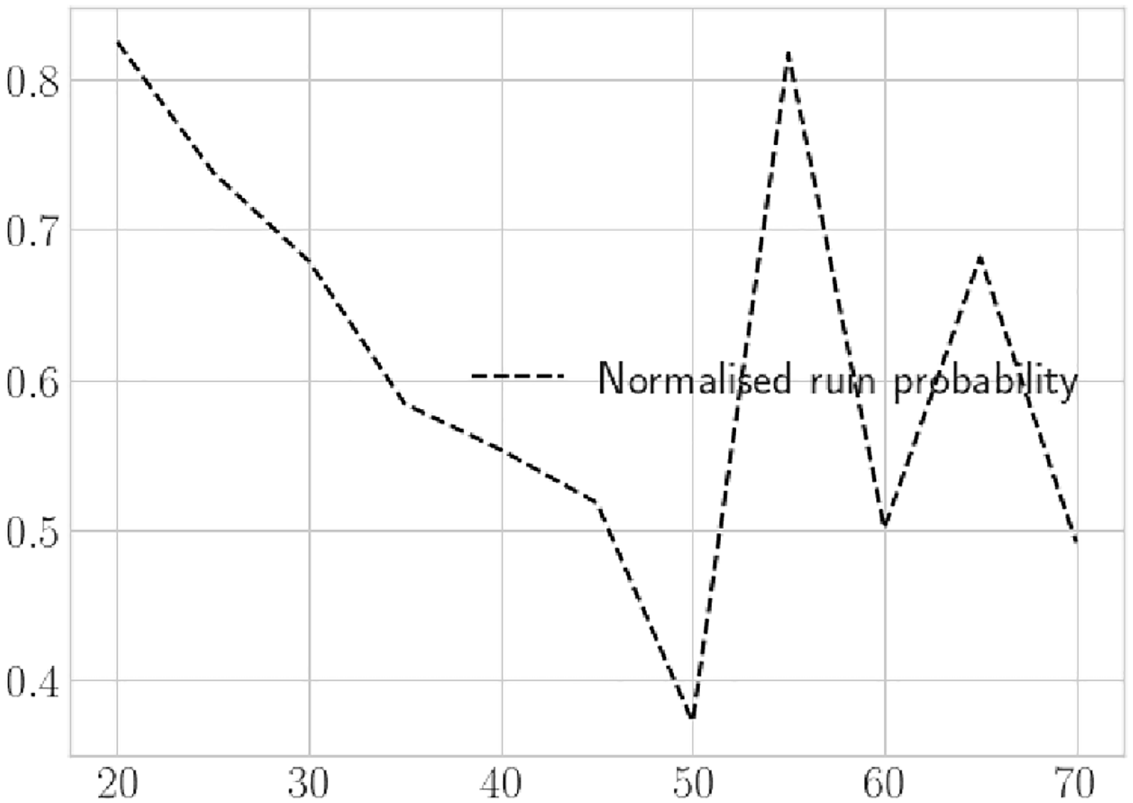
The function
 $u^{\lambda}\Psi(u)$
for
 $\lambda=0.125$
.

9. Monte Carlo simulations
In this section we present the results of the numerical analysis carried out using Monte Carlo simulations for the model (2.4) with
 $\mathbf{a}(x)=(\lambda+1)\sigma^{2}(x)/2$
and
 $\sigma\equiv 0.1$
, in which
 $\xi_{k}$
are i.i.d. Gaussian (0,1) RVs and
 $(N_{t})_{t\ge 0}$
is the homogeneous Poisson process with the intensity
 $1.5$
. To calculate the ruin probability (2.7), 100 independent Monte Carlo simulations were performed. In Table 1 we show the behavior of the ruin probability
 $\Psi(u)$
and the normalized ruin probability
 $u^{\lambda}\Psi(u)$
as functions of the initial capital
 $u>0$
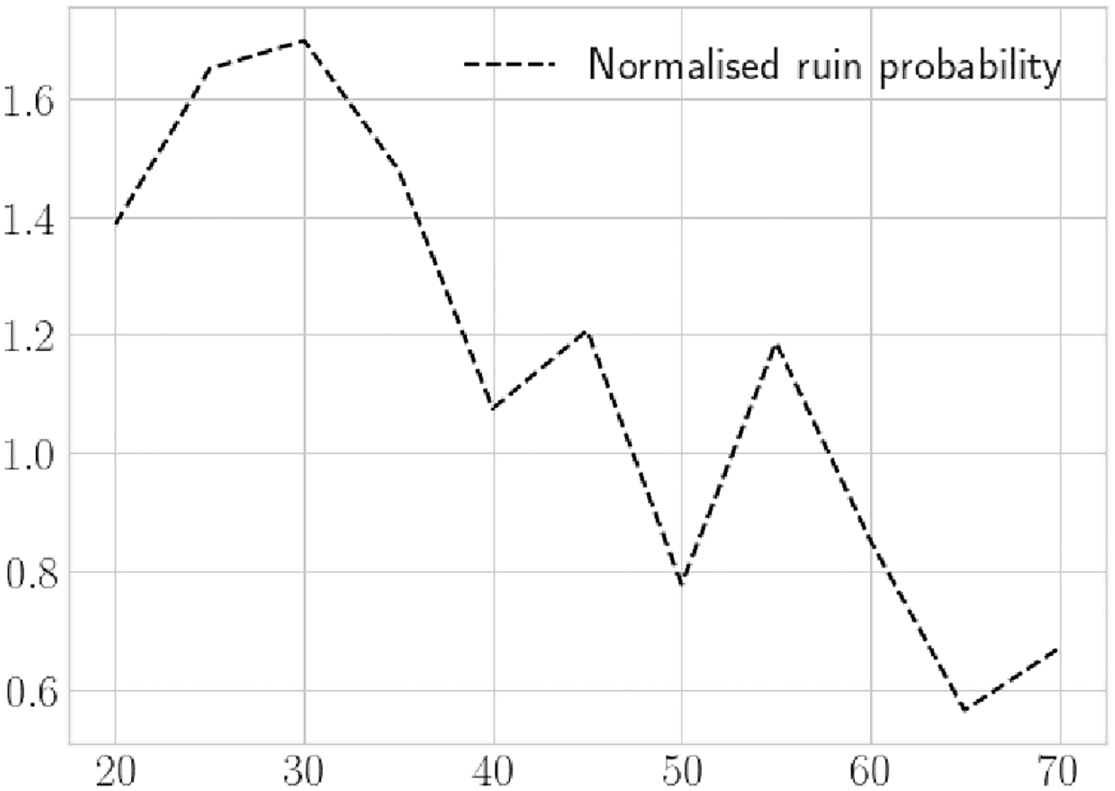
. Moreover, in Figures 1–3 these behaviors are illustrated graphically, where the abscissa axis presents the initial capitals and the ordinate axis gives the values of the normalized ruin probability
 $u^{\lambda}\Psi(u)$
. As we can see, the Monte Carlo simulations completely confirm the theoretical results obtained in Theorem 4.4, i.e. the normalized probability is always bounded.
The function
 $u^{\lambda}\Psi(u)$
for
 $\lambda=0.25$
.
10. Conclusion
In conclusion, we highlight the main results and their significance.
-
• First of all, it should be emphasized that the results obtained are of great importance for applied probability theory, and especially for the Markov renewal theory developed in [Reference Kesten14, Reference Klüppelberg and Pergamenchtchikov15]. Indeed, this paper considers the ruin problem for the model (2.4) that cannot be studied using the traditional actuarial mathematics methods, and only the Markov renewal theory (Theorem 6.1) can provide the necessary asymptotic properties for the ruin probabilities.
-
• Furthermore, probably for the first time the ruin problem for the Sparre–Andersen model with investments in the stochastic volatility model (2.2) is studied completely. The conditions under which the ruin probability goes to zero are found. The obtained convergence rate is given by the power function, i.e.
 $u^{-\lambda}$
, where the exponent
$\lambda>0$
is the root of equation (3.3) and is independent of the initial values of the Markov chain
$(\theta_{t})_{t\ge 0}$
.
-
• Moreover, in Remark 4.3 we construct the financial strategy for which this root is found in the explicit form. The practical significance of these results is that for any sufficiently small
$0 < {\delta} < 1$
the constructed investment strategy provides the decay of the ruin probability with power rate
$u^{{1-2} / {\delta}}$
, which is more rapid than any power function. It should be noted that no conditions for the model (1.1) are assumed, even the classical ‘net profit’ condition as in the Cramér–Lundberg model. This means that if in the framework of the Cramér–Lundberg model the ‘net profit’ condition does not hold, then to avoid ruin the company has to invest in risky assets a small fraction of its capital to obtain the ruin probability tending to zero with a rate more rapid than any power one. This is a surprising result for such problems. -
• Also, we note that the company should invest only in markets for which condition (2.9) is met. This property of the market allows companies not to lose money in the absence of a net profit condition, since in this case risky assets are income-producing. In Remark 4.3 we explain how this condition can be obtained for any markets (2.2) with positive returns
$a_{0,t}>0$
.


The function
 $u^{\lambda}\Psi(u)$
for
 $\lambda=0.5$
.
Appendix A. Proofs of auxiliary results
A.1. Proof of Proposition 3.3
Proof. Assume that the random variables
 $(\tau_{j})_{j\ge 1}$
in (1.2) are exponential with parameter
 $q>\sigma^{2}_{\mathrm{max}}\rho_{\mathrm{max}}(\rho_{\mathrm{max}}-\rho_{*})/2$
. Note that, for any
 $\lambda>0$
,
 \begin{align*} {\mathbb E}_{x} A^{\lambda}_{1} &= {\mathbb E}_{x}\exp\bigg\{ \int^{\mathbf{t}_{1}}_{0} g_{\lambda}(\theta_{s})\,\mathrm{d} s\bigg\} = q {\mathbb E}_{x} \int^{\infty}_{0}\exp\bigg\{\int^{t}_{0} g_{\lambda}(\theta_{s})\,\mathrm{d} s-qt\bigg\}\, \mathrm{d} t, \\[3pt] g_{\lambda}(x) &= \frac{\lambda}{2} \sigma^{2}(x) (\lambda-\rho(x)). \end{align*}
Therefore,
 $0 < \min_{x\in\mathcal{X}}g_{\lambda}(x) \le \max_{x\in\mathcal{X}}g_{\lambda}(x) < q$
for any
 \begin{align*} \rho_{\mathrm{max}}<\lambda<\frac{\rho_{*}}{2} +\sqrt{\frac{8q+\sigma^{2}_{\mathrm{max}}\rho^{2}_{*}}{4\sigma^{2}_{\mathrm{max}}}}, \end{align*}
which means that for such
 $\lambda$
we get
 $1< \min_{x\in\mathcal{X}}{\mathbb E}_{x} A^{\lambda}_{1} \le \max_{x\in\mathcal{X}}{\mathbb E}_{x} A^{\lambda}_{1} <\infty$
. Hence, Proposition 3.3.
A.2. Proof of Proposition 7.1
Proof. First, note that in view of (2.12) we can rewrite the RVs
 $\mathbf{u}_{j}$
as
 \begin{align*} \mathbf{u}_{j} = - \int^{\mathbf{t}_{j}}_{\mathbf{t}_{j-1}}\widetilde{\mathbf{a}}(\theta_{s})\, \mathrm{d} s - \int^{\mathbf{t}_{j}}_{\mathbf{t}_{j-1}} \sigma(\theta_{s})\, \mathrm{d} W_{s} =- \int^{\tau_{j}}_{0} \widetilde{\mathbf{a}}_{j}(s)\, \mathrm{d} s - \int^{\tau_{j}}_{0} \sigma_{j}(s)\, \mathrm{d} W^{j}_{s}, \end{align*}
where
 $\widetilde{\mathbf{a}}_{j}(s)=\widetilde{\mathbf{a}}(\theta_{ \mathbf{t}_{j-1}+s})$
,
 $\sigma_{j}(s)=\sigma(\theta_{\mathbf{t}_{j-1}+s})$
, and
 $W^{j}_{s}=W^{j}_{s+\mathbf{t}_{j-1}}-W^{j}_{\mathbf{t}_{j-1}}$
. It is clear that
 $(W^{j})_{j\ge 1}$
are independent Wiener processes. Therefore, the RVs
 $(\mathbf{u}_{j})_{j\ge 1}$
are conditionally independent with respect to
 $\sigma\{(\theta_{t},N_{t})_{t\ge 0}\}$
. Let
 $\beta_{n}=f(z_{n+1},\ldots,z_{n+m})$
; we need to show that
 \begin{equation} {\mathbb E}(\beta_{n}\mid\mathcal{F}_{n}) = \overline{f}(x_{n}), \end{equation}
where
 $\overline{f}(x)={\mathbb E}_{x}\beta_{0}$
. Indeed, let
 $\zeta_{n}$
be a bounded
 $\mathcal{F}_{n}$
-measurable RV. Then
 \begin{align*} {\mathbb E}\,\zeta_{n}\beta_{n} = \int_{{\mathbb R}^{n+m}} \int_{\mathcal{B}^{n+m}} {\mathbb E}^{\theta}\zeta_{n}\beta_{n} \prod^{n+m}_{j=1} \prod^{n+m}_{j=1} \eta(\mathrm{d} s_{j})\, \mu_{\mathrm{W}}(\mathrm{d} y_{j}), \end{align*}
where
 $\mathcal{B}=\mathcal{C}[0,+\infty)$
is the Banach space of continuous
 $[0,+\infty)\to{\mathbb R}$
functions,
 $\mu_{\mathrm{W}}$
is the Wiener measure in
 $\mathcal{B}$
,
 ${\mathbb E}^{\theta}$
is the expectation under the condition that
 $\tau_{j}=s_{j}$
, and
 $W^{j}(s)=y_{j}(s)$
for all
 $s\ge 0$
. Then
 ${\mathbb E}^{\theta}\zeta_{n}\beta_{n}= {\mathbb E}^{\theta}\zeta_{n} {\mathbb E}^{\theta}\big( \beta_{n} \mid \mathcal{G}^{\theta}_{\mathbf{t}_{n}} \big)$
,
 $\mathcal{G}^{\theta}_{t}=\sigma\{\theta_{u}, 0\le u\le t\}$
, and
 $\mathbf{t}_{n}=\sum^{n}_{i=1}s_{i}$
. Note that in this case
 ${\mathbb E}^{\theta}\big( \beta_{n} \mid \mathcal{G}^{\theta}_{\mathbf{t}_{n}} \big)= \check{\beta}\big(\theta_{t_{n}}\big)$
and
 $\check{\beta}(x)= {\mathbb E}^{\theta}_{x}\,f\big(\check{z}^{(n)}_{1},\ldots,\check{z}^{(n)}_{m}\big)$
, where
 $\check{z}^{(n)}_{j}=(\theta_{\check{\mathbf{t}}_{j}},\check{\mathbf{u}}_{j})$
,
 $\check{\mathbf{t}}_{j}=\sum^{n+j}_{i=n+1}s_{i}$
, and
 $\check{\mathbf{u}}_{j}= - \int^{s_{n+j}}_{0} \check{\mathbf{a}}_{j}(v)\, \mathrm{d} v - \int^{s_{n+j}}_{0} \check{\sigma}_{j}(v)\, \mathrm{d} y_{j}(v)$
with
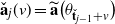 $\check{\mathbf{a}}_{j}(v)= \widetilde{\mathbf{a}}\big(\theta_{\check{\mathbf{t}}_{j-1}+v}\big)$
,
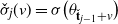 $\check{\sigma}_{j}(v)=\sigma\big(\theta_{\check{\mathbf{t}}_{j-1}+v}\big)$
and
 $\check{\mathbf{t}}_{0}=0$
. Therefore, by Fubini’s theorem we obtain that
 \begin{align}\nonumber {\mathbb E}\,\zeta_{n}\beta_{n} &= {\mathbb E}^{\theta} \int_{{\mathbb R}^{n+m} } \int_{\mathcal{B}^{n+m}} \zeta_{n} \check{\beta}\big(\theta_{t_{n}}\big) \prod^{n+m}_{j=1} \prod^{n+m}_{j=1} \eta(\mathrm{d} s_{j})\, \mu_{\mathrm{W}}(\mathrm{d} y_{j}) \\[2mm] &= {\mathbb E}^{\theta} \int_{{\mathbb R}^{n}} \int_{\mathcal{B}^{n}} \zeta_{n} \overline{\beta}\big(\theta_{\mathbf{t}_{n}}\big) \prod^{n}_{j=1} \prod^{n}_{j=1} \eta(\mathrm{d} s_{j})\, \mu_{\mathrm{W}}(\mathrm{d} y_{j}) = {\mathbb E}\, \zeta_{n} \overline{\beta}\big(\theta_{\mathbf{t}_{n}}\big), \end{align}
where
 \begin{equation*} \overline{\beta}(x)= \int_{{\mathbb R}^{m}} \int_{\mathcal{B}^{m}} \check{\beta}(x) \prod^{n+m}_{j=n+1} \prod^{n+m}_{j=n+1} \eta(\mathrm{d} s_{j})\, \mu_{\mathrm{W}}(\mathrm{d} y_{j}) =\int_{{\mathbb R}^{m}} \int_{\mathcal{B}^{m}} \check{\beta}(x) \prod^{m}_{j=1} \prod^{m}_{j=1} \eta(\mathrm{d} s_{j})\, \mu_{\mathrm{W}}(\mathrm{d} y_{j}). \end{equation*}
In this case, using again Fubini’s theorem we find that
 \begin{equation*} \overline{\beta}(x) = {\mathbb E}^{\theta}_{x} \int_{{\mathbb R}^{m}} \int_{\mathcal{B}^{m}} f\big(\check{z}^{(n)}_{1},\ldots,\check{z}^{(n)}_{m}\big) \prod^{m}_{j=1} \prod^{m}_{j=1} \eta(\mathrm{d} s_{j})\, \mu_{\mathrm{W}}(\mathrm{d} y_{j}) = {\mathbb E}_{x} f(z_{1},\ldots,z_{m}) =\overline{f}(x). \end{equation*}
Now the equality (A.2) implies that
 ${\mathbb E}(\beta_{n}\mid\mathcal{F}_{n})=\overline{f}\big(\theta_{\mathbf{t}_{n}}\big)=\overline{f}(x_{n})$
, i.e. we obtain (A.1), which is the first equality in Proposition 7.1. Moreover, we can check directly that, for any bounded measurable
 $\mathcal{Z}^{m}\to{\mathbb R}$
function f,
 \begin{align*} \widetilde{{\mathbb E}}\big(\,f(z_{n+1},\ldots,z_{n+m}) \mid \mathcal{F}_{n}\big) =\frac{1}{h(x_{n})} {\mathbb E}\big(\,f_{1}(z_{n+1},\ldots,z_{n+m}) \mid \mathcal{F}_{n}\big), \end{align*}
where
 $f_{1}(z_{n+1},\ldots,z_{n+m}) =\prod^{m}_{j=1}{\mathrm{e}}^{\lambda \mathbf{u}_{n+j}} h(x_{n+m}) f(z_{n+1},\ldots, z_{n+m})$
. Therefore, the equality (A.1) implies this proposition.
A.3. Proof of Lemma 3.1
Proof. First, we note that the definition in (2.12) implies that
 \begin{align*} {\mathbb E}_{x} A^{\delta}_{1} = {\mathbb E}_{x}\exp\bigg\{\frac{\delta}{2}\int^{\mathbf{t}_{1}}_{0} \sigma^{2}(\theta_{v}) (\delta-\varrho(\theta_{v}))\,\mathrm{d} v\bigg\}, \qquad \varrho(x) = \frac{2\mathbf{a}(x)}{ \sigma^2(x)}-1. \end{align*}
Using the condition (2.9) and choosing
 $0 < \delta < \rho_{*}$
, we get
 \begin{align*} \mathbf{r}= \max_{x\in\mathcal{X}}\, {\mathbb E}_{x}\,A^{\delta}_{1} \le {\mathbb E}\,{\mathrm{e}}^{-\delta_{1}\tau_{1}} =\int^{+\infty}_{0} {\mathrm{e}}^{-\delta_{1} x}\,\eta(\mathrm{d} x) <1, \end{align*}
where
 $\delta_{1}=\delta(\rho_{*}-\delta)\sigma_{*}/2$
. Furthermore, for any
 $n\ge 2$
, through Proposition 7.1 we obtain that, for any
 $x\in\mathcal{X}$
,
 ${\mathbb E}_{x} \prod^{n}_{j=1} A^{\delta}_{j} = {\mathbb E}_{x} \prod^{n-1}_{j=1} {\mathrm{e}}^{\delta\mathbf{u}_{j}} {\mathbb E} \big({\mathrm{e}}^{\delta\mathbf{u}_{n}} \mid \mathcal{F}_{n-1}\big) ={\mathbb E}_{x} \prod^{n-1}_{j=1} {\mathrm{e}}^{\delta\mathbf{u}_{j}} H(x_{ n-1})$
, where
 $H(x)={\mathbb E}_{x}\,{\mathrm{e}}^{\delta \mathbf{u}_{1}} ={\mathbb E}_{x} A^{\delta}_{1} \le \mathbf{r}<1$
. This implies that, for any
 $n\ge 2$
,
 \begin{align*} {\mathbb E}_{x} \prod^{n}_{j=1} A^{\delta}_{j} \le \mathbf{r} {\mathbb E}_{x} \prod^{n-1}_{j=1} A^{\delta}_{j} \end{align*}
and, therefore, by induction we deduce that
 \begin{equation} \sup\nolimits_{x\in\mathcal{X}} {\mathbb E}_{x} \prod^{n}_{j=1} A^{\delta}_{j} \le \mathbf{r}^{n}. \end{equation}
Therefore,
 ${\mathbb E} \big( \sum_{n\ge 1}\, |\xi_{n}| {\mathbb E}\prod^{n}_{j=1} A_{j} \big)^{\delta} \le {\mathbb E}|\xi_{1}|^{\delta} \sum_{n\ge 1}\,{\mathbb E}\prod^{n}_{j=1} A^{\delta}_{j} \le {\mathbb E}|\xi_{1}|^{\delta} \sum_{n\ge 1}\,\mathbf{r}^{n} <\infty$
, i.e.
 $\sum_{n\ge 1} |\xi_{n}| \prod^{n}_{j=1} A_{j} <\infty$
a.s. and we obtain the convergence (3.1).
A.4. Geometric ergodicity property of the chain
$(\textbf{\textit{x}}_{\textbf{\textit{n}}})_{\textbf{\textit{n}} \ge 0}$

Proof. In this section we show Lemma 3.2. To this end, we note that in view of Condition 3.2 there exists
 $\kappa_{*}\in\mathcal{X}$
for which
 $\mathbf{p}_{*}=\min_{x\neq \kappa_{*}}{\mathbb P}_{x}(x_{1}= \kappa_{*})>0$
. Moreover, we choose the
 $\mathcal{X}\to [1,\infty)$
Lyapunov function V as
 $V(x)=1+\mathbf{l}_{*}\mathbf{1}_{\{x\neq \kappa_{*}\}}$
, where the parameter
 $\mathbf{l}_{*}>0$
will be specified later. Then in this case, for
 $x\neq \kappa_{*}$
,
 \begin{align*} {\mathbb E}_{x}\,V(x_{1}) &= \sum_{z\in\mathcal{X}}\,V(z) {\mathbb P}_{x}(x_{1}=z) = {\mathbb P}_{x}(x_{1}= \kappa_{*}) + \sum_{z\neq \kappa_{*}}\,V(z) {\mathbb P}_{x}(x_{1}=z) \\[3pt] &= \bigg( \frac{{\mathbb P}_{x}(x_{1}=x_{*})}{1+\mathbf{l}_{*}} + {\mathbb P}_{x}(x_{1}\neq \kappa_{*}) \bigg) V(x)\\[3pt] &= \bigg( \frac{{\mathbb P}_{x}(x_{1}=x_{*})}{1+\mathbf{l}_{*}} + 1-{\mathbb P}_{x}(x_{1}=\kappa_{*}) \bigg) V(x) \le \varrho^{*} V(x), \end{align*}
where, in view of choosing the point
 $\kappa_{*}$
for sufficiently large
 $\mathbf{l}_{*}>0$
,
 \begin{align*} \varrho^{*}= \frac{1}{1+\mathbf{l}_{*}} + 1-\mathbf{p}_{*} <1. \end{align*}
This means that, for any
 $x\in\mathcal{X}$
,
 ${\mathbb E}_{x}\,V(x_{1})\le \varrho^{*}\, V(x) +(1+\mathbf{l}_{*}) \mathbf{1}_{\{x=\kappa_{*}\}}$
, i.e. the drift condition [Reference Meyn and Tweedie17, (V4)] holds for the set
 $C=\{\kappa_{*}\}$
. Therefore, in view of [Reference Meyn and Tweedie17, Theorem 15.0.1], we obtain this lemma.
A.5. Property of the distribution (7.4)
Lemma A.1 There exists a number
 $\rho>0$
such that, for any
 $x\in\mathcal{X}$
,
 \begin{equation} \lim_{n\to\infty} \widetilde{{\mathbb P}}_{x} \big( \Pi_{n} < {\mathrm{e}}^{\rho n} \big) =0, \end{equation}
where
 $\Pi_{n}=\prod^{n}_{j=1} A_{j}$
.
Proof. First, we set
 $\Gamma_{n}=\{\Pi_{n}<{\mathrm{e}}^{\rho n}\}$
. From the definition in (7.4) it follows that
 \begin{align*} \widetilde{{\mathbb P}}_{x}\big(\Gamma_{n}) = \frac{1}{h(x)} {\mathbb E}_{x} \Pi^{\lambda}_{n}\,h(x_{n}) \mathbf{1}_{\Gamma_{n}} \le \frac{h^{*}}{h(x)} {\mathbb E}_{x} \Pi^{\lambda}_{n} \mathbf{1}_{\Gamma_{n}}, \end{align*}
where
 $h^{*}=\max_{x\in\mathcal{X}}h(x)$
. Therefore, using the bound in (A.3), we obtain that, for any
 $\epsilon>0$
,
 \begin{align*} \widetilde{{\mathbb P}}_{x}(\Gamma_{n}) \le \frac{h^{*}}{h(x)} \big( \epsilon^{\lambda} + {\mathrm{e}}^{\rho n} {\mathbb P}_{x}(\Pi_{n} >\epsilon) \big ) \le \frac{h^{*}}{h(x)} \big ( \epsilon^{\lambda} + \epsilon^{-\delta} \mathbf{r}^{n} {\mathrm{e}}^{\rho n} \big ). \end{align*}
Choosing
 $0 < \rho < -\ln \mathbf{r}$
, we get the limit (A.4). Hence Lemma A.1.
A.6. Property of the RV R
Proof. First, we show the equality (7.5). To do this we note that Lemma 3.1 implies directly that
 $R_{1}=\lim_{m\to\infty} R_{1,m}$
a.s., where
 $R_{1,m}=\sum^{m}_{k= 2} \xi_{k} \prod_{j=2}^{k} A_{j} = \sum^{m}_{k= 2} \xi_{k} \prod_{j=2}^{k} {\mathrm{e}}^{\mathbf{u}_{j}}$
. Now let f be a bounded continuous
 ${\mathbb R}_{+}\to{\mathbb R}$
function. Then, through the dominated convergence theorem,
 ${\mathbb E}(\,f(R_{1})\mid\mathcal{F}_{1})= \lim_{m\to\infty} {\mathbb E}(\,f(R_{1,m})\mid\mathcal{F}_{1})$
. Now, using Proposition 7.1, we obtain that, for any
 $m\ge 1$
, the expectation
 ${\mathbb E}(\,f(R_{1,m})\mid\mathcal{F}_{1})= \overline{f}(x_{1})$
, where in this case
 \begin{align*} \overline{f}(x) = {\mathbb E}_{x}\, f\Bigg( \sum^{m-1}_{k= 1} \xi_{k} \prod_{j=1}^{k} {\mathrm{e}}^{\mathbf{u}_{j}} \Bigg). \end{align*}
Again using the dominated convergence theorem, we get
 ${\mathbb E}(\,f(R_{1})\mid\mathcal{F}_{1}) = H(x_{1})$
and
 \begin{align*} H(x)= \lim_{m\to\infty} {\mathbb E}_{x}\, f\Bigg(\sum^{m-1}_{k= 1} \xi_{k} \prod_{j=1}^{k} {\mathrm{e}}^{\mathbf{u}_{j}} \Bigg) = {\mathbb E}_{x}\, f\Bigg( \lim_{m\to\infty} \sum^{m-1}_{k= 1} \xi_{k} \prod_{j=1}^{k} {\mathrm{e}}^{\mathbf{u}_{j}} \Bigg) = {\mathbb E}_{x}\, f(R). \end{align*}
Therefore,
 ${\mathbb E}(\,f(R_{1}) \mid x_{1}=x) = {\mathbb E}( {\mathbb E}(\,f(R_{1})\mid\mathcal{F}_{1}) \mid x_{1}=x ) = {\mathbb E}( H(x_{1}) \mid x_{1}=x ) = {\mathbb E}_{x}\, f(R)$
. Hence the equality (7.5).
Lemma A.2.
 $\sup\nolimits_{x\in\mathcal{X}} {\mathbb E}_{x}\, R^{q}<\infty$
for any
 $0 < q < \lambda$
.
Proof. First, note that, for any
 $x\in\mathcal{X}$
,
 \begin{align*} {\mathbb E}_{x}\, R^{q} \le\frac{\sum_{z\in\mathcal{X}}\pi(z){\mathbb E}_{z}\,R^{q}}{\pi(x)} =\frac{{\mathbb E}\,R^{q}}{\pi(x)} \le \frac{{\mathbb E}\,R^{q}}{\pi_{*}}, \end{align*}
where
 $\pi_{*}=\min_{z\in\mathcal{X}}\pi(z)$
. Proposition 3.2 implies that
 $\varkappa(q)<1$
, i.e. for some
 $\varkappa(q)<\mathbf{r}<1$
. In view of Proposition 3.1, for sufficiently large k the expectation
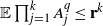 ${\mathbb E} \prod^{k}_{j=1} A^{q}_{j} \le \mathbf{r}^{k}$
. Therefore, for
 $q\le 1$
, the expectation
 ${\mathbb E}\, R^{q} \le {\mathbb E}\,|\xi_{1}|^{q} \sum_{k\ge 1} {\mathbb E} \prod^{k}_{j=1} A^{q}_{j} <\infty$
. For
 $q>1$
and some
 $\epsilon>0$
we obtain, through the Hölder inequality, that
 $R^{q}\le \mathbf{U}_{q} \sum_{k\ge 1} (1+\epsilon)^{q k} |\xi_{k}|^{q} \prod^{k}_{j=1} A^{q}_{j}$
, where
 $\mathbf{U}_{q}=((1+\epsilon)^{q/(q-1)}-1)^{1-q}$
. From this, it follows that, for any
 $0 < \epsilon < \mathbf{r}^{-1/q}-1$
, the expectation
 ${\mathbb E}\, R^{q} \le {\mathbb E}\,|\xi_{1}|^{q} \mathbf{U}_{q} \sum_{k\ge 1} (1+\epsilon)^{q k} {\mathbb E} \prod^{k}_{j=1} A^{q}_{j} <\infty$
. Hence Lemma A.2.
A.7. Komlos’ theorem
Now we need the following well-known Komlos result (see, for example, [Reference Kabanov and Pergamenshchikov10, Section A7]).
Theorem A.1. Assume that
 $(\xi_{n})_{n\ge 1}$
is a sequence of integrable RVs with
 $\sup\nolimits_{n\ge 1}{\mathbb E}\,|\xi_{n}| <\infty$
. Then there exists a subsequence
 $(\xi_{n_{k}})_{k\ge 1}$
and an RV
 $\zeta$
with
 ${\mathbb E}\,|\zeta|<\infty$
such that
 \begin{align*} \lim_{k\to\infty} \frac{\xi_{n_{1}}+\cdots+\xi_{n_{k}}}{k} =\zeta \quad \textit{a.s.} \end{align*}
A.8. Proof of the representation (7.7)
Proof. Let
 $\mathbf{B}(\mathcal{X},{\mathbb R})$
be the linear space of bounded, measurable,
 $\mathcal{X}\times{\mathbb R}\to{\mathbb R}$
functions, and
 $\mathbf{L}$
be a linear renewal
 $\mathbf{B}(\mathcal{X},{\mathbb R})\to \mathbf{B}(\mathcal{X},{\mathbb R})$
operator defined as
 \begin{equation} \mathbf{L}(\,f)(x,t)=\widetilde{{\mathbb E}}_{x}\,f(x_{1},t-\mathbf{u}_{1}). \end{equation}
Using this definition in (7.6), the function
 $\widetilde{Z}(x,t)$
can be represented in the form
 \begin{equation} \widetilde{Z}(x,t)= \mathbf{L}(\widetilde{Z})(x,t) + \widetilde{g}(x,t). \end{equation}
Now we need to calculate the nth power for the operator defined in (A.5). Let us show that, for any
 $m\ge 1$
and any
 $\mathcal{X}\times{\mathbb R}\to{\mathbb R}$
functions,
 \begin{equation} \mathbf{L}^{m}(h)(x,t)=\widetilde{{\mathbb E}}_{x}\,h(x_{m},t-\mathbf{s}_{m}), \end{equation}
where
 $\mathbf{s}_{m}=\sum^{m}_{j=1}\mathbf{u}_{j}$
. To do this we use the induction method. Indeed, for
 $m=1$
this is true due to the definition (A.5). Assume now that this holds for m. Then the
 $(m+1)$
th power can be calculated as
 $\mathbf{L}^{m+1}(h)(x,t)=L(\check{h})(x,t)= \widetilde{{\mathbb E}}_{x}\, \check{h}(x_{1},t-\mathbf{u}_{1})$
, where
 $\check{h}(x,t)=\mathbf{L}^{m}(h)(x,t)= \widetilde{{\mathbb E}}_{x}\,h(x_{m},t-\mathbf{s}_{m})$
. Note that through the property (6.1) for the distribution (7.4) we obtain that
 $\check{h}(x_{1},t-\mathbf{u}_{1})= \widetilde{{\mathbb E}}(h(x_{m+1},t-\mathbf{s}_{m+1}) \mid\mathcal{F}_{1} )$
, i.e.
 \begin{align*} \mathbf{L}^{m+1}(h)(x,t)= \widetilde{{\mathbb E}}_{x}\, \widetilde{{\mathbb E}}(h(x_{m+1},t-\mathbf{s}_{m+1}) \mid\mathcal{F}_{1} )= \widetilde{{\mathbb E}}_{x}\, h(x_{m+1},t-\mathbf{s}_{m+1}). \end{align*}
Therefore, the property (A.7) holds for any
 $m\ge 1$
. Moreover, note that, for any
 $m\ge 1$
the equality (A.6) implies the representation for the function
 $\widetilde{Z}(x,t)$
 \begin{equation} \widetilde{Z}(x,t) = \mathbf{L}^{m}(\widetilde{Z})(x,t) + \sum^{m-1}_{j=0} \mathbf{L}^{j}(\widetilde{g})(x,t). \end{equation}
From (A.7) it now follows that
 \begin{equation*} \mathbf{L}^{m}(\widetilde{Z})(x,t)= \frac{1}{h(x)} {\mathbb E}_{x}\prod^{m}_{j=1} A^{\lambda}_{j} Z(x_{m},t-\mathbf{s}_{m}) = \frac{1}{h(x)} {\mathbb E}_{x} \prod^{m}_{j=1} A^{\lambda}_{j} {\mathrm{e}}^{-(t-\mathbf{s}_{m})} \int^{t-\mathbf{s}_{m}}_{0} v^{\lambda} \Upsilon(x_{m},v)\, \mathrm{d} v, \end{equation*}
where
 $\Upsilon(x,v)={\mathbb P}_{x}(R>v)$
. Using the condition (6.1), we can represent the last term as
 $\Upsilon(x_{m},v) ={\mathbb E}\big(\mathbf{1}_{\{R_{m}>v\}}\mid\mathcal{F}_{m}\big)$
, where
 \begin{align*} R_{m}= \sum^{\infty}_{k=m+1} \xi_{k} \prod^{k}_{j=m+1} A_{j} = \sum^{\infty}_{n=1} \xi_{n+m} \prod^{n+m}_{j=m+1} A_{j} = \sum^{\infty}_{n=1} \xi_{n+m} \prod^{m}_{l=1} {\mathrm{e}}^{u_{m+l}}. \end{align*}
Therefore,
 \begin{align*} \mathbf{L}^{m}(\widetilde{Z})(x,t) &= \frac{1}{h(x)} {\mathbb E}_{x} \prod^{m}_{j=1} A^{\lambda}_{j} {\mathrm{e}}^{-(t-\mathbf{s}_{m})} \int^{t-\mathbf{s}_{m}}_{0} v^{\lambda} \mathbf{1}_{\{R_{m}>v\}}\, \mathrm{d} v\\[3pt] &= \frac{1}{{\mathrm{e}}^{t}h(x)} \int^{t}_{0} y^{\lambda} {\mathbb P}_{x}\Bigg( \prod^{m}_{j=1} A_{j} R_{m}>y\Bigg)\, \mathrm{d} y. \end{align*}
Through Chebyshev’s inequality we obtain that, for any
 $y>0$
and for sufficiently small
 $\delta>0$
,
 \begin{align*} {\mathbb P}_{x}\Bigg( \prod^{m}_{j=1} A_{j} R_{m}>y\Bigg) \le \frac{1}{y^{\delta}} {\mathbb E}_{x} \prod^{m}_{j=1} A^{\delta}_{j} R^{\delta}_{m} = \frac{1}{y^{\delta}} {\mathbb E}_{x} \prod^{m}_{j=1} A^{\delta}_{j} {\mathbb E}\big(R^{\delta}_{m}\mid\mathcal{F}_{m}\big). \end{align*}
Using again the condition (6.1) and Lemma A.2, which holds for sufficiently small
 $\delta>0$
, we obtain that
 ${\mathbb E}\big(R^{\delta}_{m}\mid\mathcal{F}_{m}\big) = {\mathbb E}_{x_{m}}R^{\delta} \le \sup_{z\in\mathcal{X}} {\mathbb E}_{z}R^{\delta} <\infty$
. Therefore, the bound in (A.3) with a small
 $\delta>0$
implies directly that, for some constants
 $c>0$
and
 $0 < \mathbf{r} < 1$
,
 \begin{align*} {\mathbb P}_{x}\Bigg( \prod^{m}_{j=1} A_{j} R_{m}>y\Bigg) \le \frac{c}{y^{\delta}} \mathbf{r}^{m}, \end{align*}
i.e.
 $\lim_{m\to\infty} \mathbf{L}^{m}(\widetilde{Z})(x,t)=0$
. So, taking
 $m\to\infty$
in (A.8), we obtain (7.7).
A.9. A property of the function
$\textbf{\textit{g}}_{0}$

Lemma A.3. Under Condition 3.4 the function
 $g_{0}(x,t)$
defined in (7.3) is positive for any
 $x\in\mathcal{X}$
and
 $t>0$
.
Proof. In view of Condition 3.4, the density
 $\mathbf{p}_{\xi}$
of the variables
 $(\xi_{k})_{k\ge 1}$
is symmetric and non-increasing on
 ${\mathbb R}_{+}$
; then the function
 $g_{0}$
can be represented as
 \begin{align*} g_{0}(x,t) = {\mathbb P}_{x}( R>t) - {\mathbb P}_{x}( A_{1} R_{1}>t) =\int^{\infty}_{0} \delta_{t}(x,v) \mathbf{p}_{\xi}(v)\,\mathrm{d} v, \end{align*}
where
 $\delta_{t}(x,v)= {\mathbb P}_{x}(\widetilde{t}-v< R_{1}\le \widetilde{t}) - {\mathbb P}_{x}(\widetilde{t}< R_{1}\le \widetilde{t}+v)$
and
 $\widetilde{t}=t/A_{1} =t{\mathrm{e}}^{-\mathbf{u}_{1}}$
. Moreover, from Proposition 7.1 we obtain that
 $\delta_{u}(x,v)={\mathbb E}_{x}\big( \int^{\widetilde{t}}_{\widetilde{t}-v} \mathbf{q}_{x_{1}}(y)\,\mathrm{d} y -\int^{\widetilde{t}+v}_{\widetilde{t}}\mathbf{q}_{x_{1}}(y)\,\mathrm{d}y\big),$
where
 $\mathbf{q}_{x}$
is the density of the RV R under the condition that
 $\theta_{0}=x$
for
 $x\in\mathcal{X}$
. Condition 3.4 implies that the RV R also has symmetric density
 $\mathbf{q}_{x}$
which is decreasing on
 ${\mathbb R}_{+}$
. Therefore, if
 $v\le \widetilde{t}$
then, for any
 $x\in\mathcal{X}$
,
 $\int^{\widetilde{t}}_{\widetilde{t}-v}\mathbf{q}_{x}(y)\,\mathrm{d} y -\int^{\widetilde{t}+v}_{\widetilde{t}}\mathbf{q}_{x}(y)\,\mathrm{d} y\ge 0$
a.s. On the other hand, for
 $v> \widetilde{t}$
, we get
 \begin{align*} \int^{\widetilde{t}}_{\widetilde{t}-v}\mathbf{q}_{x}(y)\,\mathrm{d} y -\int^{\widetilde{t}+v}_{\widetilde{t}} \,\mathbf{q}_{x}(y)\,\mathrm{d} y &= \int^{v-\widetilde{t}}_{0}\mathbf{q}_{x}(y)\,\mathrm{d} y+ \int^{\widetilde{t}}_{0}\mathbf{q}_{x}(y)\,\mathrm{d} y \\[3pt] &\quad - \int^{2\widetilde{t}}_{\widetilde{t}}\mathbf{q}_{x}(y)\,\mathrm{d} y - \int^{\widetilde{t}+v}_{2\widetilde{t}}\mathbf{q}_{x}(y)\,\mathrm{d} y\ge 0 \quad \mbox{a.s.} \end{align*}
since
 $\mathbf{q}_{x}$
is non-increasing on
 ${\mathbb R}_{+}$
. Moreover, it is clear that there exists some non-random
 $y_{*}>0$
depending on x such that
 $\mathbf{q}_{x}(y_{*}-s)>\mathbf{q}_{x}(y_{*}+s)$
a.s. for any
 $0 < s < y_{*}$
. Now we choose
 $0 < v_{0} < y_{*}/2$
for which
 ${\mathbb P}(\xi>2v_{0})>0$
. Then
 \begin{align*} \delta_{t}(x,v) \ge {\mathbb E}_{x} \mathbf{1}_{\Gamma} \bigg( \int^{\widetilde{t}}_{\widetilde{t}-v}\mathbf{q}_{x}(y)\,\mathrm{d} y -\int^{\widetilde{t}+v}_{\widetilde{t}}\mathbf{q}_{x}(y)\,\mathrm{d} y \bigg), \end{align*}
where
 $\Gamma= \{\mathbf{t}_{1} < \mathbf{k}_{0}\}\cap \{y_{*} < \widetilde{t} < y_{*}+v_{0}\}$
and
 $\mathbf{k}_{0}=\inf\{t\ge 0\colon \theta_{t}\neq x\}$
. It should be noted here that the stopping time
 $\mathbf{k}_{0}$
is an exponential RV with intensity
 $\mathbf{l}_{0}(x)>0$
(see, for example, [Reference Andersen1]). Therefore, taking into account that
 $\mathbf{t}_{1}$
and
 $\mathbf{k}_{0}$
are independent, we obtain that
 ${\mathbb P}_{x}(\mathbf{t}_{1} < \mathbf{k}_{0})={\mathbb E}\,{\mathrm{e}}^{-\mathbf{l}_{0}(x) \mathbf{t}_{1}}$
. Note now that the set
 $\{y_{*} < \widetilde{t}_{1} < y_{*}+v_{0}\}=\{z_{1} < - \mathbf{u}_{1} < z_{2}\}$
with
 $z_{1}=\ln({y_{*}}/{t})$
and
 $z_{2}=\ln (({y_{*}+v_{0}})/{t})$
. Moreover, on the set
 $\{\mathbf{t}_{1}< \mathbf{k}_{0}\}$
the RV
 $-\mathbf{u}_{1}$
coincides with the
 $\widetilde{\mathbf{a}}(x)\mathbf{t}_{1} + \sigma(x) W_{\mathbf{t}_{1}}$
, which is conditionally Gaussian with respect to
 $\mathbf{t}_{1}$
, and therefore
 \begin{align*} {\mathbb P}_{x}(z_{1} < -\mathbf{u}_{1} < z_{2}\mid\mathbf{t}_{1})=\int^{z_{2}}_{z_{1}}\varphi_{x,\mathbf{t}_{1}}(v)\,\mathrm{d} v, \end{align*}
where
 \begin{align*} \varphi_{x,t}(v)=\frac{1}{\sqrt{2\pi t}\sigma(x)} \exp\bigg\{{-}\frac{(v-\widetilde{\mathbf{a}}(x)t)^{2}}{2\sigma^{2}(x) t}\bigg\}. \end{align*}
Thus,
 ${\mathbb P}_{x}(\Gamma)= \int^{z_{2}}_{z_{1}} {\mathbb E}\,{\mathrm{e}}^{-\mathbf{l}_{0}(x)\mathbf{t}_{1}} \varphi_{x,\mathbf{t}_{1}}(v)\,\mathrm{d} v >0$
, and we obtain that, for any
 $v_{0}<v<y_{*}$
and
 $t>0$
,
 \begin{align*} \delta_{t}(x,v)\ge {\mathbb E}_{x} \mathbf{1}_{\Gamma} \int^{\widetilde{t}}_{\widetilde{t}-v}\big(\mathbf{q}_{x}(y) - \mathbf{q}_{x}(y+v)\big)\,\mathrm{d} y \ge \int^{y_{*}}_{y_{*}-v_{0}}\big(\mathbf{q}_{x}(y) - \mathbf{q}_{x}(y+v_{0})\big)\,\mathrm{d} y \,{\mathbb P}_{x} (\Gamma) >0. \end{align*}
Hence Lemma A.3.
Funding information
This work was supported by RSF grant 24-11-00191.
Competing interests
There were no competing interests to declare which arose during the preparation or publication process of this article.

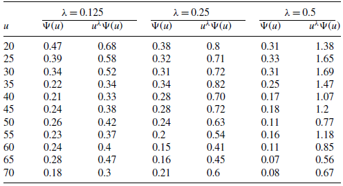
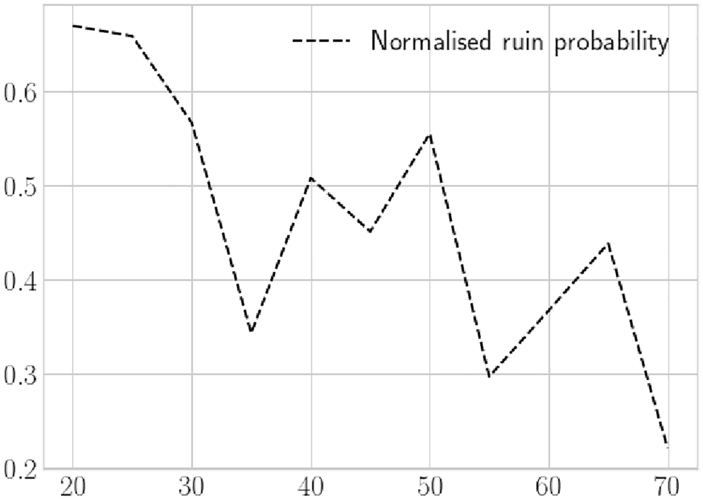
 uλΨ(u)
 λ=0.125
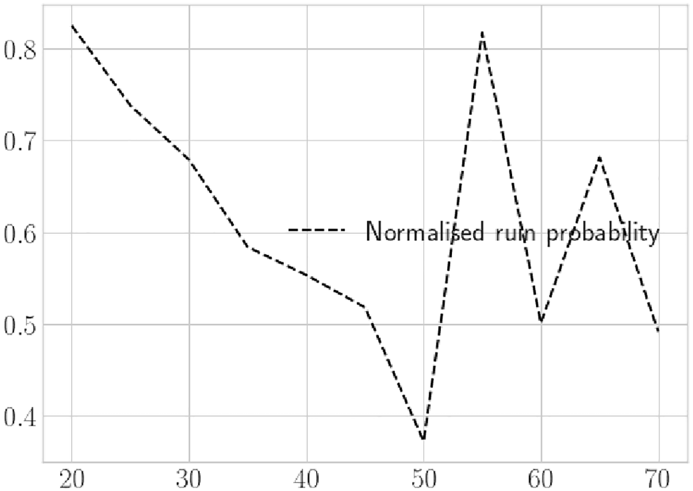
 uλΨ(u)
 λ=0.25
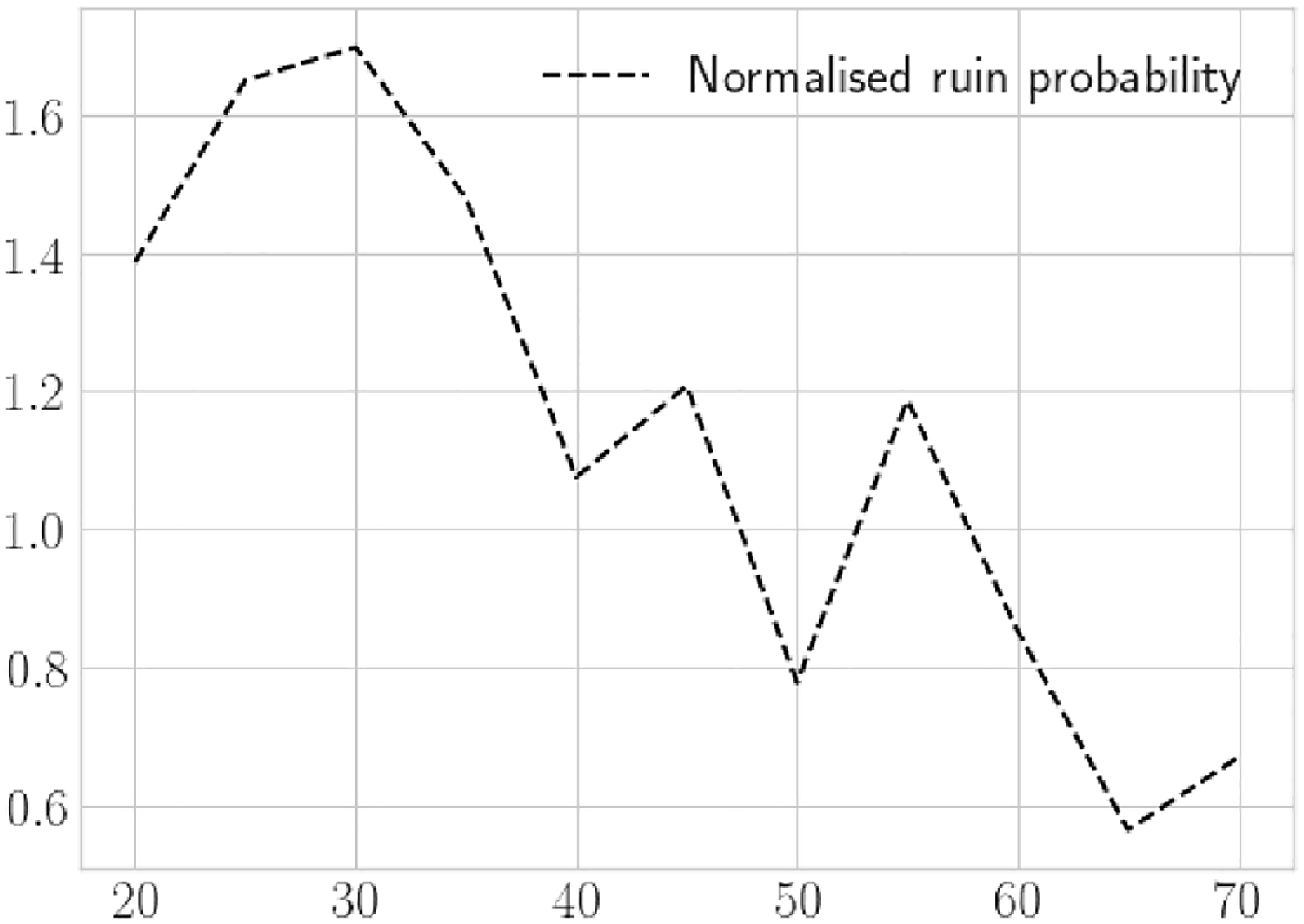
 uλΨ(u)
 λ=0.5


