1 INTRODUCTION
The risk of a financial position X is usually quantified by a law-invariant risk measure
$\xi (X)$
 , where positive values of X represent losses (e.g., negative log-returns). Two particularly desirable properties are coherence in the sense of Artzner et al. (Reference Artzner, Delbaen, Eber and Heath1999) and elicitability, which makes it possible to evaluate and compare competing point forecasts through suitable scoring functions (Gneiting, Reference Gneiting2011; Fissler and Ziegel, Reference Fissler and Ziegel2016). The ubiquitous Value-at-Risk at level
$\tau \in (0,1)$
 is the
$\tau $
 th quantile
$\mathrm {VaR}_{\tau }\equiv q_{\tau }:=\inf \{x\in \mathbb {R}:F(x)\geq \tau \}$
 of the distribution function F of the random variable X. Although intuitive, robust, and elicitable,
$\mathrm {VaR}_{\tau }$
 may fail to satisfy the subadditivity property and does not reflect the magnitude of losses beyond
$q_{\tau }$
 (Daníelsson et al., Reference Daníelsson, Embrechts, Goodhart, Keating, Muennich, Renault and Shin2001; Acerbi, Reference Acerbi2002). The notion of Expected Shortfall,
$\mathrm {ES}_{\tau }:=(1-\tau )^{-1}\int _{\tau }^{1}q_t\,\mathrm {d}t$
 , addresses these shortcomings and has become the regulatory standard for market risk under the Basel Accords III/IV (Acerbi and Tasche, Reference Acerbi and Tasche2002; Wang and Zitikis, Reference Wang and Zitikis2021); when X is continuous, it equals
$\mathbb {E}(X|X>q_{\tau })$
 (Rockafellar and Uryasev, Reference Rockafellar and Uryasev2002). Yet
$\mathrm {ES}_{\tau }$
 is not directly elicitable, but only jointly elicitable with
$\mathrm {VaR}_{\tau }$
 (Gneiting, Reference Gneiting2011; Fissler and Ziegel, Reference Fissler and Ziegel2016). This trade-off motivates the search for law-invariant risk measures that combine coherence and elicitability.
The alternative concept of expectiles has axiomatic and practical properties that strike a delicate balance between those of the two aforementioned competing risk measures. First envisioned by Aigner, Amemiya, and Poirier (Reference Aigner, Amemiya and Poirier1976) and popularized by Newey and Powell (Reference Newey and Powell1987) in a regression context, the
$\tau $
 th expectile can be defined as

Subtracting the (unimportant in practice) term
$| \tau -\mathbb {1}\{ X\leq 0 \} | X^2$
 in the cost function ensures that
$\xi _{\tau }$
 exists as the unique minimizer in the above optimization problem as soon as
$\mathbb {E}|X|<\infty $
 . Expectiles factor in both the probability and magnitude of tail realizations (Kuan, Yeh, and Hsu, Reference Kuan, Yeh and Hsu2009). While the measure is categorized alongside quantiles into the same class of M-quantiles defined by Breckling and Chambers (Reference Breckling and Chambers1988), it distinguishes itself within this class by being the only M-quantile that satisfies the coherence property (Bellini et al., Reference Bellini, Klar, Müller and Gianin2014). In fact, expectiles are the only coherent and law-invariant risk measure that is also elicitable, as shown by Ziegel (Reference Ziegel2016). They also enjoy intuitive financial interpretations in the form of their acceptance sets and their connection to the gain-loss ratio (Bellini and Di Bernardino, Reference Bellini and Di Bernardino2017). A proper comparison between expectiles and quantiles when they are identical for different
$\tau $
 levels, thus defining a market risk measure with the same meaning and properties, is provided by Daouia, Girard, and Stupfler (Reference Daouia, Girard and Stupfler2018) from an extreme value perspective. Philipps (Reference Philipps2022) has developed a range of further interpretations of expectiles from multiple analytical perspectives. Although not comonotonically additive, that is,
$\xi _{\tau }(X+Y)\neq \xi _{\tau }(X)+\xi _{\tau }(Y)$
 for comonotonic random variables X and Y (Acerbi and Székely, Reference Acerbi and Székely2014), the unique combination of coherence, law-invariance, and elicitability has garnered mounting attention for expectiles (see, for instance, Bellini and Di Bernardino, Reference Bellini and Di Bernardino2017, Daouia, Girard, and Stupfler, Reference Daouia, Girard and Stupfler2021, Girard, Stupfler, and Usseglio-Carleve, Reference Girard, Stupfler and Usseglio-Carleve2022a, Reference Girard, Stupfler and Usseglio-Carleve2022b, and Zaevski and Nedeltchev, Reference Zaevski and Nedeltchev2023). The use of this metric in measuring extreme risk has also received increasing attention in the fields of insurance and financial economics, including asset risk (Davison, Padoan, and Stupfler, Reference Davison, Padoan and Stupfler2023; Liu et al., Reference Liu, Tan, Wu and Zhou2023) as well as systemic and cybersecurity risks (Daouia et al., Reference Daouia, Girard and Stupfler2018; Daouia, Stupfler, and Usseglio-Carleve, Reference Daouia, Stupfler and Usseglio-Carleve2024b), to cite a few.
Estimation of tail risk at extreme levels
$\tau $
 is an important problem for practitioners who are concerned with the risk exposure to an infrequent catastrophic event that may wipe out an investment in terms of the size of potential losses. This statistical problem is difficult due to data scarcity at the far tails, especially when the population risk measure of interest is beyond the range of the data. There seems to be a general consensus in extreme value theory that there are two major extrapolation methods which make use of top observations for tail risk assessment: (i) the Weissman method which involves estimating an “intermediate” version of the risk measure (i.e., moderately extreme and well inside the sample) alongside the tail index, then using the latter to multiplicatively shift the former to the right place of the targeted “extreme” risk measure, and (ii) the generalized Pareto approach which approximates the upper tail of the underlying distribution by a Generalized (location-scale) Pareto distribution (GPD) tail. We refer to de Haan and Ferreira (Reference de Haan and Ferreira2006) for extreme
$\mathrm {VaR}_{\tau }$
 estimation and to Daouia, Stupfler, and Usseglio-Carleve (Reference Daouia, Stupfler and Usseglio-Carleve2025) for a unified theory of extreme
$\mathrm {ES}_{\tau }$
 inference in the semiparametric GP model. Extreme
$\xi _{\tau }$
 estimation has been studied only fairly recently, by relying solely on the Weissman extrapolation device. The first extrapolated estimators were introduced by Daouia et al. (Reference Daouia, Girard and Stupfler2018) and Daouia, Girard, and Stupfler (Reference Daouia, Girard and Stupfler2019, Reference Daouia, Girard and Stupfler2020), before a series of refined and bias-corrected versions were developed in Girard et al. (Reference Girard, Stupfler and Usseglio-Carleve2022a, Reference Girard, Stupfler and Usseglio-Carleve2022b), Padoan and Stupfler (Reference Padoan and Stupfler2022), and Daouia et al. (Reference Daouia, Stupfler and Usseglio-Carleve2024b).
Semiparametric GP estimation of extreme expectiles has so far remained unexplored in the heavy-tailed setting, despite the long-standing use of GP tail models for quantile-based risk measurement in finance (see McNeil and Frey, Reference McNeil and Frey2000 and Section 6.2 of Beirlant et al., Reference Beirlant, Goegebeur, Segers and Teugels2004, among many others). Such models are also a staple of extreme value analysis in fields such as climate science (Coles, Reference Coles2001). Whereas Weissman extrapolation relies on scale and shape information only, the GP approximation additionally incorporates a location parameter. It can therefore accommodate location shifts away from the scale–shape Pareto model, potentially improving estimation and forecasting accuracy.
Apart from Daouia, Padoan, and Stupfler (Reference Daouia, Padoan and Stupfler2024a), who consider short-tailed distributions, this article is the first to develop semiparametric GP estimators of extreme expectiles under heavy tails. We introduce two classes of estimators: the first class of direct empirical counterparts is based on asymmetric least squares, and the second, indirect class based on quantiles, that combines extreme quantile estimation with the asymptotic proportionality between extreme quantiles and expectiles. We establish their asymptotic distributions for generic estimators of the scale and shape parameters, and then specialize the general theory to Generalized Pareto maximum likelihood (GPML) estimators (Smith, Reference Smith1987; Drees, Ferreira, and de Haan, Reference Drees, Ferreira and de Haan2004) and moment estimators (Dekkers, Einmahl, and de Haan, Reference Dekkers, Einmahl and de Haan1989). Our Monte Carlo study shows that the proposed estimators outperform the best-known Weissman-type competitors for real-valued profit–loss distributions while remaining competitive for nonnegative losses; the rolling-window forecast comparison likewise favors the GP approach for the financial series considered. Although our empirical focus is financial risk, the methodology and asymptotic theory apply more broadly to systemic risk, climate risk, cyber risk, geohazards, and disaster risk. The procedures are implemented in the freely available R package Expectrem.
The article is organized as follows. In Section 2, we construct the two classes of generalized Pareto-type estimators and derive their asymptotic properties. A simulation study examines their finite-sample performance in Section 3 relative to the best-known Weissman-type estimators. Forecast comparisons are also conducted in Section 4 to evaluate tail risk for the stocks of Netflix, Walmart, and American Express, as well as the exchange rate of Bitcoin. Section 5 concludes. The Appendix contains an overview of the current state of research on tail expectile estimation, and all necessary mathematical proofs.
2 SEMIPARAMETRIC GP ESTIMATION OF TAIL EXPECTILES
2.1 Statistical Model
Let the financial position of interest X be a real-valued random variable, and F be its cumulative distribution function. In this article, we consider loss returns (i.e., minus log-returns), which implies that extreme losses correspond to the upper tail of F. Denote by U the associated tail quantile function defined as
$U(t) = F ^{\leftarrow }(1 - 1/t)$
 for all
$t> 1$
 , where
$F ^{\leftarrow } (\cdot ) = \inf \{x \in \mathbb {R}, F(x) \geqslant \cdot \}$
 stands for the generalized inverse of F. Estimating tail quantities, including expectiles and quantiles, from the perspective of extreme value statistics relies on the fundamental domain of attraction assumption that there exist a constant
$\gamma \in \mathbb {R}$
 and a positive scale function
$a(\cdot )$
 such that, for all
$x>0,$


The parameter
$\gamma $
 is referred to as the extreme value index (EVI for short): a negative, zero, or positive EVI indicates, respectively, a distribution with short, light, or heavy right tail. In the case of heavy-tailed distributions (i.e.,
$\gamma>0$
 ) that describe quite well the tail structure of most financial data, following Corollary 1.2.10 in de Haan and Ferreira (Reference de Haan and Ferreira2006), the condition (2.1) is equivalent to the Weissman extrapolation relationship

Equations (2.1) and (2.2) can, respectively, be rewritten as the GP approximation

and the Weissman approximation

The asymptotic theory of extreme value estimators for tail quantities, including the EVI and extreme expectiles and quantiles, shows that the bias incurred in using these approximations is mainly determined by the speed of convergence in the domain of attraction condition (2.1) or (2.2). This is captured, for a general
$\gamma \in \mathbb {R}$
 , by the so-called extended second-order regular variation (SORV) assumption:
-
$\mathcal {E}_2( \gamma , \rho , a, A)$
 : There exist
$\gamma \in \mathbb {R}$
, a second-order parameter
$\rho \leqslant 0$
, a scale function
$a(\cdot )>0,$
and a constant sign function
$A(\cdot )$
which converges to
$0$
at infinity such that $$\begin{align*}\forall x>0, \,\, \lim_{t \to \infty}\frac{1}{A(t)}\left(\frac{U(tx)-U(t)}{a(t)}-\frac{x^\gamma-1}{\gamma}\right)= \int_1^{x} s^{\gamma-1}\int_1^su^{\rho-1}\mathrm{d}u\,\mathrm{d}s.\end{align*}$$



This assumes that the right tail of the distribution of X can be approximated by a GPD tail at a known rate. As can be seen, for instance, from Sections 2.3 and 2.4 and Chapter 3 in de Haan and Ferreira (Reference de Haan and Ferreira2006), as well as Section 5.6 in Beirlant et al. (Reference Beirlant, Goegebeur, Segers and Teugels2004), this kind of condition is inevitable in order to carry out extreme value analysis when no parametric model structure is imposed on F. In the heavy-tailed case, it comes as a consequence of Theorem 3.1 in Fraga Alves et al. (Reference Fraga Alves, Gomes, de Haan and Neves2007) that this extended SORV condition reduces to the assumption:
-
$\mathcal {C}_2(\gamma , \tilde \rho , \tilde {A})$
: There are
$\gamma>0$
, a second-order parameter
$\tilde \rho \leqslant 0,$
and a constant sign function
$\tilde {A}(\cdot )$
which converges to
$0$
at infinity such that $$ \begin{align*} \forall x>0, \,\, \lim_{t\to \infty} \frac{1}{\tilde{A}(t)}\left(\frac{U(tx)}{U(t)}-x^{\gamma}\right)=x^{\gamma}\int_1^{x} s^{\tilde\rho-1}\,\mathrm{d}s. \end{align*} $$


This condition can, for instance, be checked using goodness-of-fit statistics in the form of weighted integrals over the tail of the empirical quantile function, or over its distribution function counterpart. See Section 5.2 in de Haan and Ferreira (Reference de Haan and Ferreira2006) for several examples.
Theorem 3.1 by Fraga Alves et al. (Reference Fraga Alves, Gomes, de Haan and Neves2007) provides explicit expressions of the second-order parameters
$\tilde \rho $
 and
$\tilde {A}(\cdot )$
 in terms of
$\gamma , \rho , a(\cdot )$
 and
$A(\cdot )$
 . These parameters
$(\tilde {\rho },\tilde {A})$
 (resp.
$(\rho ,A)$
 in
$\mathcal {E}_2$
 ) control the bias incurred in using the Weissman (resp. GPD) approximation (2.4) (resp. (2.3)): the more negative
$\tilde {\rho }$
 (resp.
$\rho $
 ) is, the faster
$\tilde {A}(t)$
 (resp.
$A(t)$
 ) converges to 0 as
$t\to \infty $
 and the smaller the bias incurred is. Daouia et al. (Reference Daouia, Stupfler and Usseglio-Carleve2025) and Daouia et al. (Reference Daouia, Stupfler and Usseglio-Carleve2024b) provide a list of examples of commonly used families of continuous distributions satisfying both of these conditions, and with the explicit corresponding values of
$\gamma , \rho , a(\cdot )$
 and
$A(\cdot )$
 .
The crucial point is that it is not, in general, the case that
$\rho =\tilde {\rho }$
 and
$A=\tilde {A}$
 . As a matter of fact, it is a corollary of Theorem 3.1(i) by Fraga Alves et al. (Reference Fraga Alves, Gomes, de Haan and Neves2007) that all standard continuous distributions that satisfy both conditions have
$\rho \leq \tilde {\rho }$
 ; this means that the bias incurred in using the GPD approximation (2.3) is never qualitatively worse than the bias incurred in using the Weissman approximation (2.4). In fact, the former can be substantially smaller: it is seen from Table 4 in Daouia et al. (Reference Daouia, Stupfler and Usseglio-Carleve2024b) and Table 2 in Daouia et al. (Reference Daouia, Stupfler and Usseglio-Carleve2025) that the Fréchet distribution with
$\alpha =1$
 and the Inverse-
$\Gamma $
 distribution both have
$\rho =2\tilde {\rho }$
 . For pure GP observations, it is, of course, always better to rely on the GPD approach, since then condition
$\mathcal {E}_2$
 is in fact satisfied as an equality rather than a limit, while the GP distribution only satisfies condition
$\mathcal {C}_2$
 with
$\tilde {\rho } =-\gamma $
 . The fact that the GPD approximation carries lower bias is one justification for substituting it for the Weissman approximation.
We focus here on the estimation of extreme expectiles when F is attracted to the maximum domain of Pareto-type distributions with tail index
$0<\gamma <1$
 , using the GPD approximation. Together with condition
$\mathbb {E}|X_{-}|<\infty $
 , with
$X_{-}=\min (X,0)$
 the negative part of X, the assumption
$\gamma <1$
 ensures that the first moment of X exists, and hence expectiles of X are well-defined (note that the first moment of X and hence its expectiles do not exist when
$\gamma>1$
 ). Under this model assumption, Bellini and Di Bernardino (Reference Bellini and Di Bernardino2017) have established in their Proposition 2.3 an interesting asymptotic connection between extreme expectiles and their quantile analogs, namely, the asymptotic equivalence

It follows that tail expectiles
$\xi _{\tau }$
 are more spread than tail quantiles
$q_{\tau }$
 when
${\gamma>1/2}$
 , whereas
$\xi _{\tau }<q_{\tau }$
 for all large
$\tau $
 when
$\gamma <1/2$
 . The asymptotic equivalence (2.5) is fundamental in the construction of Weissman-type estimators for extreme expectiles, which we review in Appendix A.
Our objective is, rather, to construct and study below two new classes of extreme expectile estimators: the first one in Section 2.2 is built upon asymmetric least squares extrapolation, while the second one in Section 2.3 relies on extreme quantile estimation. We build here a general theory based on generic estimators of the scale and shape parameters in conjunction with approximation (2.3); the application to GPML estimators and moment estimators of the scale and shape parameters is discussed in Section 2.4.
2.2 Extremal Asymmetric Least Squares Estimation
From now on, let
$X_1, \ldots , X_n$
 be a sample of observations drawn from F, with corresponding survival function
$\overline {F}=1-F$
 , and let
$X_{1,n}\leqslant \cdots \leqslant X_{n,n}$
 be their corresponding order statistics. In the intermediate case when
$\tau = \tau _n \uparrow 1$
 such that
$n \overline {F}(\xi _{\tau _n})\to \infty $
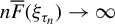 as
$n \to \infty $
 , the population expectile
$\xi _{\tau _n}$
 is extreme but well inside the sample so that it can be consistently estimated by its empirical version

where
$\eta _{\tau }(y)=|\tau -\mathbb {1} \{ y\leqslant 0 \}|y^2$
 , as described in Appendix A. In the more challenging extreme case when
$\tau = \tau ^{\prime }_n>\tau _n $
 such that
$(1-\tau _n)/(1-\tau ^{\prime }_n)\to \infty $
 as
$n \to \infty $
 , the population expectile
$\xi _{\tau ^{\prime }_n}$
 lies at the far tail of the underlying distribution, possibly beyond the sample maximum
$X_{n,n}$
 in the data. Using (2.3) with
$t=1/\overline {F}(\xi _{\tau _n})$
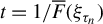 and
$x=\overline {F}(\xi _{\tau _n})/\overline {F}(\xi _{\tau ^{\prime }_n})$
 , and recalling that
$\lim _{t\to \infty } (U(1/\overline {F}(t))-t)/a(1/\overline {F}(t)) = 0$
 (see, e.g., the proof of Theorem B.3.19 in de Haan and Ferreira, Reference de Haan and Ferreira2006), we obtain the expectile-specific approximation

for n large enough. Since, in the heavy-tailed case with
$0<\gamma <1$
 , we have
$\overline {F}(\xi _{\tau })/(1-\tau ) \sim \gamma ^{-1}-1$
 as
$\tau \to 1$
 (Bellini et al., Reference Bellini, Klar, Müller and Gianin2014, Thm. 11), it follows that

as
$n\to \infty $
 , which in turn suggests the extrapolating approximation

Therefore, given estimators
$\breve {\sigma }_n$
 and
$\breve {\gamma }_n$
 of
$a(1/\overline {F}(\xi _{\tau _n}))$
 and
$\gamma $
 , respectively, this motivates the extreme expectile estimator

Various estimators of the scale function
$\sigma (\cdot )\equiv a(1/\overline {F}(\cdot ))$
 and shape parameter
$\gamma $
 are available in the literature, including the (pseudo-)GPML estimators and the Moment-type estimators: if
$k=k_n\to \infty $
 is a sequence of integers such that
$k/n\to 0$
 , as
$n\to \infty $
 , then
-
• The GPML estimators (Smith, Reference Smith1987; Drees et al., Reference Drees, Ferreira and de Haan2004) of $(a(n/k_n),\gamma )$
are given by $$\begin{align*}(\widehat{a}^{\mathrm{ML}}(n/k_n),\widehat{\gamma}_n^{\mathrm{ML}})=\operatorname*{\mbox{arg max}}_{\sigma,\gamma>0} \prod_{i=1}^{k_n} h(X_{n-i+1,n}-X_{n-k_n,n}|\sigma,\gamma), \end{align*}$$
where the Generalized Pareto density function is defined as $h(\cdot |\sigma ,\gamma )=H'(\cdot |\sigma ,\gamma )$
. -
• The Moment estimators (Dekkers et al., Reference Dekkers, Einmahl and de Haan1989) of $(a(n/k_n),\gamma )$
are defined as $$\begin{align*}\big(\widehat{a}^{\mathrm{Mom}}(n/k_n),\widehat{\gamma}_n^{\mathrm{Mom}}\big)&=\big(X_{n-k_n,n} M_{k_n}^{(1)} (1-\widehat{\gamma}_n^{(-)}), M_{k_n}^{(1)}+\widehat{\gamma}_n^{(-)}\big), \\ \text{where } \ \widehat{\gamma}_n^{(-)}&=1 - \frac{1}{2} \left( 1-\frac{(M_{k_n}^{(1)})^2}{M_{k_n}^{(2)}} \right)^{-1}\\ \text{and } \ M_{k_n}^{(j)}&=\frac{1}{{k_n}} \sum_{i=1}^{k_n} (\log X_{n-i+1,n}-\log X_{n-{k_n},n})^j, \ \text{ for } j=1,2. \end{align*} $$





Such estimators of the scale parameter
$a(1/\overline {F}(u_n))$
 typically converge on the relative scale at the rate
$1/\sqrt {n \overline {F}(u_n)}$
 (see Sections 3.4 and 4.2 in de Haan and Ferreira, Reference de Haan and Ferreira2006, for the i.i.d. case, and Section 6 in Drees, Reference Drees2003, for the case of dependent data). For
$u_n=\xi _{\tau _n}$
 , estimators
$\breve {\sigma }_n$
 of the parameter
$a(1/\overline {F}(\xi _{\tau _n}))$
 are therefore expected to converge on the relative scale at the rate
$1/\sqrt {n \overline {F}(\xi _{\tau _n})}$
 , which we have seen to be asymptotically proportional to the rate of convergence
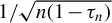
$1/\sqrt {n(1-\tau _n)}$
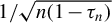 of the intermediate expectile estimator
$\widehat {\xi }_{\tau _n}$
 (see Theorem 2 below). It is also customary to use estimators
$\breve {\gamma }_n$
 that rely on the top
$k_n=n(1-\tau _n)$
 observations and converge at the same rate
$1/\sqrt {n(1-\tau _n)}$
 (see Sections 3.4–3.6 in de Haan and Ferreira, Reference de Haan and Ferreira2006, in the i.i.d. case, and Section 6 in Drees, Reference Drees2003, in the serially dependent case). A noteworthy difference between the GPML and Moment estimators is that the former are location- and scale-invariant, while the latter are only scale-invariant. This may be of importance in practical applications where the data are standardized and de-trended.
The next result shows that among the three estimators
$\widehat {\xi }_{\tau _n}$
 ,
$\breve {\gamma }_n$
 , and
$\breve {\sigma }_n$
 on which
$\breve {\xi }_{\tau ^{\prime }_n}^{\star }$
 hinges in (2.7), it is the asymptotic behavior of
$\breve {\gamma }_n$
 which dominates that of
$\breve {\xi }_{\tau ^{\prime }_n}^{\star }$
 .
Theorem 1. Assume that
-
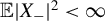
1. $\mathbb {E}|X_{-}|^2<\infty $
and
$\mathcal {E}_2(\gamma , \rho , a, A)$
holds with
$0 <\gamma <1/2$
and
$\rho < 0$
; -
2. $\tau _n=1-k_n/n \to 1$
such that
$n(1-\tau _n)=k_n \to \infty $
,
$\sqrt {n (1-\tau _n)} A((1-\tau _n)^{-1})\to \lambda _1\in \mathbb {R}$
,
$\sqrt {n (1-\tau _n)}/q_{\tau _n}\to \lambda _2\in \mathbb {R}$
, and
$\sqrt {n(1-\tau _n)} (a((1-\tau _n)^{-1})/q_{\tau _n} - \gamma ) \to \mu \in \mathbb {R}$
,
$n \to \infty $
; -
3. $\tau ^{\prime }_n \to 1$
such that
$(1-\tau _n)/(1-\tau ^{\prime }_n)\to \infty $
and
$\sqrt {n(1-\tau _n)}/\log ((1-\tau _n)/(1-\tau ^{\prime }_n)) \to \infty $
,
$n \to \infty $
; -
4. $\sqrt {n(1-\tau _n)}\left (\frac {\widehat {\xi }_{\tau _n}}{\xi _{\tau _n}}-1\right ) = \mathrm {O}_{\mathbb {P}}(1)$
and for suitable estimators
$\breve {\gamma }_n$
and
$\breve {\sigma }_n$
, $$\begin{align*}\sqrt{n(1-\tau_n)} \left( \frac{\breve{\sigma}_n}{a(1/\overline{F}(\xi_{\tau_n}))} - 1 \right) = \mathrm{O}_{\mathbb{P}}(1) \ \text{ and } \ \sqrt{n(1-\tau_n)} (\breve{\gamma}_n-\gamma)\stackrel{\mathrm{d}}{\longrightarrow} \Gamma, \end{align*}$$
where $\Gamma $
is a nondegenerate limit.
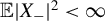
















Then

Under the i.i.d. model assumption, the property
$\sqrt {n(1-\tau _n)}\left (\frac {\widehat {\xi }_{\tau _n}}{\xi _{\tau _n}}-1\right ) = \mathrm {O}_{\mathbb {P}}(1)$
 follows immediately from the asymptotic normality of
$\widehat {\xi }_{\tau _n}$
 derived in Theorem 1 of Daouia et al. (Reference Daouia, Girard and Stupfler2020) when
$0<\gamma <1/2$
 and
$\mathbb {E}|X_{-}|^2<\infty $
 . Note also that by Corollary 4.3.2 on p. 135 in de Haan and Ferreira (Reference de Haan and Ferreira2006), the conditions of our Theorem 1 imply

which is useful for constructing an asymptotic confidence interval for
$\xi _{\tau ^{\prime }_n}$
 . For this same purpose and for the calculation of
$\breve {\xi }_{\tau ^{\prime }_n}^{\star }$
 in (2.7), the estimator
$\breve {\sigma }_n$
 of
$a(1/\overline {F}(\xi _{\tau _n}))$
 can be obtained in three different ways by setting

The first estimator
$\breve {\sigma }^{(1)}_n$
 is simply the empirical counterpart of
$a(1/\overline {F}(\xi _{\tau _n}))$
 . The second estimator
$\breve {\sigma }^{(2)}_n$
 is obtained in view of the approximation
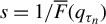
$a(1/\overline {F}(\xi _{\tau _n})) \approx a((1-\tau _n)^{-1}) \times ((1-\tau _n)/\overline {F}(\xi _{\tau _n}))^{\gamma }$
 that follows from the regular variation property
$\lim _{s\to \infty }a(sz)/a(s)=z^{\gamma }$
 , for any
$z>0$
 (see Lemma 1.2.9 on page 22 in de Haan and Ferreira, Reference de Haan and Ferreira2006), when taking
$s=1/\overline {F}(q_{\tau _n})$
 and
$z=\overline {F}(q_{\tau _n})/\overline {F}(\xi _{\tau _n})$
 . The third estimator
$\breve {\sigma }^{(3)}_n$
 is obtained from the same approximation above by replacing
$\overline {F}(\xi _{\tau _n})/(1-\tau _n)$
 with its limit
$\gamma ^{-1}-1$
 . These three versions of
$\breve {\sigma }_n$
 will be denoted in the sequel as
$\breve {\sigma }_n^{\mathrm {ML},i},\, i=1,2,3$
 , when using the GPML method and as
$\breve {\sigma }_n^{\mathrm {Mom},i},\, i=1,2,3$
 , when using the Moment method. This will in turn result in the associated GPML-based expectile estimators
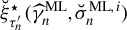
$\breve {\xi }_{\tau ^{\prime }_n}^{\star }(\widehat {\gamma }_n^{\mathrm {ML}},\breve {\sigma }_n^{\mathrm {ML},i})$
 and Moment-type estimators
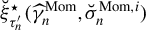
$\breve {\xi }_{\tau ^{\prime }_n}^{\star }(\widehat {\gamma }_n^{\mathrm {Mom}},\breve {\sigma }_n^{\mathrm {Mom},i})$
 . These estimators can be calculated by using our function gpdExpect from the R package Expectrem with the respective methods "direct_ML1"
$,\ldots ,$
 "direct_ML3", and "direct_MOM1"
$,\ldots ,$
 "direct_MOM3".
It is also natural and instructive to compare Theorem 1 with the results for the competing Weissman-type estimators reviewed in Appendix A. We have from the proof of Theorem 1 the following equivalent statement:

Therefore,
$\breve {\xi }_{\tau ^{\prime }_n}^{\star }$
 has the same rate of convergence as
$\widetilde {\xi }^\star _{\tau ^{\prime }_n}$
 in (A.6) and
$\widehat {\xi }^\star _{\tau ^{\prime }_n}$
 in (A.7), as well as their bias-corrected versions
$\widehat {\xi }_{\tau ^{\prime }_n}^{\star ,\mathrm {BR}}$
 in (B.5) and
$\widetilde {\xi }_{\tau ^{\prime }_n}^{\star ,\mathrm {BR}}$
 in (B.6). While the asymptotic distribution
$\Gamma $
 of these Weissman-type estimators is typically that of the Hill estimator
$\widehat {\gamma }_{n}^{\mathrm {H}}$
 or the expectile-based estimator
$\widehat {\gamma }_{n}^{\mathrm {E}}$
 in (A.3), or their bias-reduced versions
$\widehat {\gamma }_{n}^{\mathrm {H},\mathrm {BR}}$
 and
$\widehat {\gamma }_{n}^{\mathrm {E},\mathrm {BR}}$
 in (A.10) and (A.11), it would naturally correspond in our generalized Pareto approach to the limit distribution of the GPML estimator
$\widehat {\gamma }_n^{\mathrm {ML}}$
 or Moment estimator
$\widehat {\gamma }_n^{\mathrm {Mom}}$
 . Interestingly, the GPML and Moment methods often correct for bias and can be more robust in small and moderate samples or when the optimal
$k_n$
 selection is unclear from Hill plots. Selection of the threshold
$k_n$
 is known to be a difficult task in general. Schneider, Krajina, and Krivobokova (Reference Schneider, Krajina and Krivobokova2021) develop two threshold selection methods under the assumption that
$\gamma>0$
 and compare them with eight competitors, including bootstrap techniques. Approaches that are specifically tailored to GP models are the changepoint tests of Northrop and Coleman (Reference Northrop and Coleman2014) and the simultaneous threshold stability plots of Wadsworth (Reference Wadsworth2016) based on point process calculations. The latter two methods are implemented in the R package mev developed by Belzile et al. (Reference Belzile, Wadsworth, Northrop, Huser, Grimshaw, Zhang, Stephens and Owen2025). In our simulation study (Section 3), we shall examine the performance of our estimators as functions of the threshold, so as to find the best performers across a large range of threshold values; our financial real data analysis (Section 4) will use a simple selection rule based on finding the best extreme expectile forecast across time.
When the data follow a GPD,
$\widehat {\gamma }_n^{\mathrm {ML}}$
 is the estimator that tends to achieve the lowest mean squared error (MSE) in moderate to large samples, but can be unstable for small samples. The estimator
$\widehat {\gamma }_n^{\mathrm {Mom}}$
 is more robust when
$\widehat {\gamma }_n^{\mathrm {ML}}$
 becomes unstable, while still being competitive in terms of variance (see, e.g., Beirlant et al., Reference Beirlant, Goegebeur, Segers and Teugels2004, and Yılmaz, Kara, and Özdemir, Reference Yılmaz, Kara and Özdemir2021, for a detailed comparison and review on estimation procedures for the EVI). The preference for
$\breve {\xi }_{\tau ^{\prime }_n}^{\star }$
 over the Weissman-type competitors stems not only from such practical advantages of the EVI estimators
$\widehat {\gamma }_n^{\mathrm {ML}}$
 and
$\widehat {\gamma }_n^{\mathrm {Mom}}$
 over the Hill-based alternatives, but also from its reliance on additional location parameter estimates that contribute to capturing uncertainty more effectively. Our experience with real and simulated heavy-tailed profit–loss data shows that, across a wide range of
$k_n$
 values and without finite-sample correction,
$\breve {\xi }_{\tau ^{\prime }_n}^{\star }$
 stands out as the best performer in terms of smoothness and stability for moderate-sized datasets, but also in terms of relative bias and mean-squared error, with its Gaussian asymptotic confidence intervals attaining coverage closer to the nominal level (because it fits the exceedances over a threshold using a parametric model, whereas the nonparametric Weissman estimators are more data-driven and require large samples to provide accurate estimates). We will specialize the discussion of our generic Theorem 1 to both shape parameter estimators
$\breve {\gamma }_n\in \{\widehat {\gamma }_n^{\mathrm {ML}}, \widehat {\gamma }_n^{\mathrm {Mom}}\}$
 in Section 2.4 when the scale parameter estimator takes the form
$\breve {\sigma }_n:=\breve {\sigma }^{(3)}_n = \widehat {a}((1-\tau _n)^{-1}) \, (\breve {\gamma }_n^{-1}-1)^{-\breve {\gamma }_n}$
 , with
$\widehat {a}(\cdot )\in \{\widehat {a}^{\mathrm {ML}}(\cdot ), \widehat {a}^{\mathrm {Mom}}(\cdot )\}$
 . This choice of
$\breve {\sigma }_n$
 is motivated by its good performance in our numerical illustrations; one could, analogously, state a result for
$\breve {\sigma }_n:=\breve {\sigma }^{(2)}_n$
 given the
$\sqrt {n(1-\tau _n)}$
 -convergence of
$\widehat {\overline {F}}_n(\widehat {\xi }_{\tau _n})$
 (which, in the i.i.d. setting, follows from a Gaussian approximation to the tail empirical process, see, e.g., Theorem 5.1.2 on page 159 in de Haan and Ferreira, Reference de Haan and Ferreira2006), and for
$\breve {\sigma }_n:=\breve {\sigma }^{(1)}_n$
 given a specific, explicit form of the estimator
$\widehat {a}(\cdot )$
 . Next, we show that its associated assumption in Theorem 1 holds under convenient conditions on both
$\breve {\gamma }_n$
 and
$\widehat {a}((1-\tau _n)^{-1})$
 .
Theorem 2. Assume that
-
1. $\mathbb {E}|X_{-}|<\infty $
and
$\mathcal {E}_2(\gamma , \rho , a, A)$
holds with
$0 <\gamma <1$
and
$\rho < 0$
; -
2. $\tau _n\uparrow 1$
such that
$n(1-\tau _n) \to \infty $
,
$\sqrt {n (1-\tau _n)} A((1-\tau _n)^{-1})=\mathrm {O}(1)$
,
$\sqrt {n (1-\tau _n)}/ q_{\tau _n}=\mathrm {O}(1)$
, and
$\sqrt {n(1-\tau _n)} (a((1-\tau _n)^{-1})/q_{\tau _n} - \gamma ) = \mathrm {O}(1)$
,
$n \to \infty $
.









Take
$\breve {\sigma }_n = \widehat {a}((1-\tau _n)^{-1}) \times (\breve {\gamma }_n^{-1}-1)^{-\breve {\gamma }_n}$
 for suitable estimators
$\widehat {a}((1-\tau _n)^{-1})$
 and
$\breve {\gamma }_n$
 such that

where
$\Gamma $
 is a nondegenerate limit. Then

In the financial context of real-valued profit–loss heavy-tailed distributions, we provide Monte Carlo evidence in Section 3 that, at least, our GPML estimator
$\breve {\xi }_{\tau ^{\prime }_n}^{\star }(\widehat {\gamma }_n^{\mathrm {ML}},\breve {\sigma }_n^{\mathrm {ML},2})$
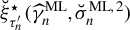 outperforms the best-known Weissman competitors among those described in Appendix A, both in terms of relative bias and mean-squared error, with its associated asymptotic confidence interval having slightly better coverage at the expense of being wider.
2.3 Extremal Quantile-Based Estimation
Using now (2.3) with
$t=(1-\tau _n)^{-1}$
 and
$x=(1-\tau _n)/(1-\tau ^{\prime }_n)$
 leads to the well-known Generalized Pareto quantile approximation

for all n large enough, which results in the extrapolated extreme quantile estimator

for suitable estimators
$\widehat {\sigma }_n$
 and
$\widehat {\gamma }_n$
 of the scale and shape parameters
$a((1-\tau _n)^{-1})$
 and
$\gamma $
 , respectively. In our heavy-tailed model (
$\gamma>0$
 ), the asymptotic connection
$\xi _{\tau ^{\prime }_n}\sim (\gamma ^{-1}-1)^{-\gamma }{q_{\tau ^{\prime }_n}}$
 from (2.5) motivates then the quantile-based estimator

for
$\xi _{\tau ^{\prime }_n}$
 , which extrapolates the intermediate expectile estimator
$\check {\xi }_{\tau _n}:=(\widehat {\gamma }_n^{-1}-1)^{-\widehat {\gamma }_n}\widehat {q}_{\tau _n}$
 to the far tail at
$\tau ^{\prime }_n$
 . Next, we establish the asymptotic distribution of this new GPD-type estimator for generic estimators
$\widehat {\gamma }_n$
 and
$\widehat {\sigma }_n$
 of the shape and scale parameters.
Theorem 3. Assume that
-
1. $\mathbb {E}|X_{-}|<\infty $
and
$\mathcal {E}_2(\gamma , \rho , a, A)$
holds with
$0 <\gamma <1$
and
$\rho < 0$
; -
2. $\tau _n=1-k_n/n \to 1$
such that
$n(1-\tau _n)=k_n \to \infty $
,
$\sqrt {n (1-\tau _n)} A((1-\tau _n)^{-1})\to \lambda _1\in \mathbb {R}$
,
$\sqrt {n (1-\tau _n)}/q_{\tau _n}\to \lambda _2\in \mathbb {R}$
, and
$\sqrt {n(1-\tau _n)} (a((1-\tau _n)^{-1})/q_{\tau _n} - \gamma ) \to \mu \in \mathbb {R}$
,
$n \to \infty $
; -
3. $\tau ^{\prime }_n \to 1$
such that
$(1-\tau _n)/(1-\tau ^{\prime }_n)\to \infty $
and
$\sqrt {n(1-\tau _n)}/\log ((1-\tau _n)/(1-\tau ^{\prime }_n)) \to \infty $
,
$n \to \infty $
; -
4. for suitable estimators $\widehat {\gamma }_n$
of
$\gamma $
and
$\widehat {\sigma }_n$
of
$\sigma (q_{\tau _n})= a((1-\tau _n)^{-1})$
, (2.10) $$ \begin{align} \sqrt{n(1-\tau_n)}\left( \widehat{\gamma}_n-\gamma, \frac{\widehat{\sigma}_n}{\sigma(q_{\tau_n})}-1, \frac{\widehat{q}_{\tau_n}-q_{\tau_n}}{\sigma(q_{\tau_n})} \right) \stackrel{\mathrm{d}}{\longrightarrow} (\Gamma, \Lambda, B), \end{align} $$
where $(\Gamma , \Lambda , B)$
is a nontrivial trivariate weak limit.


















Then

As can be seen from the proof of Theorem 3, an equivalent statement of this convergence is

which yields exactly the same rate of convergence as the competing Weissman-type estimators seen in Appendix A. Similarly to these estimators, it is the asymptotic distribution
$\Gamma $
 of the chosen tail index estimator
$\widehat {\gamma }_n$
 which dominates the limit distribution of our extreme expectile estimator
$\check {\xi }^\star _{\tau ^{\prime }_n}(\widehat {\gamma }_n,\widehat {\sigma }_n)$
 . In Section 2.4 below, we shall specialize the discussion of Theorem 3 to the GPML and Moment-type estimators
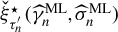
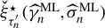
$\check {\xi }_{\tau ^{\prime }_n}^{\star }(\widehat {\gamma }_n^{\mathrm {ML}},\widehat {\sigma }_n^{\mathrm {ML}})$
 and
$\check {\xi }_{\tau ^{\prime }_n}^\star (\widehat {\gamma }_n^{\mathrm {Mom}},\widehat {\sigma }_n^{\mathrm {Mom}})$
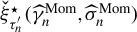 obtained by taking the estimators
$\widehat {\gamma }_n$
 and
$\widehat {\sigma }_n$
 in (2.9) for the shape and scale parameters
$\gamma $
 and
$\sigma (q_{\tau _n})\equiv a(n/k_n)$
 to be either
$\widehat {\gamma }_n^{\mathrm {ML}}$
 and
$\widehat {\sigma }_n^{\mathrm {ML}}$
 or
$\widehat {\gamma }_n^{\mathrm {Mom}}$
 and
$\widehat {\sigma }_n^{\mathrm {Mom}}$
 , respectively, where

The two extrapolated estimators
$\check {\xi }_{\tau ^{\prime }_n}^{\star }(\widehat {\gamma }_n^{\mathrm {ML}},\widehat {\sigma }_n^{\mathrm {ML}})$
 and
$\check {\xi }_{\tau ^{\prime }_n}^\star (\widehat {\gamma }_n^{\mathrm {Mom}},\widehat {\sigma }_n^{\mathrm {Mom}})$
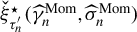 can be calculated by using the function gpdExpect from the R package Expectrem, with method="indirect_ML" and method="indirect_MOM", respectively. Our simulation study in Section 3 indicates that their finite-sample performance is very similar to that of the third direct GPML and Moment estimators
$\breve {\xi }_{\tau ^{\prime }_n}^{\star }(\widehat {\gamma }_n^{\mathrm {ML}},\breve {\sigma }_n^{\mathrm {ML},3})$
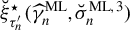 and
$\breve {\xi }_{\tau ^{\prime }_n}^{\star }(\widehat {\gamma }_n^{\mathrm {Mom}},\breve {\sigma }_n^{\mathrm {Mom},3})$
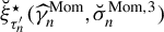 , respectively (as the only difference lies, by construction, between their related intermediate direct and indirect expectile estimators). Moreover, in the case of nonnegative loss distributions, the Moment-type estimator
$\check {\xi }_{\tau ^{\prime }_n}^{\star }(\widehat {\gamma }_n^{\mathrm {Mom}},\widehat {\sigma }_n^{\mathrm {Mom}})$
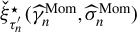 shows competitive relative mean-squared errors with remarkably lower relative bias estimates than those of the bias-corrected Weissman estimators. In the case of real-valued profit–loss distributions, this indirect Moment estimator still posts respectable results for low values of
$\gamma $
 , but the direct GPML estimator
$\breve {\xi }_{\tau ^{\prime }_n}^{\star }(\widehat {\gamma }_n^{\mathrm {ML}},\breve {\sigma }_n^{\mathrm {ML},2})$
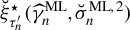 stands out in terms of relative mean-squared errors and coverage probabilities of its associated confidence interval, exhibiting consistent results over all values of
$\gamma $
 .
2.4 GPML and Moment-Type Estimators
In this section, we focus the discussion of the asymptotic theory on the GPML and Moment estimators
$(\widehat {a}^{\mathrm {ML}}(n/k_n),\widehat {\gamma }_n^{\mathrm {ML}})$
 and
$\big (\widehat {a}^{\mathrm {Mom}}(n/k_n),\widehat {\gamma }_n^{\mathrm {Mom}}\big )$
 of the scale and shape parameters
$(a(n/k_n),\gamma )$
 , for the discretized intermediate level
$\tau _n =1-k_n/n$
 with
$k_n \to \infty $
 and
$k_n/n \to 0$
 as
$n\to \infty $
 . Although our generic Theorems 1–3 are valid in a general setup allowing for serial dependency in the data, we impose an i.i.d. assumption on the underlying sample.
We first consider the extrapolated asymmetric least squares estimators
$\breve {\xi }_{\tau ^{\prime }_n}^{\star }(\widehat {\gamma }_n^{\mathrm {ML}},\breve {\sigma }_n^{\mathrm {ML}})$
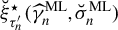 and
$\breve {\xi }_{\tau ^{\prime }_n}^{\star }(\widehat {\gamma }_n^{\mathrm {Mom}},\breve {\sigma }_n^{\mathrm {Mom}})$
 defined in (2.7) by taking therein the estimators
$\breve {\gamma }_n$
 and
$\breve {\sigma }_n$
 of the shape and scale parameters
$\gamma $
 and
$\sigma (\xi _{\tau _n})\equiv a(1/\overline {F}(\xi _{\tau _n}))$
 to be either
$\widehat {\gamma }_n^{\mathrm {ML}}$
 and
$\breve {\sigma }_n^{\mathrm {ML}}$
 or
$\widehat {\gamma }_n^{\mathrm {Mom}}$
 and
$\breve {\sigma }_n^{\mathrm {Mom}}$
 , respectively, with

Following Theorem 3.4.2 on p. 92 in de Haan and Ferreira (Reference de Haan and Ferreira2006) and the asymptotic independence between functions of the stochastic process
$(X_{n-\lfloor k_ns \rfloor ,n}-X_{n-k_n,n})_{0<s\leq 1}$
 and the random variable
$X_{n-k_n,n}$
 (see, e.g., Corollary 2.4.6 on page 52 in de Haan and Ferreira, Reference de Haan and Ferreira2006), the GPML estimators
$\widehat {\gamma }_n^{\mathrm {ML}}$
 and
$\widehat {\sigma }_n^{\mathrm {ML}}$
 satisfy, under the second-order condition
$\mathcal {E}_2(\gamma , \rho , a, A)$
 with
$\gamma>0$
 and the bias condition
$\sqrt {k_n}A(n/k_n)\to \lambda _1\in \mathbb {R}$
 , the joint convergence

where
$b^{\mathrm {ML}}=\left ( \frac {\gamma +1}{(1-\rho )(1+\gamma -\rho )}, \frac {-\rho }{(1-\rho )(1+\gamma -\rho )}, 0 \right )$
 and the matrix
$\Sigma ^{\mathrm {ML}}$
 is given by

Under the extra condition
$\sqrt {n(1-\tau _n)} (a((1-\tau _n)^{-1})/q_{\tau _n} - \gamma ) \to \mu \in \mathbb {R}$
 , it can be seen from Corollary 4.2.2 on p. 133 in de Haan and Ferreira (Reference de Haan and Ferreira2006) that the Moment estimators
$\widehat {\gamma }_n^{\mathrm {Mom}}$
 and
$\widehat {\sigma }_n^{\mathrm {Mom}}$
 satisfy the joint convergence

where

Note that the asymptotic variance of
$\widehat {\gamma }_n^{\mathrm {Mom}}$
 is lower than that of
$\widehat {\gamma }_n^{\mathrm {ML}}$
 , but the analysis of the respective biases of these two estimators, and therefore a definitive comparison of their finite-sample performance, is more complex. With the convergence results (2.12) and (2.13) at hand, we show that the two direct extreme expectile estimators
$\breve {\xi }_{\tau ^{\prime }_n}^{\star }(\widehat {\gamma }_n^{\mathrm {ML}},\breve {\sigma }_n^{\mathrm {ML}})$
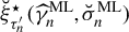 and
$\breve {\xi }_{\tau ^{\prime }_n}^{\star }(\widehat {\gamma }_n^{\mathrm {Mom}},\breve {\sigma }_n^{\mathrm {Mom}})$
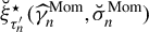 are asymptotically normal.
Corollary 1. Under the first three conditions of Theorem 1, and provided the data are i.i.d., we have

Turning to the indirect quantile-based estimators
$\check {\xi }^\star _{\tau ^{\prime }_n}(\widehat {\gamma }_n^{\mathrm {ML}},\widehat {\sigma }_n^{\mathrm {ML}})$
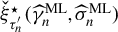 and
$\check {\xi }^\star _{\tau ^{\prime }_n}(\widehat {\gamma }_n^{\mathrm {Mom}},\widehat {\sigma }_n^{\mathrm {Mom}})$
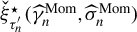 defined in (2.9), we obtain the following asymptotic normality results.
Corollary 2. Under the first three conditions of Theorem 3, and provided the data are i.i.d., we have

In order to keep the article to manageable proportions, we do not discuss the application of our theorems and all the associated ramifications in the presence of dependence in the data. Similarly to extreme quantile estimation under mixing conditions (Drees, Reference Drees2003) or ARMA-GARCH models (He et al., Reference He, Peng, Zhang and Zhao2022), our methods may work under serial dependence with an increased asymptotic variance. Theoretical results along these lines are left for future research. In our case study of financial time series, we consider a practical solution to eliminate serial dependence by filtering the time series with an ARMA-GARCH model. The residuals from the fitted model are then treated as i.i.d. after performing a series of Ljung–Box independence tests on residuals and their squares.
3 SIMULATION STUDY
We evaluate the performance of our extreme expectile estimators through an extensive simulation study. We consider two nonnegative loss distributions and two real-valued profit–loss distributions for the distribution of X, all with tail index
$\gamma>0$
 :
-
• Fréchet distribution with survival function $\overline {F}(x) = 1 - \exp \left (-x^{-1/\gamma }\right )$
for
$x>0$
; -
• Burr distribution with survival function $\overline {F}(x) = 1/(1+x^{1/\gamma })$
for
$x>0$
; -
• Symmetric Burr distribution with density function $\ f(x)=\tfrac {1}{2\gamma }\tfrac {|x|^{1/\gamma -1}}{(1+|x|^{1/\gamma })^2}$
for
$x\in \mathbb {R}$
; -
• Student distribution with degrees of freedom $1/\gamma $
.




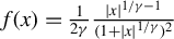


The first two nonnegative distributions are commonly seen in insurance applications, while the latter two real-valued distributions are more suitable for financial returns. For each distribution, we examine the cases
$\gamma = 0.25$
 , 0.3, 0.35, and 0.4 for all competing estimators

where
$i \in \{1,2,3\}$
 and
$\widehat {\xi }_{\tau ^{\prime }_n}$
 is the naive, non-extrapolated empirical expectile estimator described in (2.6) at level
$\tau ^{\prime }_n$
 . The choice of
$\gamma $
 values between 0.25 and 0.4 describes quite well the tail heaviness of most financial datasets (see, e.g., the R package CASdatasets). We generate
$B = 5{,}000$
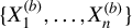
 samples
$\{X^{(b)}_1, \ldots , X^{(b)}_n\}$
 for
$b=1,\ldots ,B$
 , with
$n=1{,}500$
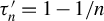
 in each simulation case, and estimate the extreme expectile
$\xi _{\tau _n'}$
 at the level
$\tau _n' = 1 - 1/n$
 , where
$\xi _{\tau _n'}$
 is of the same order of magnitude as the sample maximum
$X_{n,n}$
 . We compare the finite-sample performance of the different estimators based on the following criteria:
-
1. Relative bias and mean-squared errors
$$ \begin{align*}\mathrm{RBias}(\overline{\xi}_{\tau_n'}) = \dfrac{1}{B} \sum_{b=1}^B\left(\dfrac{\overline{\xi}_{\tau_n'}^{(b)}}{\xi_{\tau_n'}}-1\right) \ \text{ and } \ \mathrm{RMSE}(\overline{\xi}_{\tau_n'}) = \dfrac{1}{B} \sum_{b=1}^B\left(\dfrac{\overline{\xi}_{\tau_n'}^{(b)}}{\xi_{\tau_n'}}-1\right)^2, \end{align*} $$
where $\overline {\xi }_{\tau _n'}^{(b)}$
is the expectile estimator generated from the bth sample. -
2. Average length and coverage probability of the $95\%$
asymptotic Gaussian confidence intervals, where the former is defined as the average width of the confidence intervals generated around each estimator, and the latter is the frequency of times said intervals included the true value of the extreme expectile.


We plot the estimates of
$\mathrm {RBias}(\overline {\xi }_{\tau _n'})$
 and
$\mathrm {RMSE}(\overline {\xi }_{\tau _n'})$
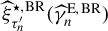
 against k for the positive-valued distributions in Figure 1, and those for the real-valued distributions in Figure 2. Figure 1 reveals that the BR (Bias-reduced) and PS (Padoan and Stupfler, Reference Padoan and Stupfler2022) estimators
$\widehat {\xi }_{\tau ^{\prime }_n}^{\star ,\mathrm {BR}}(\widehat {\gamma }_{n}^{\mathrm {E},\mathrm {BR}})$
 ,
$\widetilde {\xi }_{\tau ^{\prime }_n}^{\star ,\mathrm {BR}}(\widehat {\gamma }_{n}^{\mathrm {H},\mathrm {BR}})$
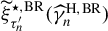 ,
$\widehat {\xi }_{\tau ^{\prime }_n}^{\star ,\mathrm {PS}}$
 , and
$\widetilde {\xi }_{\tau ^{\prime }_n}^{\star ,\mathrm {PS}}$
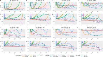
 , seen in Appendix B and represented as solid lines in the figure, perform well in the positive-valued cases of the Fréchet and Burr distributions. However, the Burr distribution also sees our two direct GPML estimators
$\breve {\xi }_{\tau ^{\prime }_n}^{\star }(\widehat {\gamma }_n^{\mathrm {ML}},\breve {\sigma }_n^{\mathrm {ML},1})$
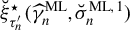 and
$\breve {\xi }_{\tau ^{\prime }_n}^{\star }(\widehat {\gamma }_n^{\mathrm {ML}},\breve {\sigma }_n^{\mathrm {ML},2})$
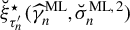 , represented, respectively, by the dashed turquoise and purple lines, reach similar RMSE levels to their BR and PS competitors, but for narrower ranges of k values that are typically higher than the optimal k values for the BR and PS families of estimators. Our indirect and third direct Moment estimators
$\check {\xi }_{\tau ^{\prime }_n}^{\star }(\widehat {\gamma }_n^{\mathrm {Mom}},\widehat {\sigma }_n^{\mathrm {Mom}})$
 and
$\breve {\xi }_{\tau ^{\prime }_n}^{\star }(\widehat {\gamma }_n^{\mathrm {Mom}},\breve {\sigma }_n^{\mathrm {Mom},3})$
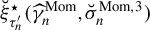 , shown in dash-dotted blue and dashed pink, respectively, shore up this shortcoming by maintaining competitive RMSE measures over long ranges of k values for both the Fréchet and Burr distributions and low RBias estimates for both distributions and all values of
$\gamma $
 .
Simulation results for positive-valued distributions. Panels (a)–(d) and (e)–(h) show the Monte-Carlo estimates of RMSE and RBias, respectively, for the Fréchet distribution, while panels (i)–(l) and (m)–(p) show those for the Burr distribution. Each group of four panels is ordered by tail index value
$\gamma \in \{0.25, 0.3, 0.35, 0.4\}$
 . For
$n=1{,}500$
 and
$\tau _n' = 1 - 1/n$
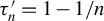 , we consider the naive empirical estimator
$\widehat {\xi }_{\tau ^{\prime }_n}$
 (Empirical), the direct BR and PS estimators
$\widehat {\xi }_{\tau ^{\prime }_n}^{\star ,\mathrm {BR}}(\widehat {\gamma }_{n}^{\mathrm {E},\mathrm {BR}})$
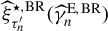 (ALS-BR) and
$\widehat {\xi }_{\tau ^{\prime }_n}^{\star ,\mathrm {PS}}$
 (ALS-PS), their indirect counterparts
$\widetilde {\xi }_{\tau ^{\prime }_n}^{\star ,\mathrm {BR}}(\widehat {\gamma }_{n}^{\mathrm {H},\mathrm {BR}})$
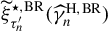 (QB-BR) and
$\widetilde {\xi }_{\tau ^{\prime }_n}^{\star ,\mathrm {PS}}$
 (QB-PS), our direct GPML estimators
$\breve {\xi }_{\tau ^{\prime }_n}^{\star }(\widehat {\gamma }_n^{\mathrm {ML}},\breve {\sigma }_n^{\mathrm {ML},1})$
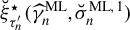 (ALS1-ML),
$\breve {\xi }_{\tau ^{\prime }_n}^{\star }(\widehat {\gamma }_n^{\mathrm {ML}},\breve {\sigma }_n^{\mathrm {ML},2})$
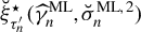 (ALS2-ML), and
$\breve {\xi }_{\tau ^{\prime }_n}^{\star }(\widehat {\gamma }_n^{\mathrm {ML}},\breve {\sigma }_n^{\mathrm {ML},3})$
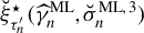 (ALS3-ML), the direct Moment estimators
$\breve {\xi }_{\tau ^{\prime }_n}^{\star }(\widehat {\gamma }_n^{\mathrm {Mom}},\breve {\sigma }_n^{\mathrm {Mom},1})$
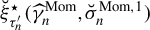 (ALS1-Mom),
$\breve {\xi }_{\tau ^{\prime }_n}^{\star }(\widehat {\gamma }_n^{\mathrm {Mom}},\breve {\sigma }_n^{\mathrm {Mom},2})$
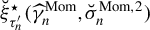 (ALS2-Mom), and
$\breve {\xi }_{\tau ^{\prime }_n}^{\star }(\widehat {\gamma }_n^{\mathrm {Mom}},\breve {\sigma }_n^{\mathrm {Mom},3})$
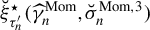 (ALS3-Mom), and the indirect GPML and Moment estimators
$\check {\xi }_{\tau ^{\prime }_n}^{\star }(\widehat {\gamma }_n^{\mathrm {ML}},\widehat {\sigma }_n^{\mathrm {ML}})$
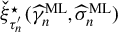 (QB-ML) and
$\check {\xi }_{\tau ^{\prime }_n}^{\star }(\widehat {\gamma }_n^{\mathrm {Mom}},\widehat {\sigma }_n^{\mathrm {Mom}})$
 (QB-Mom).

Figure 1 Long description
A grid of 16 line graphs arranged in a 4 by 4 layout.
Row 1 (panels a to d): R M S E for Frechet distribution with gamma values 0.25, 0.30, 0.35, and 0.40. The x-axis represents k from 0 to 1500. Most estimators show a U-shaped curve, starting high, dipping to a minimum between k equals 250 and 750, and then rising sharply. The Empirical estimator (solid red line) remains constant and horizontal across all k.
Row 2 (panels e to h): R Bias for Frechet distribution. The y-axis ranges from negative 0.50 to 0.50. Most curves start near zero, fluctuate slightly, and then diverge as k increases. A L S-G P D and Q B-G P D estimators (dashed lines in blue, purple, and pink) tend to trend downward into negative bias at high k, while A L S-B R and A L S-P S (solid green lines) trend upward.
Row 3 (panels i to l): R M S E for Burr distribution. Similar to Row 1, curves exhibit U-shapes. As gamma increases from 0.25 to 0.40, the minimum R M S E point for most estimators shifts slightly to the right and the curves become more compressed vertically.
Row 4 (panels m to p): R Bias for Burr distribution. Similar to Row 2, showing the divergence of estimators at higher k values. The Empirical estimator is a flat red line slightly below zero.
Legend at the bottom categorizes estimators into Competitors (Empirical, Q B-B R, A L S-B R, Q B-P S, A L S-P S), A L S-G P D (A L S 1-M L, A L S 1-Mom, A L S 2-M L, A L S 2-Mom, A L S 3-M L, A L S 3-Mom), and Q B-G P D (Q B-M L, Q B-Mom). Line styles include solid and various dashed patterns in a spectrum of colors from red and orange to green, blue, and magenta.
Simulation results for real-valued distributions. Panels (a)–(d) and (e)–(h) show the Monte-Carlo estimates of RMSE and RBias, respectively, for the symmetric Burr distribution, while panels (i)–(l) and (m)–(p) show those for the Student distribution. Each group of four panels is ordered by tail index value
$\gamma \in \{0.25, 0.3, 0.35, 0.4\}$
 . For
$n=1{,}500$
 and
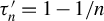
$\tau _n' = 1 - 1/n$
 , we consider the naive empirical estimator
$\widehat {\xi }_{\tau ^{\prime }_n}$
 (Empirical), the direct BR and PS estimators
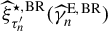
$\widehat {\xi }_{\tau ^{\prime }_n}^{\star ,\mathrm {BR}}(\widehat {\gamma }_{n}^{\mathrm {E},\mathrm {BR}})$
 (ALS-BR) and
$\widehat {\xi }_{\tau ^{\prime }_n}^{\star ,\mathrm {PS}}$
 (ALS-PS), their indirect counterparts
$\widetilde {\xi }_{\tau ^{\prime }_n}^{\star ,\mathrm {BR}}(\widehat {\gamma }_{n}^{\mathrm {H},\mathrm {BR}})$
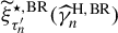 (QB-BR) and
$\widetilde {\xi }_{\tau ^{\prime }_n}^{\star ,\mathrm {PS}}$
 (QB-PS), our direct GPML estimators
$\breve {\xi }_{\tau ^{\prime }_n}^{\star }(\widehat {\gamma }_n^{\mathrm {ML}},\breve {\sigma }_n^{\mathrm {ML},1})$
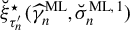 (ALS1-ML),
$\breve {\xi }_{\tau ^{\prime }_n}^{\star }(\widehat {\gamma }_n^{\mathrm {ML}},\breve {\sigma }_n^{\mathrm {ML},2})$
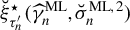 (ALS2-ML), and
$\breve {\xi }_{\tau ^{\prime }_n}^{\star }(\widehat {\gamma }_n^{\mathrm {ML}},\breve {\sigma }_n^{\mathrm {ML},3})$
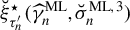 (ALS3-ML), the direct Moment estimators
$\breve {\xi }_{\tau ^{\prime }_n}^{\star }(\widehat {\gamma }_n^{\mathrm {Mom}},\breve {\sigma }_n^{\mathrm {Mom},1})$
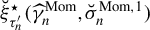 (ALS1-Mom),
$\breve {\xi }_{\tau ^{\prime }_n}^{\star }(\widehat {\gamma }_n^{\mathrm {Mom}},\breve {\sigma }_n^{\mathrm {Mom},2})$
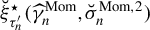 (ALS2-Mom), and
$\breve {\xi }_{\tau ^{\prime }_n}^{\star }(\widehat {\gamma }_n^{\mathrm {Mom}},\breve {\sigma }_n^{\mathrm {Mom},3})$
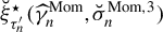 (ALS3-Mom), and the indirect GPML and Moment estimators
$\check {\xi }_{\tau ^{\prime }_n}^{\star }(\widehat {\gamma }_n^{\mathrm {ML}},\widehat {\sigma }_n^{\mathrm {ML}})$
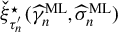 (QB-ML) and
$\check {\xi }_{\tau ^{\prime }_n}^{\star }(\widehat {\gamma }_n^{\mathrm {Mom}},\widehat {\sigma }_n^{\mathrm {Mom}})$
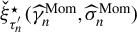 (QB-Mom).

Figure 2 Long description
The figure consists of a 4 by 4 grid of line graphs. The x-axis for all panels is k, ranging from 0 to 800.
* Panels a through d: R M S E for the S. Burr distribution with gamma values 0.25, 0.30, 0.35, and 0.40. The Empirical estimator (solid red) remains constant, while other estimators like A L S 1-M L and Q B-M L show U-shaped curves or fluctuating dashed lines.
* Panels e through h: R Bias for the S. Burr distribution. Most estimators cluster near zero for low k values before diverging. A L S-B R and A L S-P S show upward parabolic trends as k increases.
* Panels i through l: R M S E for the Student distribution. Similar to the Burr distribution, the Empirical estimator is a flat horizontal line, while the A L S-G P D and Q B-G P D variants show higher variability and higher error rates at low k.
* Panels m through p: R Bias for the Student distribution. The curves show a wider spread compared to the Burr distribution, with several dashed lines (A L S 2-M L, A L S 3-M L) dipping significantly into negative bias as k exceeds 600.
The legend at the bottom categorizes the lines into Competitors (Empirical, Q B-B R, A L S-B R, Q B-P S, A L S-P S), A L S-G P D (A L S 1-M L, A L S 1-Mom, A L S 2-M L, A L S 2-Mom, A L S 3-M L, A L S 3-Mom), and Q B-G P D (Q B-M L, Q B-Mom). Solid lines represent the empirical estimator and the Weissman-type competitors, including both direct and indirect estimators. Dashed lines represent the direct GPD estimators, and dash-dotted lines represent the indirect GPD estimators.
The direct GPML estimator
$\breve {\xi }_{\tau ^{\prime }_n}^{\star }(\widehat {\gamma }_n^{\mathrm {ML}},\breve {\sigma }_n^{\mathrm {ML},2})$
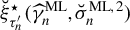 , again in dashed purple in Figure 2, however, stands out as the overall best performer in terms of RMSE and RBias when the underlying distribution is real-valued, exhibiting consistent results over all values of
$\gamma $
 . The competing GPML estimator
$\breve {\xi }_{\tau ^{\prime }_n}^{\star }(\widehat {\gamma }_n^{\mathrm {ML}},\breve {\sigma }_n^{\mathrm {ML},1})$
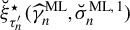 , in dashed turquoise, closely matches its top performing direct GPML counterpart only for the Student distribution with
$\gamma $
 values
$0.35$
 and
$0.4$
 , while the indirect and third direct GPML estimators
$\check {\xi }_{\tau ^{\prime }_n}^{\star }(\widehat {\gamma }_n^{\mathrm {ML}},\widehat {\sigma }_n^{\mathrm {ML}})$
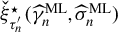 and
$\breve {\xi }_{\tau ^{\prime }_n}^{\star }(\widehat {\gamma }_n^{\mathrm {ML}},\breve {\sigma }_n^{\mathrm {ML},3})$
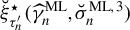 , in dash-dotted green and dashed magenta, respectively, seem to be best for the Student distribution with
$\gamma $
 values
$0.25$
 and
$0.3$
 . The indirect Moment estimator
$\check {\xi }_{\tau ^{\prime }_n}^{\star }(\widehat {\gamma }_n^{\mathrm {Mom}},\widehat {\sigma }_n^{\mathrm {Mom}})$
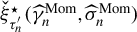 and third direct Moment estimator
$\breve {\xi }_{\tau ^{\prime }_n}^{\star }(\widehat {\gamma }_n^{\mathrm {Mom}},\breve {\sigma }_n^{\mathrm {Mom},3})$
 , again in dash-dotted blue and dashed pink, respectively, post respectable results for both distributions, but only for
$\gamma = 0.25$
 and 0.3. These results imply that our extrapolated GPD-based estimators would be well-suited to the applications to financial risk analysis which feature real-valued profit–loss distributions with comparable tail heaviness to what we have examined in these simulation experiments.
When ignoring the asymptotic bias of our direct asymmetric least squares estimators
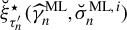
$\breve {\xi }_{\tau ^{\prime }_n}^{\star }(\widehat {\gamma }_n^{\mathrm {ML}},\breve {\sigma }_n^{\mathrm {ML},i})$
 and
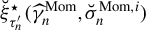
$\breve {\xi }_{\tau ^{\prime }_n}^{\star }(\widehat {\gamma }_n^{\mathrm {Mom}},\breve {\sigma }_n^{\mathrm {Mom},i})$
 for
$i=1,2,3$
 , in Corollary 1, their associated Gaussian
$100(1-\alpha )\%$
 asymptotic confidence intervals for
$\xi _{\tau ^{\prime }_n}$
 are

These confidence intervals can be calculated by using the function gpdExpect from the R package Expectrem with the respective methods "direct_ML1"
$,\ldots ,$
 "direct_ML3", and "direct_MOM1"
$,\ldots ,$
 "direct_MOM3". Likewise, under the assumption
$\lambda _1=\lambda ^{\mathrm {Mom}}=0$
 in Corollary 2, the resulting Gaussian
$100(1-\alpha )\%$
 asymptotic confidence intervals for
$\xi _{\tau ^{\prime }_n}$
 based upon the indirect quantile-based estimators
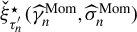
$\check {\xi }_{\tau ^{\prime }_n}^{\star }(\widehat {\gamma }_n^{\mathrm {ML}},\widehat {\sigma }_n^{\mathrm {ML}})$
 and
$\check {\xi }_{\tau ^{\prime }_n}^{\star }(\widehat {\gamma }_n^{\mathrm {Mom}},\widehat {\sigma }_n^{\mathrm {Mom}})$
 are

These confidence intervals can also be calculated by using the function gpdExpect with method="indirect_ML" and method= "indirect_MOM", respectively.
Simulation results for positive-valued distributions. Panels (a)–(d) and (e)–(h) show the coverage probabilities and average lengths, respectively, for the Fréchet distribution, while panels (i)–(l) and (m)–(p) show those for the Burr distribution. Each group of four panels is ordered by tail index value
$\gamma \in \{0.25, 0.3, 0.35, 0.4\}$
 . For
$n=1{,}500$
 and
$\tau _n' = 1 - 1/n$
 , we consider the Gaussian
$95\%$
 asymptotic confidence intervals associated with the direct BR and PS estimators
$\widehat {\xi }_{\tau ^{\prime }_n}^{\star ,\mathrm {BR}}(\widehat {\gamma }_{n}^{\mathrm {E},\mathrm {BR}})$
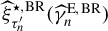 (ALS-BR) and
$\widehat {\xi }_{\tau ^{\prime }_n}^{\star ,\mathrm {PS}}$
 (ALS-PS), their indirect counterparts
$\widetilde {\xi }_{\tau ^{\prime }_n}^{\star ,\mathrm {BR}}(\widehat {\gamma }_{n}^{\mathrm {H},\mathrm {BR}})$
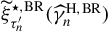 (QB-BR) and
$\widetilde {\xi }_{\tau ^{\prime }_n}^{\star ,\mathrm {PS}}$
 (QB-PS), our direct GPML estimators
$\breve {\xi }_{\tau ^{\prime }_n}^{\star }(\widehat {\gamma }_n^{\mathrm {ML}},\breve {\sigma }_n^{\mathrm {ML},1})$
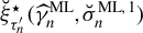 (ALS1-ML),
$\breve {\xi }_{\tau ^{\prime }_n}^{\star }(\widehat {\gamma }_n^{\mathrm {ML}},\breve {\sigma }_n^{\mathrm {ML},2})$
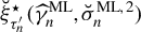 (ALS2-ML), and
$\breve {\xi }_{\tau ^{\prime }_n}^{\star }(\widehat {\gamma }_n^{\mathrm {ML}},\breve {\sigma }_n^{\mathrm {ML},3})$
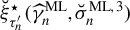 (ALS3-ML), the direct Moment estimators
$\breve {\xi }_{\tau ^{\prime }_n}^{\star }(\widehat {\gamma }_n^{\mathrm {Mom}},\breve {\sigma }_n^{\mathrm {Mom},1})$
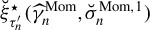 (ALS1-Mom),
$\breve {\xi }_{\tau ^{\prime }_n}^{\star }(\widehat {\gamma }_n^{\mathrm {Mom}},\breve {\sigma }_n^{\mathrm {Mom},2})$
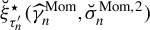 (ALS2-Mom), and
$\breve {\xi }_{\tau ^{\prime }_n}^{\star }(\widehat {\gamma }_n^{\mathrm {Mom}},\breve {\sigma }_n^{\mathrm {Mom},3})$
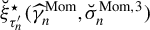 (ALS3-Mom), and the indirect GPML and Moment estimators
$\check {\xi }_{\tau ^{\prime }_n}^{\star }(\widehat {\gamma }_n^{\mathrm {ML}},\widehat {\sigma }_n^{\mathrm {ML}})$
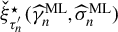 (QB-ML) and
$\check {\xi }_{\tau ^{\prime }_n}^{\star }(\widehat {\gamma }_n^{\mathrm {Mom}},\widehat {\sigma }_n^{\mathrm {Mom}})$
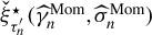 (QB-Mom).

Figure 3 Long description
The figure consists of 16 panels labeled a through p.
* Row 1 (a-d): Coverage for Frechet distribution with gamma values 0.25, 0.30, 0.35, and 0.40. The y-axis ranges from 0.00 to 1.00 with a red horizontal line at 0.95. Most curves start near 0.95 and drop sharply as k increases toward 1500.
* Row 2 (e-h): Length for Frechet distribution. The y-axis scale increases with gamma, from 0-6 in panel e to 0-15 in panel h. Curves generally show a U-shaped or decreasing trend.
* Row 3 (i-l): Coverage for Burr distribution with gamma values 0.25, 0.30, 0.35, and 0.40. Similar to row 1, curves maintain high coverage before dropping off at higher k values.
* Row 4 (m-p): Length for Burr distribution. Similar to row 2, the y-axis scale increases with gamma. Curves show varying rates of decrease and subsequent increase.
Common axes: The x-axis for all panels is k, ranging from 0 to 1500.
Legend at the bottom categorizes competitors into three groups:
1. Competitors: Q B-B R (solid orange), A L S-B R (solid light orange), Q B-P S (solid green), A L S-P S (solid light green).
2. A L S-G P D: A L S 1-M L (dashed blue), A L S 1-Mom (dashed light blue), A L S 2-M L (dashed purple), A L S 2-Mom (dashed light purple), A L S 3-M L (dashed pink), A L S 3-Mom (dashed light pink).
3. Q B-G P D: Q B-M L (dash-dot teal), Q B-Mom (dash-dot light teal).
Simulation results for real-valued distributions. Panels (a)–(d) and (e)–(h) show the coverage probabilities and average lengths, respectively, for the symmetric Burr distribution, while panels (i)–(l) and (m)–(p) show those for the Student distribution. Each group of four panels is ordered by tail index value
$\gamma \in \{0.25, 0.3, 0.35, 0.4\}$
 . For
$n=1{,}500$
 and
$\tau _n' = 1 - 1/n$
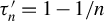 , we consider the Gaussian
$95\%$
 asymptotic confidence intervals associated with the direct BR and PS estimators
$\widehat {\xi }_{\tau ^{\prime }_n}^{\star ,\mathrm {BR}}(\widehat {\gamma }_{n}^{\mathrm {E},\mathrm {BR}})$
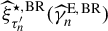 (ALS-BR) and
$\widehat {\xi }_{\tau ^{\prime }_n}^{\star ,\mathrm {PS}}$
 (ALS-PS), their indirect counterparts
$\widetilde {\xi }_{\tau ^{\prime }_n}^{\star ,\mathrm {BR}}(\widehat {\gamma }_{n}^{\mathrm {H},\mathrm {BR}})$
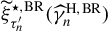 (QB-BR) and
$\widetilde {\xi }_{\tau ^{\prime }_n}^{\star ,\mathrm {PS}}$
 (QB-PS), our direct GPML estimators
$\breve {\xi }_{\tau ^{\prime }_n}^{\star }(\widehat {\gamma }_n^{\mathrm {ML}},\breve {\sigma }_n^{\mathrm {ML},1})$
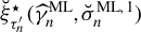 (ALS1-ML),
$\breve {\xi }_{\tau ^{\prime }_n}^{\star }(\widehat {\gamma }_n^{\mathrm {ML}},\breve {\sigma }_n^{\mathrm {ML},2})$
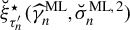 (ALS2-ML), and
$\breve {\xi }_{\tau ^{\prime }_n}^{\star }(\widehat {\gamma }_n^{\mathrm {ML}},\breve {\sigma }_n^{\mathrm {ML},3})$
 (ALS3-ML), the direct Moment estimators
$\breve {\xi }_{\tau ^{\prime }_n}^{\star }(\widehat {\gamma }_n^{\mathrm {Mom}},\breve {\sigma }_n^{\mathrm {Mom},1})$
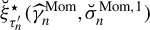 (ALS1-Mom),
$\breve {\xi }_{\tau ^{\prime }_n}^{\star }(\widehat {\gamma }_n^{\mathrm {Mom}},\breve {\sigma }_n^{\mathrm {Mom},2})$
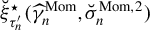 (ALS2-Mom), and
$\breve {\xi }_{\tau ^{\prime }_n}^{\star }(\widehat {\gamma }_n^{\mathrm {Mom}},\breve {\sigma }_n^{\mathrm {Mom},3})$
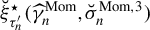 (ALS3-Mom), and the indirect GPML and Moment estimators
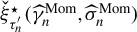
$\check {\xi }_{\tau ^{\prime }_n}^{\star }(\widehat {\gamma }_n^{\mathrm {ML}},\widehat {\sigma }_n^{\mathrm {ML}})$
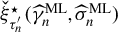 (QB-ML) and
$\check {\xi }_{\tau ^{\prime }_n}^{\star }(\widehat {\gamma }_n^{\mathrm {Mom}},\widehat {\sigma }_n^{\mathrm {Mom}})$
 (QB-Mom).

Figure 4 Long description
The figure consists of 16 line graphs arranged in a 4 by 4 grid.
Rows 1 and 2 (panels a through h) represent the symmetric Burr distribution.
- Row 1 (a-d) shows Coverage on the y-axis (0.00 to 1.00) against k on the x-axis (0 to 800). A red horizontal line marks the 0.95 target. Most estimators start near 1.00 and drop sharply as k increases, with the drop-off point shifting right as the tail index gamma increases from 0.25 to 0.40.
- Row 2 (e-h) shows Length on the y-axis (0 to 15) against k. Curves generally show a U-shape or a steady decline followed by a sharp rise at high k values.
Rows 3 and 4 (panels i through p) represent the Student distribution.
- Row 3 (i-l) shows Coverage. Similar to the Burr distribution, coverage stays near 0.95 for low k and drops toward 0.00. The A L S-P S and A L S-B R estimators (solid green and orange lines) drop much earlier than the Q B and A L S-M L variants (dashed lines).
- Row 4 (m-p) shows Length. The curves exhibit a downward trend as k increases, with higher tail index values resulting in higher initial length values on the y-axis.
The legend at the bottom categorizes competitors into three groups:
1. Competitors: Q B-B R, A L S-B R, Q B-P S, and A L S-P S (solid lines).
2. A L S-G P D: A L S 1-M L, A L S 1-Mom, A L S 2-M L, A L S 2-Mom, A L S 3-M L, and A L S 3-Mom (dashed lines in blue, purple, and pink).
3. Q B-G P D: Q B-M L and Q B-Mom (dotted-dashed lines in teal).
We plot the coverage probabilities and average lengths of the
$95\%$
 confidence intervals against k for the positive and real-valued distributions in Figures 3 and 4, respectively. While most confidence intervals associated with the 12 competing extrapolated estimators are able to get close to the intended
$95\%$
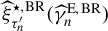
 coverage as k varies, very few can achieve that for a wide range of k values. Our direct GPML confidence intervals
$\breve {I}_{\tau ^{\prime }_n}^{\mathrm {ML},i}$
 , and particularly those associated with the estimators
$\breve {\xi }_{\tau ^{\prime }_n}^{\star }(\widehat {\gamma }_n^{\mathrm {ML}},\breve {\sigma }_n^{\mathrm {ML},1})$
 and
$\breve {\xi }_{\tau ^{\prime }_n}^{\star }(\widehat {\gamma }_n^{\mathrm {ML}},\breve {\sigma }_n^{\mathrm {ML},2})$
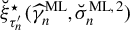 with coverage probabilities in dashed turquoise and dashed purple, respectively, achieve coverage levels that are reasonably close to the nominal level for both the positive and real-valued distributions, and for all studied values of
$\gamma $
 ; it should here be taken into account that, unlike the estimators
$\widehat {\xi }_{\tau ^{\prime }_n}^{\star ,\mathrm {BR}}(\widehat {\gamma }_{n}^{\mathrm {E},\mathrm {BR}})$
 and
$\widetilde {\xi }_{\tau ^{\prime }_n}^{\star ,\mathrm {BR}}(\widehat {\gamma }_{n}^{\mathrm {H},\mathrm {BR}})$
 , the proposed GPML intervals do not benefit from extensive finite-sample corrections. And while these estimators fall short of the indirect bias-reduced
$\widetilde {\xi }_{\tau ^{\prime }_n}^{\star ,\mathrm {BR}}(\widehat {\gamma }_{n}^{\mathrm {H},\mathrm {BR}})$
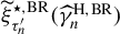 estimator’s tight interval lengths, they still post respectable results, especially around the higher k values where they record their most competitive RMSE and RBias in Figures 1 and 2. The larger average lengths of our confidence intervals can be attributed to the additional uncertainty that our estimation and inference procedures must account for, as they incorporate estimates of the location, scale, and shape parameters of the GP distribution, whereas the Weissman-type competitors are constructed on scale and shape parameter estimates only. Another notable outlier is the second direct Moment estimator
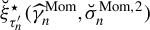
$\breve {\xi }_{\tau ^{\prime }_n}^{\star }(\widehat {\gamma }_n^{\mathrm {Mom}},\breve {\sigma }_n^{\mathrm {Mom},2})$
 as it shows encouraging coverage, in dashed mauve, for all cases of the symmetric Burr distribution, as well as Student cases with
$\gamma = 0.35$
 and
$0.4$
 .
Finally, it should be noted that our experience with simulated data indicates that the chosen asymptotic confidence intervals
$\breve {I}_{\tau ^{\prime }_n}^{\mathrm {ML},i}$
 ,
$\breve {I}_{\tau ^{\prime }_n}^{\mathrm {Mom},i}$
 ,
$\check {I}_{\tau ^{\prime }_n}^{\mathrm {ML}}$
 , and
$\check {I}_{\tau ^{\prime }_n}^{\mathrm {Mom}}$
 , obtained from the asymptotics in Theorems 1 and 3, afford better results (for both nonnegative and real-valued distributions) than their respective counterparts that are derived from the equivalent convergences in (2.8) and (2.11), mainly due to the reliance of the former confidence intervals on additional location parameter estimates. This is illustrated for the positive and real-valued distributions in Figures 5 and 6, respectively, where we visualize the dominance of the chosen direct GPML confidence intervals
$\breve {I}_{\tau ^{\prime }_n}^{\mathrm {ML},1}$
 and
$\breve {I}_{\tau ^{\prime }_n}^{\mathrm {ML},2}$
 , in terms of both coverage probabilities and average lengths, over their alternate confidence intervals that are constructed from the convergence (2.8).
Simulation results for positive-valued distributions. Panels (a)–(d) and (e)–(h) show the coverage probabilities and average lengths, respectively, for the Fréchet distribution, while panels (i)–(l) and (m)–(p) show those for the Burr distribution. Each group of four panels is ordered by tail index value
$\gamma \in \{0.25, 0.3, 0.35, 0.4\}$
 . For
$n=1{,}500$
 and
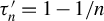
$\tau _n' = 1 - 1/n$
 , we consider the chosen direct GPML confidence intervals
$\breve {I}_{\tau ^{\prime }_n}^{\mathrm {ML},1}$
 and
$\breve {I}_{\tau ^{\prime }_n}^{\mathrm {ML},2}$
 (solid lines), constructed from the convergence in Theorem 1, and their alternate counterparts (dashed lines) that are constructed from the equivalent convergence (2.8).

Figure 5 Long description
The 16 panels are labeled a through p.
* Row 1 (a-d): Coverage for Frechet distribution. The x-axis is k from 0 to 1500, and the y-axis is Coverage from 0.00 to 1.00. A red horizontal line marks the 0.95 threshold. Solid and dashed lines for A L S 1-M L and A L S 2-M L stay near 0.95 for low k but drop sharply toward zero as k exceeds 1000, with A L S 1-M L (teal) dropping earlier than A L S 2-M L (purple).
* Row 2 (e-h): Length for Frechet distribution. The y-axis scale increases with gamma, from 0-6 in panel e to 0-15 in panel h. All lines show a sharp initial peak followed by a gradual asymptotic decay as k increases. Dashed lines (Alternate C I) maintain higher values than solid lines (Chosen C I).
* Row 3 (i-l): Coverage for Burr distribution. Similar to Row 1, coverage is stable near 0.95 for small k. The teal lines (A L S 1-M L) show a significant dip and partial recovery or stabilization around k equals 1250, while purple lines (A L S 2-M L) remain more stable.
* Row 4 (m-p): Length for Burr distribution. Trends mirror Row 2, showing a sharp peak at very low k followed by a downward curve. The vertical scale again increases with the tail index gamma.
Legend at the bottom: Alternate C I is represented by dashed lines (teal for A L S 1-M L, purple for A L S 2-M L). Chosen C I is represented by solid lines (teal for A L S 1-M L, purple for A L S 2-M L).
Simulation results for real-valued distributions. Panels (a)–(d) and (e)–(h) show the coverage probabilities and average lengths, respectively, for the symmetric Burr distribution, while panels (i)–(l) and (m)–(p) show those for the Student distribution. Each group of four panels is ordered by tail index value
$\gamma \in \{0.25, 0.3, 0.35, 0.4\}$
 . For
$n=1{,}500$
 and
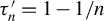
$\tau _n' = 1 - 1/n$
 , we consider the chosen direct GPML confidence intervals
$\breve {I}_{\tau ^{\prime }_n}^{\mathrm {ML},1}$
 and
$\breve {I}_{\tau ^{\prime }_n}^{\mathrm {ML},2}$
 (solid lines), constructed from the convergence in Theorem 1, and their alternate counterparts (dashed lines) that are constructed from the equivalent convergence (2.8).

Figure 6 Long description
The figure consists of 16 panels labeled a through p.
* Panels a through d (Top Row): Coverage for symmetric Burr distribution. The y-axis ranges from 0.00 to 1.00. A red horizontal line marks the 0.95 threshold. Solid and dashed lines for A L S 1 M L and A L S 2 M L show varying stability, with A L S 1 M L (teal) showing a significant dip in coverage as k increases beyond 400 in panel a, which becomes less pronounced as the tail index increases to 0.40 in panel d.
* Panels e through h (Second Row): Average length for symmetric Burr distribution. The y-axis scale increases with the tail index, from 0 to 6 in panel e up to 0 to 15 in panel h. All curves show an initial sharp peak followed by a gradual decline. Dashed lines (Alternate C I) remain consistently higher than solid lines (Chosen C I).
* Panels i through l (Third Row): Coverage for Student distribution. These panels show much higher stability than the symmetric Burr plots, with most lines remaining near the 0.95 red line across the entire range of k, though a slight downward trend is visible in the solid lines as k approaches 800.
* Panels m through p (Bottom Row): Average length for Student distribution. Similar to the symmetric Burr length plots, these show a sharp initial rise and a smooth asymptotic decay. The A L S 1 M L and A L S 2 M L lines are nearly overlapping for the Chosen C I (solid lines), while the Alternate C I (dashed lines) are significantly higher.
Legend at the bottom indicates:
* Alternate C I: Dashed teal line for A L S 1 M L and dashed purple line for A L S 2 M L.
* Chosen C I: Solid teal line for A L S 1 M L and solid purple line for A L S 2 M L.
4 APPLICATION TO DYNAMIC TAIL RISK FORECASTING
We apply our extreme expectile estimation methodologies to evaluate tail risk for the stocks of Netflix, Walmart, and American Express, as well as the exchange rate of Bitcoin (BTC-USD). Our goal is to forecast the expectile risk measure of tomorrow given the knowledge of today. To this end, we adopt a rolling window approach to our analysis, with each window size set to
$n = 1{,}500$
 , and utilize data on the daily loss returns (i.e., negative log-returns)
$Y_1,\ldots ,Y_n$
 of the aforementioned stocks and exchange rate. Using this setup and a careful selection of observation dates, we arrive at the following data specifications:
-
• Netflix: 498 estimation windows between $2008/12/03$
and
$2016/11/08$
. -
• Walmart: 482 windows between $2013/11/13$
and
$2021/09/28$
. -
• American Express: 766 windows between $2011/11/16$
and
$2020/11/17$
. -
• Bitcoin-USD: 217 windows between $2016/04/28$
and
$2021/01/08$
.








We follow the strategy laid out in Girard et al. (Reference Girard, Stupfler and Usseglio-Carleve2022b) of filtering our time series through the lens of an ARMA(1,1)-GARCH(1,1) model. For a rolling window
$Y_1, \ldots , Y_n$
 , we set up the model
$ Y_t = \mu + \phi Y_{t-1} + u_t + \theta u_{t-1}, $
 where
$u_t = \sigma _t \varepsilon _t$
 such that
$\sigma _t^2 = c + au_{t-1}^2 + b\sigma _{t-1}^2$
 and
$\left (\varepsilon _t\right )$
 is an unobserved independent white noise sequence, while the constants
$\mu , \phi , \theta , a, b,$
 and c are model parameters. Using the positive homogeneity and location equivariance of expectiles, we can then write the conditional
$\tau $
 th expectile for the next day as

where
$\mathcal {F}_n$
 is the
$\sigma $
 -algebra generated by the ARMA-GARCH process up to time n.
We first estimate the ARMA-GARCH model parameters using the function garchFit in the R package fGarch, which allows us to retrieve the raw residuals
$\widehat {u}_i$
 through the @residuals option. Following the ideas of Girard et al. (Reference Girard, Stupfler and Usseglio-Carleve2022b), we then fit a GARCH(1,1) model to
$\widehat {u}_i$
 and retrieve the predictions
$\widehat {\varepsilon }_i$
 of the innovations from the GARCH residuals. These filtered residuals can then be considered as independent and identically distributed copies of
$\varepsilon $
 , which facilitates the estimation procedures laid out in this work. The extrapolated extreme expectile estimates

for
$i \in \{1,2,3\}$
 , paired with estimates of the ARMA-GARCH model parameters
$\widehat {\mu }$
 ,
$\widehat {\phi }$
 ,
$\widehat {\theta }$
 ,
$\widehat {a}$
 ,
$\widehat {b}$
 , and
$\widehat {c}$
 , can be combined to construct the dynamic predictions of the extreme expectiles of
$Y_{n+1}$
 given
$Y_n$
 as

Recall that a functional T is elicitable relative to a class of distributions
$\mathcal {F}$
 if there exists a scoring function
$S:\mathbb {R}\times \mathbb {R}\to \mathbb {R}$
 such that
$\mathbb {E}_F\{S(t,Y)\}\leq \mathbb {E}_F\{S(x,Y)\}$
 for every
$F\in \mathcal {F}$
 , every
$t\in T(F)$
 , and every
$x\in \mathbb {R}$
 , with equality if and only if
$x\in T(F)$
 (Gneiting, Reference Gneiting2011, Def. 2). This property provides a natural basis for evaluating and comparing the 12 competing forecasters. For the expectile at level
$\tau _n'$
 , we use the asymmetric least squares scoring function
$ L_{\tau _n'}: \, \mathbb {R}^2 \to [0,\infty ), \, (\xi ,y)\mapsto | \tau _n'-\mathbb {1} \{ y\leq \xi \}| (y-\xi )^2 $
 , which gives the loss
$L_{\tau _n'}(\xi ,y)$
 when the point forecast
$\xi $
 is issued and the realization y of the future observation materializes. Following Ziegel (Reference Ziegel2016), given T forecast cases with point forecasts
$(\xi ^{(m)}_1,\ldots ,\xi ^{(m)}_T)$
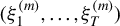 and realizing observations
$(y_1,\ldots ,y_T)$
 , where the index m numbers the competing forecasters, the latter can be ranked in terms of their average realized loss (the lower the better)

where each forecast case
$t\in \{1,\ldots ,T\}$
 corresponds in our estimation context to a rolling window of loss returns
$Y_1, \ldots , Y_n$
 , with
$y_t$
 representing the realization of the future observation
$Y_{n+1}$
 , and
$\xi ^{(m)}_t$
 being its point forecast
$\overline {\xi }_{\tau _n'}(Y_{n+1}|\mathcal {F}_n)$
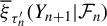 obtained in (4.2) from the 12 competitors
$\overline {\xi }_{\tau _n'} (\varepsilon )$
 in (4.1). In our assessment of tail risk, we compare the average scores
$\mathcal {L}^{(m)}_{\tau _n'}$
 for a fine grid of challenging levels
$\tau _n' \in \{0.99, \ldots , 1-1/n\}$
 , where data are sparse and inference is difficult to handle. To guide our choice of the intermediate sequence
$k_n$
 , which plays the role of the tuning parameter in our setup, we calculate the average realized loss for every value k in the range of all possible values of
$k_n$
 , then select the value that yields the lowest loss for each estimator and each value of
$\tau _n'$
 . This approach simplifies the optimal
$k_n$
 selection process while allowing us to compare the performance of each forecaster fairly. Figures 7–10 show the results of our analysis of daily loss returns of Netflix, Walmart, American Express, and Bitcoin-USD, respectively.
Netflix data. (A) Observed negative log returns, with realizations wrapped between dashed red lines. (B) KPSS test statistic of stationarity (in blue) with the
$5\%$
 critical value in dotted gray, both against the rolling window index. (C) p-values of the Ljung–Box test of independence, with 30 lags, for the residuals
$\widehat {\varepsilon }_i$
 and their squares
$\widehat {\varepsilon }^2_i$
 against the rolling window index. (D) Collage of
$\widehat {\gamma }_n^{\mathrm {ML}}$
 and
$\widehat {\gamma }_n^{\mathrm {Mom}}$
 against k; each curve corresponds to a distinct rolling window. (E) Comparison of the competing estimators on the basis of realized loss
$\mathcal {L}^{(m)}_{\tau _n'}$
 for
$\tau _n' \in \{0.99, \ldots , 1-1/n\}$
 and
$m=1,\ldots ,12$
 . (F) Next-day forecasts (black curve)
$\breve {\xi }_{\tau ^{\prime }_n}^{\star }(\widehat {\gamma }_n^{\mathrm {Mom}},\breve {\sigma }_n^{\mathrm {Mom},1})$
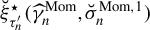 of
$\xi _{\tau ^{\prime }_n}$
 at level
$\tau _n' = 0.99$
 , for the daily loss returns computed sequentially over each rolling window, with
$95\%$
 lower (blue curve) and upper (magenta curve) asymptotic confidence bounds, along with the realization of the future observation (gray curve).

Figure 7 Long description
Panel A is a line graph of Daily Loss Return against Date from 2008/12/03 to 2016/11/08. The data fluctuates around zero with two vertical dashed red lines marking a specific period. Panel B shows the K P S S test statistic as a blue line against a rolling window index. The line remains well below a dotted gray horizontal line representing the 5 percent critical value. Panel C displays P-values for the Ljung-Box test. A blue line for residuals and a magenta line for squared residuals both stay above a dotted gray line at 0.05. Panel D shows E V I estimates against k. It features a dense collage of cyan curves for G P M L and magenta curves for Moment estimators, both showing a sharp initial peak followed by a gradual decline. Panel E compares realized loss against target level from 0.990 to 1 - 1/1500 (approximately 0.999333). Multiple downward-sloping curves are shown, with solid lines for Q B and A L S estimators and dashed lines for A L S 1, A L S 2, and A L S 3 variants. Panel F shows next-day forecasts. A black line for forecasts is centered between a magenta dashed upper bound and a blue dashed lower bound, all overlaid on a light gray line representing actual realizations of daily loss returns.
Walmart data. (A) Observed negative log returns, with realizations wrapped between dashed red lines. (B) KPSS test statistic of stationarity (in blue) with the
$5\%$
 critical value in dotted gray, both against the rolling window index. (C) p-values of the Ljung–Box test of independence, with 30 lags, for the residuals
$\widehat {\varepsilon }_i$
 and their squares
$\widehat {\varepsilon }^2_i$
 against the rolling window index. (D) Collage of
$\widehat {\gamma }_n^{\mathrm {ML}}$
 and
$\widehat {\gamma }_n^{\mathrm {Mom}}$
 against k; each curve corresponds to a distinct rolling window. (E) Comparison of the competing estimators on the basis of realized loss
$\mathcal {L}^{(m)}_{\tau _n'}$
 for
$\tau _n' \in \{0.99, \ldots , 1-1/n\}$
 and
$m=1,\ldots ,12$
 . (F) Next-day forecasts (black curve)
$\breve {\xi }_{\tau ^{\prime }_n}^{\star }(\widehat {\gamma }_n^{\mathrm {Mom}},\breve {\sigma }_n^{\mathrm {Mom},1})$
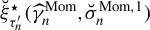 of
$\xi _{\tau ^{\prime }_n}$
 at level
$\tau _n' = 0.99$
 , for the daily loss returns computed sequentially over each rolling window, with
$95\%$
 lower (blue curve) and upper (magenta curve) asymptotic confidence bounds, along with the realization of the future observation (gray curve).

Figure 8 Long description
The figure consists of six line graphs arranged in a two-by-three grid.
Panel A, Walmart Daily Loss Return: A time series plot from 2013/11/13 to 2021/09/28. The data fluctuates around zero with several sharp downward spikes. Two vertical dashed red lines mark a specific period around 2020.
Panel B, K P S S test of stationarity: The y-axis is the Test Statistic and the x-axis is the Rolling window. A blue line fluctuates between 0.0 and 0.4, staying below a dotted gray horizontal line representing the 5 percent critical value.
Panel C, Ljung-Box test of independence: The y-axis is the P-Value and the x-axis is the Rolling window. A blue line for residuals and a magenta line for squared residuals both stay well above a dotted gray line at 0.05.
Panel D, E V I Estimates: The y-axis is E V I and the x-axis is k. It shows a dense collage of cyan G P M L curves and magenta Moment curves. The curves generally converge and trend downward as k increases beyond 100.
Panel E, Forecast Comparison: The y-axis is Realized Loss and the x-axis is Target Level from 0.990 to 1 - 1/1500 (approximately 0.999333). Multiple colored lines, including Q B and A L S variants, show a consistent downward slope as the target level increases.
Panel F, Top Ranked Forecaster: A time series plot from 2020 to 2021. A black forecast line follows a gray realization line. Magenta and blue dashed lines represent the 95 percent upper and lower confidence bounds, which widen during periods of high volatility.
American Express data. (A) Observed negative log returns, with realizations wrapped between dashed red lines. (B) KPSS test statistic of stationarity (in blue) with the
$5\%$
 critical value in dotted gray, both against the rolling window index. (C) p-values of the Ljung–Box test of independence, with 30 lags, for the residuals
$\widehat {\varepsilon }_i$
 and their squares
$\widehat {\varepsilon }^2_i$
 against the rolling window index. (D) Collage of
$\widehat {\gamma }_n^{\mathrm {ML}}$
 and
$\widehat {\gamma }_n^{\mathrm {Mom}}$
 against k; each curve corresponds to a distinct rolling window. (E) Comparison of the competing estimators on the basis of realized loss
$\mathcal {L}^{(m)}_{\tau _n'}$
 for
$\tau _n' \in \{0.99, \ldots , 1-1/n\}$
 and
$m=1,\ldots ,12$
 . (F) Next-day forecasts (black curve)
$\check {\xi }^\star _{\tau ^{\prime }_n}(\widehat {\gamma }_n^{\mathrm {Mom}},\widehat {\sigma }_n^{\mathrm {Mom}})$
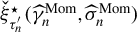 at level
$\tau _n' = 0.99$
 , for the daily loss returns computed sequentially over each rolling window, with
$95\%$
 lower (blue curve) and upper (magenta curve) asymptotic confidence bounds, along with the realization of the future observation (gray curve).

Figure 9 Long description
Panel A is a line graph of Daily Loss Return from 2011/11/16 to 2020/11/17. The data fluctuates around zero with a significant spike in volatility around 2020, marked by two vertical dashed red lines.
Panel B shows the K P S S test statistic against the rolling window index. A blue line fluctuates between 0.0 and 0.4, remaining below a dotted gray critical value line at approximately 0.46.
Panel C displays p-values for the Ljung-Box test. A blue line represents residuals and a purple line represents squared residuals. Both fluctuate significantly above a 0.05 dashed threshold, with the purple line staying closer to 1.0.
Panel D shows E V I estimates against k. It contains a dense collage of cyan curves for G P M L and magenta curves for Moment estimators, both converging as k increases toward 500.
Panel E is a forecast comparison showing realized loss against target level from 0.990 to 0.998. Multiple colored dashed and solid lines show a consistent downward linear trend as the target level increases.
Panel F shows the top-ranked forecaster Q B-Mom. A black forecast line follows the upper peaks of a gray realization line. Magenta and blue dashed lines represent the 95 percent upper and lower confidence bounds, which widen during the high-volatility period in 2020.
Bitcoin-USD data. (A) Observed negative log returns, with realizations wrapped between dashed red lines. (B) KPSS test statistic of stationarity (in blue) with the
$5\%$
 critical value in dotted gray, both against the rolling window index. (C) p-values of the Ljung–Box test of independence, with 30 lags, for the residuals
$\widehat {\varepsilon }_i$
 and their squares
$\widehat {\varepsilon }^2_i$
 against the rolling window index. (D) Collage of
$\widehat {\gamma }_n^{\mathrm {ML}}$
 and
$\widehat {\gamma }_n^{\mathrm {Mom}}$
 against k; each curve corresponds to a distinct rolling window. (E) Comparison of the competing estimators on the basis of realized loss
$\mathcal {L}^{(m)}_{\tau _n'}$
 for
$\tau _n' \in \{0.99, \ldots , 1-1/n\}$
 and
$m=1,\ldots ,12$
 . (F) Next-day forecasts (black curve)
$\breve {\xi }_{\tau ^{\prime }_n}^{\star }(\widehat {\gamma }_n^{\mathrm {Mom}},\breve {\sigma }_n^{\mathrm {Mom},1})$
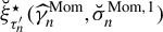 of
$\xi _{\tau ^{\prime }_n}$
 at level
$\tau _n' = 0.99$
 , for the daily loss returns computed sequentially over each rolling window, with
$95\%$
 lower (blue curve) and upper (magenta curve) asymptotic confidence bounds, along with the realization of the future observation (gray curve).

Figure 10 Long description
Panel A shows a time series of daily loss returns from 2016/04/28 to 2021/01/08, characterized by high volatility and a significant spike in early 2020. Two vertical dashed red lines mark a specific realization window near the end of the series.
Panel B displays the K P S S test statistic as a solid blue line against a rolling window index. The line fluctuates between 0.2 and 0.35, remaining well below the dotted gray 5 percent critical value line at approximately 0.46.
Panel C plots P-values for the Ljung-Box test. Residuals squared are shown as a constant magenta line at 1.0. Residuals are shown as a fluctuating blue line mostly above the 0.05 significance threshold, with occasional dips toward it.
Panel D shows E V I estimates against k. The G P M L estimator in cyan and the Moment estimator in magenta both show high variance for low k, with the Moment estimator trending upward and the G P M L estimator stabilizing around 0.15 as k increases.
Panel E compares realized loss across target levels from 0.990 to 1 - 1/1500 (approximately 0.999333). Multiple curves representing different estimators, including Q B, A L S, M L, and Mom, show a consistent downward trend as the target level increases.
Panel F presents next-day forecasts. A black forecast line follows the general trend of the gray realization line. Magenta and blue dashed lines represent the 95 percent upper and lower asymptotic confidence bounds, respectively, for the estimated extreme expectile.
In each figure, Panel (A) showcases the observed data and wraps the realizations
$y_t$
 between two dashed red lines. Panel (B) shows the results of the Kwiatkowski–Phillips–Schmidt–Shin (KPSS) test for each rolling window, illustrating the stationarity of our loss returns over all chosen time periods, which is required for ARMA-GARCH modeling. Panel (C) then examines the independence of the residuals
$\widehat {\varepsilon }_i$
 using a Ljung–Box test on these residuals and their squares. This independence is a prerequisite for conducting inference on extreme expectiles from our Corollaries 1 and 2 and the asymptotic theory of the Weissman-type competitors. The residuals’ tail heaviness is evaluated in Panel (D) through a study of the GPML (
$\widehat {\gamma }_n^{\mathrm {ML}}$
 ) and Moment (
$\widehat {\gamma }_n^{\mathrm {Mom}}$
 ) estimates of the EVI against an appropriate range of possible values k of the intermediate level
$k_n$
 . The results from each rolling window are drawn as an individual curve against k and indicate that the residuals exhibit consistent tail heaviness over all estimation windows for a wide range of k values. Panel (E) then displays the average realized loss
$\mathcal {L}^{(m)}_{\tau _n'}$
 , defined in (4.3), for each estimator against
$\tau _n'$
 , using the optimal
$k_n$
 value that minimizes said loss. The good news for practitioners concerned with the accuracy of daily forecasts is that our GPD-based forecasters outperform all Weissman-type competitors, for each studied financial time series. More specifically, the direct Moment estimator
$\breve {\xi }_{\tau ^{\prime }_n}^{\star }(\widehat {\gamma }_n^{\mathrm {Mom}},\breve {\sigma }_n^{\mathrm {Mom},1})$
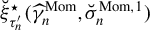 establishes a clear lead for Netflix, Walmart, and Bitcoin-USD data, with estimators like the second direct Moment estimator
$\breve {\xi }_{\tau ^{\prime }_n}^{\star }(\widehat {\gamma }_n^{\mathrm {Mom}},\breve {\sigma }_n^{\mathrm {Mom},2})$
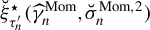 , the third direct Moment estimator
$\breve {\xi }_{\tau ^{\prime }_n}^{\star }(\widehat {\gamma }_n^{\mathrm {Mom}},\breve {\sigma }_n^{\mathrm {Mom},3}),$
 and the indirect Moment estimator
$\check {\xi }^\star _{\tau ^{\prime }_n}(\widehat {\gamma }_n^{\mathrm {Mom}},\widehat {\sigma }_n^{\mathrm {Mom}})$
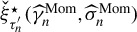 trailing close behind. The American Express data see the indirect Moment estimator
$\check {\xi }^\star _{\tau ^{\prime }_n}(\widehat {\gamma }_n^{\mathrm {Mom}},\widehat {\sigma }_n^{\mathrm {Mom}})$
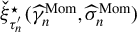 , respectively, the direct GPML estimator
$\breve {\xi }_{\tau ^{\prime }_n}^{\star }(\widehat {\gamma }_n^{\mathrm {ML}},\breve {\sigma }_n^{\mathrm {ML},2})$
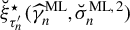 , outperform all of the Weissman competitors for
$\tau _n'< 0.995$
 , respectively,
$\tau _n'\geq 0.995$
 . The results imply that our Moment- and GPML-based estimators are suitable for financial data, which corroborates our simulation findings in Section 3, where said estimators scored ahead of the competition in the case of real-valued distributions. The final panel (F) wraps up by showing next-day forecasts of
$\xi _{\tau ^{\prime }_n}$
 at level
$\tau _n' = 0.99$
 , for the daily loss returns over the observation period, using the dynamic predictions (4.2) of the top-ranked forecaster
$\breve {\xi }_{\tau ^{\prime }_n}^{\star }(\widehat {\gamma }_n^{\mathrm {Mom}},\breve {\sigma }_n^{\mathrm {Mom},1})$
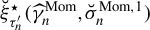 for Netflix, Walmart, and Bitcoin-USD, and
$\check {\xi }^\star _{\tau ^{\prime }_n}(\widehat {\gamma }_n^{\mathrm {Mom}},\widehat {\sigma }_n^{\mathrm {Mom}})$
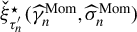 for American Express, along with their
$95\%$
 asymptotic confidence intervals and the realization of the future observation. The point forecasts and associated confidence bounds seem to follow data trends fairly closely.
5 DISCUSSION
Tail expectiles define a prime candidate for a standard risk measure in finance and insurance thanks to their excellent axiomatic properties and their ability to capture essential information about the severity of extreme observations as well as their probabilities. The problem of correctly estimating and inferring extreme expectile risk is a difficult question due to the least squares nature of expectiles and their sensitivity to tail heaviness, even though a series of recent papers has focused on this problem using Weissman-type extrapolation devices. Our Generalized Pareto approach provides good estimates of tail risk across the board, with reasonably accurate (though elementary) asymptotic Gaussian confidence intervals, in the financial context of heavy-tailed real-valued profit–loss distributions without resorting to any bias correction of our estimators, even though their asymptotic behavior indicates that they are asymptotically biased. The results of the tail risk forecasting exercise we have carried out similarly indicate that, in a dynamic estimation setting, the Generalized Pareto extrapolation method yields encouraging results.
There still remains a lot to be done, especially in the actuarial context of nonnegative heavy-tailed loss variables for which Weissman-type methods seem to outperform our GPD-based approach. As we have highlighted, asymptotic Gaussian inference of extreme expectiles may not perform well in finite samples, because of the difficulty of tracking the statistical uncertainties of the estimated high expectiles and the use of the asymptotic variances arising in the Gaussian limiting distributions. The finite-sample approximations and errors thus made are typically due to (i) the use of the GPD model when no parametric assumption about the exceedance distribution is desired, (ii) the asymptotic approximations motivating the extreme value estimators of the scale and shape parameters, (iii) the use of the asymptotic connection between extreme expectiles and quantiles while ignoring higher-order error terms, (iv) incorrectly neglecting correlations between estimators when the asymptotic behavior of one of them dominates, and/or (v) not accounting for the variance distortions incurred by utilizing the delta method for linearization purposes. Improving our results by providing successive corrections for each of these types of approximation errors is a topic of interest for future research.
APPENDIXES
The Appendix has three parts. Appendix A presents an overview of the current state of research on tail expectile estimation. Appendix B provides further details about bias reduction and variance correction within the Weissman extrapolation framework. Appendix C contains the proofs of all theoretical results in the main article.
A WEISSMAN-TYPE ESTIMATORS
Let
$X_1, \ldots , X_n$
 be a sample of observations drawn from F, and for the moment assume that these random copies of X are independent. Let
$X_{1,n}\leqslant \cdots \leqslant X_{n,n}$
 be their corresponding order statistics. In the intermediate case when
$\tau = \tau _n \to 1$
 such that
$n(1-\tau _n)\to \infty $
 as
$n \to \infty $
 , or under the more common discretized setup
$\tau _n =1-k/n $
 for a sequence of integers
$k=k_n\to \infty $
 with
$k_n/n \to 0$
 as
$n \to \infty $
 , the population expectile
$\xi _{\tau _n}$
 is extreme but well inside the sample so that it can be consistently estimated by its empirical version

where
$\eta _{\tau }(y)=|\tau -\mathbb {1} \{ y\leqslant 0 \}|y^2$
 . The asymptotic normality of
$\widehat {\xi }_{\tau _n}$
 is derived in Theorem 2 in Daouia et al. (Reference Daouia, Girard and Stupfler2018) for the class of heavy-tailed distributions (2.2) with
$\gamma <1/2$
 . In the more general setting where
$0<\gamma <1$
 , an indirect asymptotically normal estimator of
$\xi _{\tau _n}$
 can be obtained from the asymptotic connection (2.5), or equivalently,
$ \xi _{\tau _n}\sim (\gamma ^{-1}-1)^{-\gamma }{q_{\tau _n}} \text { as } n\to \infty. $
 By substituting in a suitable estimator
$\overline {\gamma }$
 in place of
$\gamma $
 and the empirical quantile
$\widehat {q}_{\tau _n}= X_{n-\lfloor n(1-\tau _n) \rfloor ,n}=X_{n-k,n}$
 in place of
$q_{\tau _n}$
 , the resulting estimator

is shown to have a
$\sqrt {n(1-\tau _n)}$
 -asymptotic nondegenerate distribution under the conditions formulated in Theorem 1 in Daouia et al. (Reference Daouia, Girard and Stupfler2018). The EVI
$\gamma \in (0,1)$
 can be estimated by the celebrated Hill estimator (Hill, Reference Hill1975)
$\widehat {\gamma }_{n}^{\mathrm {H}}:= \frac {1}{\lfloor n(1-\tau _n) \rfloor } \sum _{i=1}^{\lfloor n(1-\tau _n) \rfloor } \log X_{n-i+1,n}-\log X_{n-\lfloor n(1-\tau _n) \rfloor ,n}, $
 or, in the case
$\gamma \in (0,1/2)$
 , by the following expectile-based estimator introduced and popularized by Girard et al. (Reference Girard, Stupfler and Usseglio-Carleve2022a, Reference Girard, Stupfler and Usseglio-Carleve2022b):

In the more challenging extreme case when
$\tau = \tau ^{\prime }_n \to 1$
 such that
$n(1-\tau ^{\prime }_n)\to c\in [0,\infty )$
 as
$n \to \infty $
 , the population expectile
$\xi _{\tau ^{\prime }_n}$
 lies at the far tail of the underlying distribution, possibly beyond the sample maximum
$X_{n,n}$
 in the data. Typical examples include
$\tau ^{\prime }_n=1-1/n$
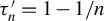 , with the associated extreme expectile
$\xi _{\tau ^{\prime }_n}$
 having the order of magnitude of
$X_{n,n}$
 . In this case, the model assumption of Pareto-type tail (2.2), combined with the asymptotic connection (2.5), yields the Weissman approximation

This approximation motivates the following class of plug-in estimators of
$\xi _{\tau ^{\prime }_n}:$


where
$\overline {\gamma }$
 is a
$\sqrt {n(1-\tau _{n})}$
 -consistent estimator of
${\gamma }$
 , and
$\overline {\xi }_{\tau _n}$
 is either the empirical asymmetric least squares estimator
$\widehat {\xi }_{\tau _n}$
 in (A.1) or the quantile-based estimator
$\widetilde {\xi }_{\tau _n}$
 in (A.2) for the intermediate expectile
$\xi _{\tau _n}.$
 More specifically, the use of the latter indirect intermediate expectile
$\overline {\xi }_{\tau _n}\equiv \widetilde {\xi }_{\tau _n}$
 in (A.5) yields the extreme expectile estimator
$\widetilde {\xi }^\star _{\tau ^{\prime }_n}:=\overline {\xi }^\star _{\tau ^{\prime }_n}$
 defined as

while the choice of the former direct intermediate expectile
$\overline {\xi }_{\tau _n}\equiv \widehat {\xi }_{\tau _n}$
 results in

Based on an i.i.d. assumption on the sample and an SORV condition
$\mathcal {C}_2(\gamma , \tilde {\rho }, \tilde {A})$
 with additional mild regularity conditions, Daouia et al. (Reference Daouia, Girard and Stupfler2018) have shown in their Corollaries 3 and 4 that the estimators (A.6) and (A.7) have the same limit distribution as the chosen tail index estimator
$\overline {\gamma }$
 with the slightly slower rate of convergence
$\log ((1-\tau _n)/(1-\tau ^{\prime }_n))/\sqrt {n(1-\tau _n)}$
 . In the rest of this Appendix, for the sake of notational convenience, we set
$\rho =\tilde {\rho }$
 and
$A=\tilde {A,}$
 since there is no possible confusion between parameter values in conditions
$\mathcal {C}_2$
 and
$\mathcal {E}_2$
 .
When using the extrapolated estimator
$\widetilde {\xi }^\star _{\tau ^{\prime }_n}(\overline {\gamma })$
 in (A.6) in conjunction with the Hill estimator
$\overline {\gamma }=\widehat {\gamma }_{n}^{\mathrm {H}}$
 , and its asymmetric least squares competitor
$\widehat {\xi }^\star _{\tau ^{\prime }_n}(\overline {\gamma })$
 in (A.7) along with the expectile-based estimator
$\overline {\gamma }=\widehat {\gamma }_{n}^{\mathrm {E}}$
 , it was shown in Daouia et al. (Reference Daouia, Girard and Stupfler2018) and Girard et al. (Reference Girard, Stupfler and Usseglio-Carleve2022b) that, if
$\rho <0$
 and under the conditions
$\lambda _1=\lim _{n\to \infty } \sqrt {n (1-\tau _n)} A((1-\tau _n)^{-1})\in \mathbb {R}$
 ,
$\lambda _2=\lim _{n\to \infty } \sqrt {n (1-\tau _n)}/q_{\tau _n}\in \mathbb {R}$
 and
$\sqrt {n(1-\tau _n)}/\log ((1-\tau _n)/(1-\tau ^{\prime }_n))\to \infty $
 , one has

and, when
$\mathbb {E}|X_{-}|^2<\infty $
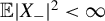 and
$\gamma <1/2$
 ,

Note that when
$(X_n, n = 1, 2, \ldots )$
 is a strictly stationary,
$\beta $
 -mixing time series and with the Hill estimator
$\overline {\gamma }=\widehat {\gamma }_{n}^{\mathrm {H}}$
 , Davison et al. (Reference Davison, Padoan and Stupfler2023) have recently proved in their Theorem 3.5 that these estimators, namely,
$\widetilde {\xi }_{\tau ^{\prime }_n}^\star (\widehat {\gamma }_{n}^{\mathrm {H}})$
 and
$\widehat {\xi }_{\tau ^{\prime }_n}^\star (\widehat {\gamma }_{n}^{\mathrm {H}})$
 , are still asymptotically Gaussian with the same rate of convergence, but at the cost of an increased asymptotic variance.
When ignoring the asymptotic bias, under the assumption
$\lambda _1=\lambda _2=0$
 , the resulting Gaussian
$100(1-\alpha )\%$
 asymptotic confidence intervals for
$\xi _{\tau ^{\prime }_n}$
 are then

with
$z_{1-\alpha /2}$
 being the quantile of level
$1-\alpha /2$
 for the standard Gaussian distribution. Bias-reduced versions of
$\widetilde {\xi }_{\tau ^{\prime }_n}^{\star }(\widehat {\gamma }_{n}^{\mathrm {H}})$
 in (A.8) and
$\widehat {\xi }_{\tau ^{\prime }_n}^{\star }(\widehat {\gamma }_{n}^{\mathrm {E}})$
 in (A.9) have been recently suggested by Girard et al. (Reference Girard, Stupfler and Usseglio-Carleve2022b) when the auxiliary function A in their SORV condition
$\mathcal {C}_2(\gamma , \rho , A)$
 takes the form
$A(t)=b\gamma t^\rho $
 for certain constants
$b\neq 0$
 and
$\rho < 0$
 . This function A can be estimated by using a consistent tail index estimator
$\overline {\gamma }$
 and the second-order parameter estimators
$ \overline {b}$
 and
$ \overline {\rho }$
 that were introduced in Gomes and Martins (Reference Gomes and Martins2002) and Fraga Alves, Gomes, and de Haan (Reference Fraga Alves, Gomes and de Haan2003). A careful consideration of the different sources of bias in the construction of
$\widetilde {\xi }_{\tau ^{\prime }_n}^{\star }$
 and
$\widehat {\xi }_{\tau ^{\prime }_n}^{\star }$
 (see Appendix B) leads to bias-reduced versions
$\widetilde {\xi }_{\tau ^{\prime }_n}^{\star ,\mathrm {BR}}(\widehat {\gamma }_{n}^{\mathrm {H},\mathrm {BR}})$
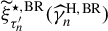 and
$\widehat {\xi }_{\tau ^{\prime }_n}^{\star ,\mathrm {BR}}(\widehat {\gamma }_{n}^{\mathrm {E},\mathrm {BR}})$
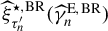 , whose full expressions are given below in (B.5) and (B.6), and with (see Caeiro, Gomes, and Pestana, Reference Caeiro, Gomes and Pestana2005)

and (see Girard et al., Reference Girard, Stupfler and Usseglio-Carleve2022a)

Gaussian
$100(1-\alpha )\%$
 asymptotic confidence intervals for
$\xi _{\tau ^{\prime }_n}$
 based on the purely asymmetric least squares estimator
$\widehat {\xi }_{\tau ^{\prime }_n}^{\star ,\mathrm {BR}}(\widehat {\gamma }_{n}^{\mathrm {E},\mathrm {BR}})$
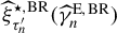 and its quantile-based competitor
$\widetilde {\xi }_{\tau ^{\prime }_n}^{\star ,\mathrm {BR}}(\widehat {\gamma }_{n}^{\mathrm {H},\mathrm {BR}})$
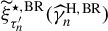 , also available as part of the R package Expectrem, are discussed in Daouia et al. (Reference Daouia, Stupfler and Usseglio-Carleve2024b), with an alternative solution put forward in Padoan and Stupfler (Reference Padoan and Stupfler2022) to correct the naive confidence intervals
$\widehat {I}_{\tau ^{\prime }_n}^{(0)}(\alpha )$
 and
$\widetilde {I}_{\tau ^{\prime }_n}^{(0)}(\alpha )$
 . We list in Appendix B the intervals constructed from Daouia et al. (Reference Daouia, Stupfler and Usseglio-Carleve2024b) as
$\widehat {I}_{\tau ^{\prime }_n}^{(1)}(\alpha )$
 ,
$\widetilde {I}_{\tau ^{\prime }_n}^{(1)}(\alpha )$
 ,
$\widehat {I}_{\tau ^{\prime }_n}^{(2)}(\alpha ),$
 and
$\widetilde {I}_{\tau ^{\prime }_n}^{(2)}(\alpha )$
 , and from Padoan and Stupfler (Reference Padoan and Stupfler2022) as
$\widehat {I}_{\tau ^{\prime }_n}^{(3)}(\alpha )$
 and
$\widetilde {I}_{\tau ^{\prime }_n}^{(3)}(\alpha )$
 . Appendix B also provides more details about these intervals and their observed finite-sample behavior.
B BIAS-REDUCED ESTIMATORS AND INFERENCE
The asymptotic distributions of
$\widetilde {\xi }_{\tau ^{\prime }_n}^{\star }(\widehat {\gamma }_{n}^{\mathrm {H}})$
 in (A.8) and
$\widehat {\xi }_{\tau ^{\prime }_n}^{\star }(\widehat {\gamma }_{n}^{\mathrm {E}})$
 in (A.9) feature bias components due to the semiparametric heavy tail framework. Bias-reduced versions of these estimators have been recently suggested by Girard et al. (Reference Girard, Stupfler and Usseglio-Carleve2022b) under the i.i.d. assumption in the particular case where the auxiliary function
$\tilde {A}$
 in their SORV condition
$\mathcal {C}_2(\gamma , \tilde {\rho }, \tilde {A})$
 takes the form
$\tilde {A}(t)=b\gamma t^{\tilde {\rho }}$
 for certain constants
$b\neq 0$
 and
$\tilde {\rho } < 0$
 . Again, in the rest of this Appendix, we set
$\rho =\tilde {\rho }$
 and
$A=\tilde {A}$
 for the sake of notational convenience.
This function A can be estimated by using a consistent tail index estimator
$\overline {\gamma }$
 and the second-order parameter estimators
$ \overline {b}$
 and
$ \overline {\rho }$
 that were introduced in Gomes and Martins (Reference Gomes and Martins2002) and Fraga Alves et al. (Reference Fraga Alves, Gomes and de Haan2003) and can directly be calculated from the R package evt0. Supplement A of Girard et al. (Reference Girard, Stupfler and Usseglio-Carleve2022b) provides a nice and comprehensive summary of how these estimators of b and
$\rho $
 are constructed. As shown by Girard et al. (Reference Girard, Stupfler and Usseglio-Carleve2022b), the direct and indirect estimators
$\widehat {\xi }_{\tau ^{\prime }_n}^\star $
 and
$\widetilde {\xi }_{\tau ^{\prime }_n}^\star $
 satisfy


To deal with the nonrandom bias term in (B.1), they have also shown that

for obvious definitions of
$B_{1,n},B_{2,n}$
 , and
$B_{3,n}$
 . As for the extrapolation bias in (B.2), they have proposed the following correction:

The terms
$B_{1,n},B_{2,n}$
 , and
$B_{3,n}$
 can be estimated by

with
$\overline {X}_n$
 being the sample mean,
$\overline {\xi }_{\tau _n}$
 either the direct intermediate estimator
$\widehat {\xi }_{\tau _n}$
 or indirect intermediate estimator
$\widetilde {\xi }_{\tau _n}$
 , and
$\overline {\xi }_{\tau ^{\prime }_n}^{\star }$
 the corresponding extrapolated version. Based on (B.1) and (B.3), the direct extrapolated estimator
$\widehat {\xi }_{\tau ^{\prime }_n}^{\star }$
 can then be corrected for its inherent bias, exclusively due to the heavy-tailed extrapolation, by the bias-reduced version,

where
$\overline {\gamma }$
 is to be itself a bias-reduced estimator of the EVI
$\gamma $
 . Similarly, from (B.2) and (B.4), a bias-corrected version of the indirect extrapolated estimator
$\widetilde {\xi }_{\tau ^{\prime }_n}^{\star }$
 is obtained as

Under
$\mathcal {C}_2(\gamma , \rho , A)$
 and additional mild regularity conditions, if
$\sqrt {n(1-\tau _{n})} (\overline {\gamma }-\gamma ) \to \Gamma $
 for a nondegenerate distribution
$\Gamma $
 , both bias-corrected estimators (B.5) and (B.6) converge in distribution to the same limit
$\Gamma $
 as
$\overline {\gamma }$
 at the slower rate
$\log ((1-\tau _n)/(1-\tau ^{\prime }_n))/\sqrt {n(1-\tau _n)}$
 , as established in Theorem 2 in Girard et al. (Reference Girard, Stupfler and Usseglio-Carleve2022b). For the choice of the bias-corrected EVI estimator
$\overline {\gamma }$
 , Girard et al. (Reference Girard, Stupfler and Usseglio-Carleve2022b) have suggested to use either the bias-reduced Hill estimator
$\widehat {\gamma }_{n}^{\mathrm {H},\mathrm {BR}}$
 in (A.10) from Caeiro et al. (Reference Caeiro, Gomes and Pestana2005), or their bias-reduced version
$\widehat {\gamma }_{n}^{\mathrm {E},\mathrm {BR}}$
 in (A.11) of
$\widehat {\gamma }_{n}^{\mathrm {E}}$
 from Girard et al. (Reference Girard, Stupfler and Usseglio-Carleve2022a). As shown in Theorem 3.1 of Caeiro et al. (Reference Caeiro, Gomes and Pestana2005), the bias-reduced Hill estimator
$\widehat {\gamma }_{n}^{\mathrm {H},\mathrm {BR}}$
 is
$\sqrt {n(1-\tau _{n})}$
 -asymptotically Gaussian with mean zero and the same variance
$\gamma ^2$
 as
$ \widehat {\gamma }_{n}^{\mathrm {H}}$
 , while
$\widehat {\gamma }_{n}^{\mathrm {E},\mathrm {BR}}$
 is
$\sqrt {n(1-\tau _{n})}$
 -asymptotically Gaussian with mean zero and variance
${\gamma ^3(1-\gamma )}\big /{(1-2\gamma )}$
 as established in Theorem 1 of Girard et al. (Reference Girard, Stupfler and Usseglio-Carleve2022b). The latter estimator is preferable variance-wise only when
$\gamma $
 is less than
$0.35$
 . The function tindexp from the R package Expectrem allows one to compute either
$\widehat {\gamma }_{n}^{E}$
 (if argument br=FALSE) or
$\widehat {\gamma }_{n}^{\mathrm {E,BR}}$
 (if br=TRUE), while the function extExpect computes the estimators
$\widehat {\xi }_{\tau ^{\prime }_n}^{\star }(\widehat {\gamma }_{n}^{E})$
 (if argument method="direct") and
$\widetilde {\xi }_{\tau ^{\prime }_n}^{\star }(\widehat {\gamma }_{n}^{H})$
 (if method="indirect") as well as their bias-reduced versions
$\widehat {\xi }_{\tau ^{\prime }_n}^{\star ,\mathrm {BR}}(\widehat {\gamma }_{n}^{\mathrm {E},\mathrm {BR}})$
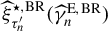 and
$\widetilde {\xi }_{\tau ^{\prime }_n}^{\star ,\mathrm {BR}}(\widehat {\gamma }_{n}^{\mathrm {H},\mathrm {BR}})$
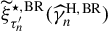 (if br=TRUE).
Gaussian
$100(1-\alpha )\%$
 asymptotic confidence intervals for
$\xi _{\tau ^{\prime }_n}$
 based on the purely asymmetric least squares estimator
$\widehat {\xi }_{\tau ^{\prime }_n}^{\star ,\mathrm {BR}}(\widehat {\gamma }_{n}^{\mathrm {E},\mathrm {BR}})$
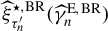 and its quantile-based competitor
$\widetilde {\xi }_{\tau ^{\prime }_n}^{\star ,\mathrm {BR}}(\widehat {\gamma }_{n}^{\mathrm {H},\mathrm {BR}})$
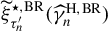 , also available as part of the R package Expectrem, are

These intervals tend, however, to have poor coverage as illustrated very recently by Daouia et al. (Reference Daouia, Stupfler and Usseglio-Carleve2024b): while the bias correction can be reasonably effective, the estimation of the variances of
$(\sqrt {n(1-\tau _n)}/\log ((1-\tau _n)/(1-\tau ^{\prime }_n))) \log (\widehat {\xi }_{\tau _n'}^{\star ,\mathrm {BR}}/\xi _{\tau _n'})$
 and
$(\sqrt {n(1-\tau _n)}/\log ((1-\tau _n)/(1-\tau ^{\prime }_n))) \log (\widetilde {\xi }_{\tau _n'}^{\star ,\mathrm {BR}}/\xi _{\tau _n'})$
 , by
$\widehat {s}_n^{2,\mathrm {BR}}$
 and
$\widetilde {\sigma }_n^{2,\mathrm {BR}}$
 , respectively, can be a long way off the truth. To improve on this, they have suggested corrected versions of
$\widehat {I}_{\tau ^{\prime }_n}^{(1)}(\alpha )$
 and
$\widetilde {I}_{\tau ^{\prime }_n}^{(1)}(\alpha )$
 defined, respectively, as

where the expressions of
$\ \widehat {s}_n^2(J)$
 and
$\widetilde {\sigma }_n^2(J)$
 , as well as the rationale behind their formulations, can be found in Daouia et al. (Reference Daouia, Stupfler and Usseglio-Carleve2024b), with
$J\ge 1$
 being a suitably chosen tuning parameter. The function CIextExpect from the R package Expectrem computes
$\widehat {I}_{\tau ^{\prime }_n}^{(2)}(\alpha )$
 with method="direct" and
$\widetilde {I}_{\tau ^{\prime }_n}^{(2)}(\alpha )$
 with method="indirect". These confidence intervals have asymptotically the desired correct coverage as established in Theorems 1 and 2 in Daouia et al. (Reference Daouia, Stupfler and Usseglio-Carleve2024b), and they serve as a benchmark for our comparison purposes in Section 3.
An alternative solution put forward earlier in Padoan and Stupfler (Reference Padoan and Stupfler2022) to correct the naive confidence intervals
$\widehat {I}_{\tau ^{\prime }_n}^{(0)}(\alpha )$
 and
$\widetilde {I}_{\tau ^{\prime }_n}^{(0)}(\alpha )$
 takes the respective forms

where
$\widehat {\xi }_{\tau ^{\prime }_n}^{\star ,\mathrm {PS}}$
 and
$\widetilde {\xi }_{\tau ^{\prime }_n}^{\star ,\mathrm {PS}}$
 (resp.,
$\overline {s}_n^{2}$
 and
$\overline {\sigma }_n^{2}$
 ) are suitably chosen bias-corrected asymmetric least squares and quantile-based estimators of the expectile
$\xi _{\tau ^{\prime }_n}$
 (resp., the asymptotic variance of
$\widehat {\xi }_{\tau ^{\prime }_n}^{\star ,\mathrm {PS}}$
 and
$\widetilde {\xi }_{\tau ^{\prime }_n}^{\star ,\mathrm {PS}}$
 ). See Padoan and Stupfler (Reference Padoan and Stupfler2022) for full details. The R function CIextExpect from the Expectrem package computes both of these confidence intervals, with method="direct_PS" for
$\widehat {I}_{\tau ^{\prime }_n}^{(3)}(\alpha )$
 and method="indirect_PS" for
$\widetilde {I}_{\tau ^{\prime }_n}^{(3)}(\alpha )$
 .
C PROOFS
We will use in the sequel the notation
$ d_n:=(1-\tau _n)/(1-\tau ^{\prime }_n) \ \text { and } \ \phi _{\gamma }(t):= \int _{1}^{t} s^{\gamma -1} \log (s) \, \mathrm {d}s. $
 We shall freely use the following fact: under condition
$\mathcal {E}_2( \gamma , \rho , a, A)$
 with
$\gamma>0$
 and
$\rho <0$
 , Theorem 3.1 in Fraga Alves et al. (Reference Fraga Alves, Gomes, de Haan and Neves2007) guarantees that there exist
$\tilde {A}$
 and
$\tilde {\rho }<0$
 such that the SORV condition
$\mathcal {C}_2(\gamma , \tilde {\rho }, \tilde A)$
 holds with
$|\tilde A|$
 being regularly varying with index
$\tilde {\rho }$
 , and
$\tilde {A}(t)\to 0$
 as
$t\to \infty $
 . Moreover, by Theorems 2.1 and 3.1 in Fraga Alves et al. (Reference Fraga Alves, Gomes, de Haan and Neves2007) in the case
$\gamma>0$
 , the auxiliary function
$\tilde {A}$
 is asymptotically proportional to
$\overline {A}(t)=a(t)/U(t)-\gamma $
 .
Proof of Theorem 1.
Write


The key argument is that the third term (C.3) converges in distribution to
$\Gamma $
 and all the other terms on the right-hand side are either
$\mathrm {o}(1)$
 or
$\mathrm {o}_{\mathbb {P}}(1)$
 , as
$n\to \infty $
 .
Indeed, since
$d_n\to \infty $
 ,
$\log (n(1-\tau ^{\prime }_n))/\sqrt {n(1-\tau _n)} \to 0$
 (as a consequence of assumptions
$n(1-\tau _n)\to \infty $
 and
$\sqrt {n(1-\tau _n)}/\log ((1-\tau _n)/(1-\tau ^{\prime }_n)) \to \infty $
 ) and
$\sqrt {n(1-\tau _n)} (\breve {\gamma }_n-\gamma )\stackrel {\mathrm {d}}{\longrightarrow } \Gamma $
 , we know by the proof of Theorem 4.3.1 on pp. 136–137 in de Haan and Ferreira (Reference de Haan and Ferreira2006) that the term (C.3) has the same limit distribution
$\Gamma $
 as
$\sqrt {n(1-\tau _n)} (\breve {\gamma }_n-\gamma )$
 (see the analysis of term II therein). In particular, since
$n(1-\tau _n)\to \infty $
 , this implies that

On the other hand, by Remark 4.3.3 on p. 135 in de Haan and Ferreira (Reference de Haan and Ferreira2006), we have

In addition, under the condition
$\mathcal {E}_2(\gamma , \rho , a, A)$
 with
$\gamma>0$
 , we have according to the proof of Theorem 1.1.6 on pp. 10–11 in de Haan and Ferreira (Reference de Haan and Ferreira2006) that
$(t-U(1/\overline {F}(t)))/a(1/\overline {F}(t))\to 0$
 as
$t\to \infty $
 . Since
$a(t)/U(t)\to \gamma $
 as
$t\to \infty $
 in view of Lemma 1.2.9 on p. 22 in de Haan and Ferreira (Reference de Haan and Ferreira2006), we conclude that
$U(1/\overline {F}(\xi _{\tau })) \sim \xi _{\tau }$
 as
$\tau \to 1$
 and then that

Thus, using (C.7), the first term (C.1) can be expressed as

Since
$\sqrt {n(1-\tau _n)}\left (\frac {\widehat {\xi }_{\tau _n}}{\xi _{\tau _n}}-1\right ) = \mathrm {O}_{\mathbb {P}}(1)$
 and
$d_n^{\gamma }\log (d_n)\to \infty $
 , the first term (C.1) is then
$\mathrm {o}_{\mathbb {P}}(1)$
 .
The second term (C.2) is handled as follows: we have by (C.6) and (C.7) that

Thus, the second term (C.2) is
$\mathrm {o}_{\mathbb {P}}(1)$
 because
$\sqrt {n(1-\tau _n)} \left ( \frac {\breve {\sigma }_n}{a(1/\overline {F}(\xi _{\tau _n}))} - 1 \right ) = \mathrm {O}_{\mathbb {P}}(1)$
 .
Let us now turn to the term (C.4) which, due to (C.7), satisfies, as
$n\to \infty $
 ,

Since condition
$\mathcal {C}_2(\gamma , \tilde {\rho }, \tilde A)$
 holds, Proposition 1 in Daouia et al. (Reference Daouia, Girard and Stupfler2018) implies that

as
$\tau \to 1$
 . It follows that
$ \frac {\overline {F}(\xi _{\tau _n})}{\overline {F}(\xi _{\tau ^{\prime }_n})}= d_n \frac {1+\varepsilon (\tau _n)}{1+\varepsilon (\tau ^{\prime }_n)} \ \text { as } n\to \infty. $
 Since
$\varepsilon (\tau )\to 0$
 as
$\tau \to 1$
 , and
$\varepsilon (\tau ^{\prime }_n)=\mathrm {O}(\varepsilon (\tau _n))$
 in view of the regular variation properties of U and of
$|\tilde {A}|$
 , a Taylor expansion yields
$ \left (\frac {\overline {F}(\xi _{\tau _n})}{d_n\overline {F}(\xi _{\tau ^{\prime }_n})}\right )^{\gamma }-1 = \mathrm {O}(\varepsilon (\tau _n)) \ \text { as } n\to \infty. $
 Thus, (C.9) becomes

It remains to show that
$\sqrt {n(1-\tau _n)} \varepsilon (\tau _n) = \mathrm {O}(1)$
 . For this, recall that
$\tilde {A}$
 is asymptotically proportional to
$t\mapsto \overline {A}(t)=a(t)/U(t)-\gamma $
 ; since
$\sqrt {n (1-\tau _n)}\, \overline {A}((1-\tau _n)^{-1})\to \mu $
 , we have
$\sqrt {n (1-\tau _n)}\, \tilde {A}((1-\tau _n)^{-1})=\mathrm {O}(1)$
 . It follows from the condition
$\sqrt {n (1-\tau _n)}/q_{\tau _n}\to \lambda _2$
 that
$\sqrt {n (1-\tau _n)}\, \varepsilon (\tau _n)=\mathrm {O}(1)$
 , and hence the term (C.4) is
$\mathrm {o}(1)$
 by (C.11).
The last term (C.5) can be rewritten as

Under
$\mathcal {E}_2(\gamma , \rho , a, A)$
 with
$\rho < 0$
 , Lemma 4.3.5 on p. 135 in de Haan and Ferreira (Reference de Haan and Ferreira2006) gives

In particular, combined with (C.8), and recalling that
$\overline {F}(\xi _{\tau _n})/\overline {F}(\xi _{\tau ^{\prime }_n}) \sim d_n\to \infty $
 , this yields

Moreover, the proof of Theorem B.3.19 on p. 401 in de Haan and Ferreira (Reference de Haan and Ferreira2006) yields
$ \lim _{t\to \infty } \frac {1}{A(1/\overline {F}(t))} \times \frac {U(1/\overline {F}(t)) - t}{a(1/\overline {F}(t))} = 0. $
 Then, on the one hand,

On the other hand, using again (C.8) together with (C.13) and the regular variation property of
$|A|$
 with index
$\rho <0$
 (see Theorem 2.3.3 on page 44 in de Haan and Ferreira, Reference de Haan and Ferreira2006), we find

As a consequence,

Then, applying again (C.7), we arrive at

Now, write
$ \sqrt {n(1-\tau _n)} A(1/\overline {F}(\xi _{\tau _n})) = \sqrt {n(1-\tau _n)} A((1-\tau _n)^{-1}) \frac {A(1/\overline {F}(\xi _{\tau _n}))}{A((1-\tau _n)^{-1})}. $
 Since
$|A|$
 is regularly varying with index
$\rho $
 and
$\overline {F}(\xi _{\tau _n})/(1-\tau _n)\to \gamma ^{-1}-1$
 , one has, by local uniformity of the regular variation property, that
$ \left | A(1/\overline {F}(\xi _{\tau _n})) \right | \sim (\gamma ^{-1}-1)^{-\rho } \left | A((1-\tau _n)^{-1}) \right | \ \text { as } n\to \infty. $
 Therefore, as
$\sqrt {n(1-\tau _n)} A((1-\tau _n)^{-1})= \mathrm {O}(1)$
 by assumption, we get

Thus, combining (C.12) and (C.14)–(C.16), we find that the last term (C.5) is indeed
$\mathrm {o}(1)$
 .
Let us now show that an equivalent statement of the convergence in Theorem 1 is

Since
$\mathcal {C}_2(\gamma , \tilde {\rho }, \tilde A)$
 holds with
$\tilde {\rho }<0$
 , we know from p. 49 in de Haan and Ferreira (Reference de Haan and Ferreira2006) that, for some constant
$\mathfrak {c}>0$
 , we have
$U(t)\sim \mathfrak {c} t^\gamma $
 as
$t \to \infty $
 . Then

Since
$\xi _{\tau }\sim (\gamma ^{-1}-1)^{-\gamma }{q_{\tau }}$
 as
$\tau \to 1$
 , we obtain the stronger version of (C.13):
$ \frac {\xi _{\tau ^{\prime }_n}}{\xi _{\tau _n}}\sim \frac {q_{\tau ^{\prime }_n}}{q_{\tau _n}}\sim d_n^{\gamma } \ \text { as } n\to \infty. $
 The desired convergence result follows by using (C.7) and (C.8).
Proof of Theorem 2.
Write

By Theorem 2.3.3 on p. 44 in de Haan and Ferreira (Reference de Haan and Ferreira2006), the function
$a(\cdot )$
 is (locally uniformly) regularly varying with index
$\gamma $
 , so that
$(1-\tau _n)/\overline {F}(\xi _{\tau _n}) = (\gamma ^{-1}-1)^{-1} + \mathrm {o}(1)$
 implies that

Hence, it suffices to show that


The first term (C.18) is
$\mathrm {O}_{\mathbb {P}}(1),$
 since
$\sqrt {n (1-\tau _n)} \left ( \frac {\widehat {a}((1-\tau _n)^{-1})}{a((1-\tau _n)^{-1})} - 1 \right ) = \mathrm {O}_{\mathbb {P}}(1),$
 and, by the consistency of
$\breve {\gamma }_n$
 as an estimator of
$\gamma \in (0,1),$
 we have
$\left (\breve {\gamma }_n^{-1}-1\right )^{-\breve {\gamma }_n} = \mathrm {O}_{\mathbb {P}}(1)$
 . Likewise, the second term (C.19) is
$\mathrm {O}_{\mathbb {P}}(1)$
 by applying the delta method in conjunction with
$\sqrt {n(1-\tau _n)} (\breve {\gamma }_n-\gamma )\stackrel {\mathrm {d}}{\longrightarrow } \Gamma $
 . As for the last term (C.20), we have again by Theorem 2.3.3 on p. 44 in de Haan and Ferreira (Reference de Haan and Ferreira2006) (and Theorem B.2.18 on page 383 in de Haan and Ferreira, Reference de Haan and Ferreira2006, which guarantees local uniformity of this SORV property) that

Moreover, from (C.10) and a Taylor expansion,

Recalling that
$\sqrt {n (1-\tau _n)} A((1-\tau _n)^{-1})=\mathrm {O}(1)$
 ,
$\sqrt {n (1-\tau _n)}/q_{\tau _n}=\mathrm {O}(1)$
 and
$\sqrt {n(1-\tau _n)} (a((1-\tau _n)^{-1})/q_{\tau _n} - \gamma ) = \mathrm {O}(1)$
 , it follows that (C.20) is
$\mathrm {O}(1)$
 as
$n\to \infty $
 , which ends the proof.
Proof of Theorem 3.
Recall from (2.9) that
$\check {\xi }_{\tau ^{\prime }_n}^{\star }=(\widehat {\gamma }_n^{-1}-1)^{-\widehat {\gamma }_n}\, \check {q}_{\tau ^{\prime }_n}^\star $
 and write


By Theorem 4.3.1 on p. 134 in de Haan and Ferreira (Reference de Haan and Ferreira2006) and the continuous mapping theorem, the first term (C.21) converges weakly to
$\Gamma /(\gamma ^{-1}-1)^{\gamma }$
 . In order to control the second term (C.22), note that since the SORV condition
$\mathcal {C}_2(\gamma , \tilde {\rho }, \tilde A)$
 holds, one has
$a(t)/U(t)\to \gamma $
 as
$t\to \infty $
 by Lemma 1.2.9 on p. 22 in de Haan and Ferreira (Reference de Haan and Ferreira2006). Using the delta method and recalling (C.7) and then (C.17), one gets

It follows that the term (C.22) is
$\mathrm {o}_{\mathbb {P}}(1)$
 . We conclude with the control of the third term: by Proposition 1 in Daouia et al. (Reference Daouia, Girard and Stupfler2020),
$ \xi _{\tau ^{\prime }_n}=(\gamma ^{-1}-1)^{-\gamma }q_{\tau ^{\prime }_n}(1+r(\tau _n')), $
 where, as
$\tau \to 1$
 ,

Recall that
$\tilde {A}$
 is asymptotically proportional to
$t\mapsto \overline {A}(t)=a(t)/U(t)-\gamma $
 ; since
$\sqrt {n (1-\tau _n)}\, \overline {A}((1-\tau _n)^{-1})\to \mu $
 by assumption, we have
$\sqrt {n (1-\tau _n)}\, \tilde {A}((1-\tau _n)^{-1})=\mathrm {O}(1)$
 , and then, from the condition
$\sqrt {n (1-\tau _n)}/q_{\tau _n}\to \lambda _2$
 and the regular variation properties of U and
$|\overline {A}|$
 , that
$\sqrt {n (1-\tau _n)}\, r(\tau _n')=\mathrm {o}(1)$
 . As a consequence,

and hence the term (C.23) is
$\mathrm {o}(1)$
 . The equivalent statement

is obtained by using once again the asymptotic proportionality relationship
$\xi _{\tau ^{\prime }_n}\sim (\gamma ^{-1}-1)^{-\gamma }q_{\tau ^{\prime }_n}$
 and arguing along the final lines of the proof of Theorem 1.
Proof of Corollary 1.
We obtain the two convergence results by applying Theorem 1. To do so, we first need to show that the last condition of this theorem is satisfied. Recall that under assumption
$\mathcal {E}_2$
 and the tail-heaviness condition (2.2) with
$0<\gamma <1/2$
 , condition
$\mathcal {C}_2$
 is satisfied. Then, under the assumptions that
$\mathbb {E}|X_{-}|^2<\infty $
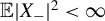 ,
$\tau _n=1-k_n/n\to 1$
 with
$n(1-\tau _n)=k_n\to \infty $
 and
$\sqrt {n(1-\tau _n)}\tilde {A}((1-\tau _n)^{-1}) = \mathrm {O}(1)$
 , one has, by Theorem 1 in Daouia et al. (Reference Daouia, Girard and Stupfler2020), that

Note that
$\sqrt {n(1-\tau _n)}\tilde {A}((1-\tau _n)^{-1}) = \mathrm {O}(1)$
 is guaranteed by the condition
$\sqrt {n(1-\tau _n)} (a ((1-\tau _n)^{-1})/q_{\tau _n} - \gamma ) \to \mu \in \mathbb {R}$
 , see the proof of Theorem 1. Then, according to Theorem 2, it suffices to show that the two conditions of this theorem hold for both the GPML and Moment estimators of
$a(n/k_n)$
 and
$\gamma $
 . Following Theorem 3.4.2 on p. 92 in de Haan and Ferreira (Reference de Haan and Ferreira2006), the GPML estimators satisfy the joint convergence (2.12) and hence we obtain

where
$\Gamma ^{\mathrm {ML}}$
 is the normal distribution
$\mathcal {N}\left ( \frac {\lambda _1(1+\gamma )}{(1-\rho )(1+\gamma -\rho )}, (1+\gamma )^2\right )$
 . On the other hand, under the first condition of Theorem 1, we know from Lemma B.3.16 on p. 397 in de Haan and Ferreira (Reference de Haan and Ferreira2006) that a second-order condition
$\mathcal {E}_2(\gamma _{-}=0, \rho , a/U, Q)$
 holds for
$\log U(t)$
 with an auxiliary function Q defined by

where the quantity l is defined as
$l=\lim _{t\to \infty } U(t)-a(t)/\gamma $
 , see Theorem 2.1 in Fraga Alves et al. (Reference Fraga Alves, Gomes, de Haan and Neves2007) for the existence of this limit. Then, as
$n\to \infty $
 ,

Therefore, all conditions of Corollary 4.2.2 on p. 133 in de Haan and Ferreira (Reference de Haan and Ferreira2006) are satisfied, which yields the joint convergence (2.13), and so we obtain

where, by Theorem 3.5.4 on p. 104 in de Haan and Ferreira (Reference de Haan and Ferreira2006),
$\Gamma ^{\mathrm {Mom}}$
 stands for the normal distribution
$\mathcal {N}\left ( \lambda ^{\mathrm {Mom}} b_{\gamma ,\rho }, \gamma ^2+1\right )$
 , with

Thus, by applying Theorem 2 in conjunction with (C.25) and (C.26), and then Theorem 1 in conjunction with (C.24), we get

Since
$\breve {\sigma }_n^{\mathrm {ML}}/a(1/\overline {F}(\xi _{\tau _n}))\stackrel {\mathbb {P}}{\longrightarrow } 1$
 and
$\breve {\sigma }_n^{\mathrm {Mom}}/a(1/\overline {F}(\xi _{\tau _n}))\stackrel {\mathbb {P}}{\longrightarrow } 1$
 , and since
$\phi _{\widehat {\gamma }_n^{\mathrm {ML}}}(d_n)/ \phi _{\gamma }(d_n)\stackrel {\mathbb {P}}{\longrightarrow } 1$
 and
$\phi _{\widehat {\gamma }_n^{\mathrm {Mom}}}(d_n)/ \phi _{\gamma }(d_n)\stackrel {\mathbb {P}}{\longrightarrow } 1$
 in view of Corollary 4.3.2 on p. 135 in de Haan and Ferreira (Reference de Haan and Ferreira2006), the conclusion follows by using Slutsky’s lemma.
Proof of Corollary 2.
According to Section 4.3.1 in de Haan and Ferreira (Reference de Haan and Ferreira2006), see pp. 139–140, we have, under the first three conditions of Theorem 3, when the scale and shape GPML estimators are used, that
$ \frac {\sqrt {k_n}}{a(n/k_n)\phi _{\gamma }(d_n)} ({\check {q}_{\tau ^{\prime }_n}^\star }-q_{\tau ^{\prime }_n})\stackrel {\mathrm {d}}{\longrightarrow } \Gamma ^{\mathrm {ML}}. $
 Then, following the proof of Theorem 3, we obtain
$ \sqrt {k_n} \frac {\check {\xi }_{\tau ^{\prime }_n}^{\star }(\widehat {\gamma }_n^{\mathrm {ML}},\widehat {\sigma }_n^{\mathrm {ML}}) - \xi _{\tau ^{\prime }_n}}{a(n/k_n) \phi _{\gamma }(d_n)} \stackrel {\mathrm {d}}{\longrightarrow } \frac {\Gamma ^{\mathrm {ML}}}{(\gamma ^{-1}-1)^{\gamma }}. $
 Besides, as seen in the proof of Corollary 1, under the first and second conditions of Theorem 3, the Moment estimators satisfy the joint convergence (2.13) that corresponds to our last required condition of Theorem 3. Therefore,

Since
$\widehat {\sigma }_n^{\mathrm {ML}}/a(n/k_n)\stackrel {\mathbb {P}}{\longrightarrow } 1$
 ,
$\phi _{\widehat {\gamma }_n^{\mathrm {ML}}}(d_n)/ \phi _{\gamma }(d_n)\stackrel {\mathbb {P}}{\longrightarrow } 1$
 ,
$\widehat {\sigma }_n^{\mathrm {Mom}}/a(n/k_n)\stackrel {\mathbb {P}}{\longrightarrow } 1$
 , and
$\phi _{\widehat {\gamma }_n^{\mathrm {Mom}}}(d_n)/ \phi _{\gamma }(d_n)\stackrel {\mathbb {P}}{\longrightarrow } 1$
 , the proof is complete following a use of Slutsky’s lemma.
FUNDING STATEMENT
This research was supported by the French National Research Agency under the grants ANR-18-EURE-0023 (EUR MINT), ANR-17-EURE-0010 (EUR CHESS, Investissements d’Avenir Program), ANR-23-CE40-0009 (EXSTA Project), and ANR-11-LABX-0020-01 (Centre Henri Lebesgue). G.S. acknowledges further support from the Chair Stress Test, RISK Management and Financial Steering of the Foundation Ecole Polytechnique .
COMPETING INTERESTS
The authors declare that no competing interests exist.