1 Introduction
Liquid jets spiralling out under the action of centrifugal forces are elements of many applications, including spinning disc atomization (Senuma et al. Reference Senuma, Lowe, Zweifel, Hilborn and Marison2000), drawing and spinning of polymers and glass (Pearson Reference Pearson1985), nanofibre formation (Mellado, McIlwee & Badrossamay Reference Mellado, McIlwee and Badrossamay2011), prilling (Saleh et al. Reference Saleh, Ahmed, Al-Mosuli and Barghi2015) among others. Theoretical research into the dynamics of curved and later spiralling liquid jets began with integral approaches (Entov & Yarin Reference Entov and Yarin1984; Tchavdarov, Yarin & Radev Reference Tchavdarov, Yarin and Radev1993) and then moved on to a more detailed description, first, of nearly straight jets (Dewynne, Ockendon & Wilmott Reference Dewynne, Ockendon and Wilmott1992; Cummings & Howell Reference Cummings and Howell1999) and then arbitrarily curved ones, including the effects of inertia and surface tension (Wallwork et al. Reference Wallwork, Decent, King and Schulkes2002), gravity (Decent, King & Wallwork Reference Decent, King and Wallwork2002), viscosity with no gravity (Decent et al. Reference Decent, King, Simmons, Părău, Wallwork, Gurney and Uddin2009), unsteadiness and arbitrary shape of the jet’s trajectory, first, without surface tension (Panda, Marheineke & Wegener Reference Panda, Marheineke and Wegener2008) and then with surface tension (Marheineke & Wegener Reference Marheineke and Wegener2009), propagation of waves (Părău et al. Reference Părău, Decent, King, Simmons and Wong2006), viscoelasticity (Alsharif, Uddin & Afzaal Reference Alsharif, Uddin and Afzaal2015; Marheineke et al. Reference Marheineke, Liljegren-Sailer, Lorenz and Wegener2016), surfactants for Newtonian (Uddin, Decent & Simmons Reference Uddin, Decent and Simmons2008) and non-Newtonian fluids (Uddin & Decent Reference Uddin and Decent2009) to mention only the main developments. All this research activity gives an impression of a well-researched topic with plenty of results ripe for application to problems where the spiralling jet is but one element of the flow and ready-to-use simplified equations and/or solutions are required.
However, there is one serious issue. To be confident in the results one finds in the literature with regard to their potential application, one should be able to verify at least some key elements in their derivation. The problem in question is mathematically rather intricate, by necessity it requires the use of a local curvilinear non-orthogonal coordinate system, and one should be able to check, for example, how the authors of published work handled the derivatives of the non-orthogonal basis vectors of this system with respect to these curvilinear non-orthogonal coordinates, which is needed to do covariant differentiation in the derivation of the governing equations of fluid mechanics. However, it is these details that are invariably missing in the exposition of published studies. Furthermore, and rather alarmingly, the demonstrably non-orthogonal coordinate system, which has been known as such for quite a while (Entov & Yarin Reference Entov and Yarin1984), is routinely referred to and dealt with as orthogonal (Decent et al. Reference Decent, King and Wallwork2002; Panda et al. Reference Panda, Marheineke and Wegener2008; Marheineke & Wegener Reference Marheineke and Wegener2009; Marheineke et al. Reference Marheineke, Liljegren-Sailer, Lorenz and Wegener2016). Such details as, for example, differentiation of one independent variable with respect to another, as in (20) of Decent et al. (Reference Decent, King and Wallwork2002), or a kinematic boundary condition on the free surface somehow including a component of the binormal to the trajectory, as (2.7) in Wallwork et al. (Reference Wallwork, Decent, King and Schulkes2002), do little to reassure the reader.
Thus, a ‘practitioner’ looking for results to apply faces a dilemma: either to suppress unease and take what has been published on trust or to spend the same amount of time and effort as the authors did rederiving them to make sure they are correct. Neither of these options looks particularly appealing. The first one essentially means leaving science, as then there would be only faith to rely upon, whilst the second largely defeats the whole point of mathematical research where verification and replication of obtained results is supposed to be much easier, and by far less time consuming, than their original derivation.
If one sets aside these reservations and embarks on a laborious journey of deriving the mathematical framework needed to handle the spiralling jet problem and then goes through the reported derivations and solutions, it becomes clear very soon that taking the published results on trust would have been, at best, unwise. For example, the entire research output of Decent and co-workers in this area (Decent et al. Reference Decent, King and Wallwork2002; Wallwork et al. Reference Wallwork, Decent, King and Schulkes2002; Partridge et al. Reference Partridge, Wong, Simmons, Părău and Decent2005; Părău et al. Reference Părău, Decent, King, Simmons and Wong2006, Reference Părău, Decent, Simmons, Wong and King2007; Uddin, Decent & Simmons Reference Uddin, Decent and Simmons2006; Uddin et al. Reference Uddin, Decent and Simmons2008; Decent et al. Reference Decent, King, Simmons, Părău, Wallwork, Gurney and Uddin2009; Uddin & Decent Reference Uddin and Decent2009; Hawkins et al. Reference Hawkins, Gurney, Decent, Simmons and Uddin2010; Uddin & Decent Reference Uddin and Decent2012) appears to be riddled with mistakes, which begin with the handling of some basic elements of differential geometry required in this problem (see below for details). Furthermore, the mistakes tend to propagate in all directions as later papers rely on those published earlier, with cross-referencing between different research groups, so that these, purely mathematical, errors ‘snowball’ and make distilling the results potentially unaffected by them a practically impossible task, especially given an abbreviated format of the exposition of mathematics. The bottom line to our trawling of the work published on the dynamics of spiralling jets is that we were unable to find a single paper with correct mathematics, not to mention a verifiable exposition. The ‘bifurcation point’ after which valid early work on buckling (Entov & Yarin Reference Entov and Yarin1984; Tchavdarov et al. Reference Tchavdarov, Yarin and Radev1993) and nearly straight jets (Dewynne et al. Reference Dewynne, Ockendon and Wilmott1992; Cummings & Howell Reference Cummings and Howell1999) turned into a stream of erroneous publications on spiralling and highly curved jets appears to be Wallwork et al. (Reference Wallwork, Decent, King and Schulkes2002) so that now, after fifteen years of erroneous mathematical exercises, the field is in need of a thorough clean up.
The purpose of the present work is twofold. Firstly, it is to create a verifiable mathematical framework for the spiralling jet problem, a framework that does not use any simplifying assumptions with the exposition allowing one to check its every element without even reaching for pen and paper. Transparency of the exposition here is the key given that, as we show, too many mistakes in the published work are hidden behind reassuring phrases such as ‘using standard methods, we obtain
 $\ldots$
’. Our intention is (i) to give researchers and ‘practitioners’ in this field the necessary mathematical toolkit to deal with different aspects of the curved jet problem and (ii) to set the standard of clarity of exposition required in this field for it to develop. The transparent mathematical framework we present also makes it possible to analyse the key elements where mistakes are typically made. In order for this analysis not to interfere with our exposition of the results, we place it in separate subsections at the end of the key steps in the derivation.
The second aim of the present work is to examine the case most important from a practical viewpoint, namely that of a slender jet, where we asymptotically derive some equations needed for practical applications. These include, first, equations for the jet’s trajectory, which come from solving the governing equations for a steady flow. Secondly, we derive the simple one-dimensional model describing the propagation of peristaltic disturbances, which allows one to consider evolution of the flow leading to the formation of drops. Both types of equations are derived for different relations between the slenderness parameter and the Weber number, with assumptions highlighted throughout the derivation.
Ultimately, our goal is to show that spiralling jets, or indeed jets of arbitrary shape, are very easy to handle. Once the Frenet basis is used alongside the, generally non-orthogonal, jet-specific coordinate system with respect to which the flow velocity is considered, the mathematics required is no more difficult than that involved in the description of the motion of a material point in the Frenet basis. This analogy is pointed out in the places where the key equations are introduced. As for the disturbances that propagate along the jet, it is shown that their wavelengths are asymptotically short compared with the radius of curvature of the jet’s trajectory, so that for them, to leading order in the slenderness parameter, the jet is straight. The general formulation makes it possible to consider higher-order approximations in the slenderness parameter, where the curvature of the jet’s trajectory comes into play, or to abandon the slender-jet approximation altogether.
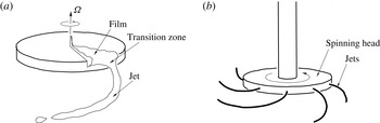
Sketches of applications involving spiralling liquid jets: (a) a representative sector in the ligament regime of the spinning disc atomization process (Frost Reference Frost1981), (b) the generation of nanofibres from a spinning head (Zhang & Lu Reference Zhang and Lu2014).

The structure of the present work is as follows. In § 2, we state what problem is to be considered and in § 3 lay out the necessary geometric framework, from the introduction of the local jet-specific coordinate system, the basis vectors and components of the metric tensor to the calculation of the Christoffel symbols and the free-surface curvature in a general case, i.e. without assuming that the jet is slender. For the ease of reading, we place some technical details of the calculations into appendices, which form an integral part of this paper. In § 4, the governing equations and boundary conditions of § 2 are derived for the local jet-specific curvilinear coordinate system in a general case, and § 5 deals with these equations in the slender-jet approximation, where we derive ordinary differential equations for the jet’s trajectory in different cases and one-dimensional equations describing peristaltic disturbances. In § 6, we summarize the work, point out some directions of research that it makes possible and highlight the necessity of developing a purpose-designed symbolic software capable of converting the invariant vector/tensor form of fluid mechanics equations into their scalar form corresponding to a prescribed curvilinear coordinate system.
2 Problem
We consider a free liquid jet produced by some kind of spinning device. It could be, for example, a spinning disc atomizer, where, in the so-called ‘full ligament mode’, the film flowing over a rotating disc comes out of its rim in the form of separate jets (figure 1
a), or the nanofibre generator, where the jets come from the orifices in the side wall of a rapidly spinning head (figure 1
b). The gas surrounding the jet is assumed to be inviscid and dynamically passive. In the simplest case of a device spinning with a constant angular velocity about a vertical axis directed against gravity
 $\boldsymbol{g}$
and the fluid modelled as inviscid and incompressible with a constant density
 $\unicode[STIX]{x1D70C}$
, the fluid’s velocity
 $\boldsymbol{v}$
and pressure
 $p$
(measured with respect to a constant pressure in the ambient gas) are described by the Euler equations which, in the observer’s reference frame rotating with angular velocity
 $\unicode[STIX]{x1D734}$
and with the origin at the axis of rotation, take the form:
 $$\begin{eqnarray}\unicode[STIX]{x1D735}\boldsymbol{\cdot }\boldsymbol{v}=0,\quad \frac{\text{d}\boldsymbol{v}}{\text{d}t}=-\frac{1}{\unicode[STIX]{x1D70C}}\unicode[STIX]{x1D735}p+\boldsymbol{g}-2\unicode[STIX]{x1D734}\times \boldsymbol{v}-\unicode[STIX]{x1D734}\times (\unicode[STIX]{x1D734}\times \boldsymbol{r}),\end{eqnarray}$$
where
 $\boldsymbol{r}$
is the radius vector, the last term on the right-hand side is the centrifugal force and the preceding term is the Coriolis force. Note that, to consider the jet as a whole as steady, in (2.1)
 $\unicode[STIX]{x1D734}$
must be the angular velocity of the frame rotating with the jet, which is usually, as in the situation shown in figure 1(b), equal to the angular velocity of the device, but in some cases, notably in the spinning disc atomization process (figure 1
a), can be different, albeit not by much.
On the free surface of the jet implicitly given as
 $f(\boldsymbol{r},t)=0$
, where the function
 $f$
is to be found, one has the usual kinematic and dynamic boundary conditions:
 $$\begin{eqnarray}\displaystyle & \displaystyle \frac{\unicode[STIX]{x2202}f}{\unicode[STIX]{x2202}t}+\boldsymbol{v}\boldsymbol{\cdot }\unicode[STIX]{x1D735}f=0, & \displaystyle\end{eqnarray}$$
 $$\begin{eqnarray}\displaystyle & \displaystyle p=\unicode[STIX]{x1D70E}\unicode[STIX]{x1D705}_{s}, & \displaystyle\end{eqnarray}$$
where
 $\unicode[STIX]{x1D70E}$
is the surface tension and
 $\unicode[STIX]{x1D705}_{s}$
is the mean curvature of the jet’s free surface.
To specify a particular flow, one has to add to the system (2.1)–(2.3) also the boundary conditions specifying how the jet is produced, e.g. at the orifice of the spinning container, and initial conditions specifying the initial shape of the jet’s free surface and the initial distribution of velocity. Here, we will be interested in (2.1)–(2.3) and the equations one can derive for the jet’s trajectory and the nonlinear disturbances propagating along the jet.
3 Geometric framework
To describe the flow in the jet, it is convenient to consider equations (2.1) and boundary conditions (2.2), (2.3) in a local curvilinear coordinate system based on some line that goes along the jet and whose form is to be determined. Such a ‘jet-specific’ coordinate system would allow one to introduce meaningful scales along and across the jet and, using their disparity in the slender-jet case, simplify the problem via an appropriate asymptotic method. The price to pay for this simplification is that one has to handle a rather cumbersome geometric side of the problem in a systematic way.
3.1 Baseline and Frenet’s basis
Let us introduce the jet’s ‘baseline’, i.e. a geometric line going along the jet and, for the class of motions to be considered, staying inside it at all times, as
 $$\begin{eqnarray}\boldsymbol{R}(\unicode[STIX]{x1D709})=X(\unicode[STIX]{x1D709})\,\hat{\boldsymbol{x}}+Y(\unicode[STIX]{x1D709})\,\hat{\boldsymbol{y}}+Z(\unicode[STIX]{x1D709})\,\hat{\boldsymbol{z}},\end{eqnarray}$$
where
 $\unicode[STIX]{x1D709}$
is the arclength along it and
 $\hat{\boldsymbol{x}}$
,
 $\hat{\boldsymbol{y}}$
and
 $\hat{\boldsymbol{z}}$
are the basis vectors of the Cartesian coordinate frame rotating with the angular velocity
 $\unicode[STIX]{x1D734}$
, i.e. the frame in which we have equations (2.1). We introduce the term ‘baseline’ as opposed to ‘centreline’ used for (3.1) in the literature to emphasize that the ‘baseline’ is a geometric construction needed to set-up a local coordinate system whilst the location of the jet’s ‘centreline’, if the ‘centre’ of an arbitrarily shaped cross-section of the jet can be meaningfully defined, is determined by the jet’s dynamics so that, in particular, one can have a situation where the ‘centreline’ wobbles about the defined-as-steady ‘baseline’. In what follows, we will assume that the functions
 $X(\unicode[STIX]{x1D709})$
,
 $Y(\unicode[STIX]{x1D709})$
,
 $Z(\unicode[STIX]{x1D709})$
are sufficiently smooth with all derivatives required of them continuous.
The Frenet (or ‘natural’) local orthonormal basis at every point of the baseline is formed by the unit tangential vector
 $\unicode[STIX]{x1D749}(\unicode[STIX]{x1D709})$
, the unit normal vector
 $\boldsymbol{n}(\unicode[STIX]{x1D709})$
and the unit binormal vector
 $\boldsymbol{b}(\unicode[STIX]{x1D709})$
defined in terms of
 $\boldsymbol{R}(\unicode[STIX]{x1D709})$
and its components as follows:
 $$\begin{eqnarray}\displaystyle \unicode[STIX]{x1D749}=\frac{\text{d}\boldsymbol{R}}{\text{d}\unicode[STIX]{x1D709}}=X^{\prime }(\unicode[STIX]{x1D709})\hat{\boldsymbol{x}}+Y^{\prime }(\unicode[STIX]{x1D709})\hat{\boldsymbol{y}}+Z^{\prime }(\unicode[STIX]{x1D709})\hat{\boldsymbol{z}},\quad X^{\prime 2}+Y^{\prime 2}+Z^{\prime 2}=1, & & \displaystyle\end{eqnarray}$$
 $$\begin{eqnarray}\displaystyle & \displaystyle \boldsymbol{n}=\frac{\text{d}\unicode[STIX]{x1D749}}{\text{d}\unicode[STIX]{x1D709}}\left|\frac{\text{d}\unicode[STIX]{x1D749}}{\text{d}\unicode[STIX]{x1D709}}\right|^{-1}=\frac{\text{d}^{2}\boldsymbol{R}}{\text{d}\unicode[STIX]{x1D709}^{2}}\left|\frac{\text{d}^{2}\boldsymbol{R}}{\text{d}\unicode[STIX]{x1D709}^{2}}\right|^{-1}=\frac{X^{\prime \prime }\hat{\boldsymbol{x}}+Y^{\prime \prime }\hat{\boldsymbol{y}}+Z^{\prime \prime }\hat{\boldsymbol{z}}}{\sqrt{X^{\prime \prime 2}+Y^{\prime \prime 2}+Z^{\prime \prime 2}}} & \displaystyle\end{eqnarray}$$
 $$\begin{eqnarray}\displaystyle & \displaystyle \boldsymbol{b}=\unicode[STIX]{x1D749}\times \boldsymbol{n}=\frac{(Y^{\prime }Z^{\prime \prime }-Z^{\prime }Y^{\prime \prime })\,\hat{\boldsymbol{x}}+(Z^{\prime }X^{\prime \prime }-X^{\prime }Z^{\prime \prime })\,\hat{\boldsymbol{y}}+(X^{\prime }Y^{\prime \prime }-Y^{\prime }X^{\prime \prime })\,\hat{\boldsymbol{z}}}{\sqrt{X^{\prime \prime 2}+Y^{\prime \prime 2}+Z^{\prime \prime 2}}}, & \displaystyle\end{eqnarray}$$
where primes denote differentiation with respect to
 $\unicode[STIX]{x1D709}$
. The second equation in (3.2) specifies that
 $\unicode[STIX]{x1D709}$
is the arclength. The Frenet basis is often used in the mechanics of a material point in situations where the point’s trajectory is known (e.g. in designing a roller-coaster track) as it allows one to reduce the problem of determining three unknown components of velocity to a one-dimensional problem along the trajectory with the normal and binormal projections of the equations of motion used a posteriori to find the reaction forces (Butenin, Lunz & Merkin Reference Butenin, Lunz and Merkin1979).
The derivatives of the tangent, normal and binormal with respect to
 $\unicode[STIX]{x1D709}$
are related with
 $\unicode[STIX]{x1D749}$
,
 $\boldsymbol{n}$
and
 $\boldsymbol{b}$
via the Frenet formulae:
 $$\begin{eqnarray}\frac{\text{d}\unicode[STIX]{x1D749}}{\text{d}\unicode[STIX]{x1D709}}=\unicode[STIX]{x1D705}_{1}\boldsymbol{n},\quad \frac{\text{d}\boldsymbol{n}}{\text{d}\unicode[STIX]{x1D709}}=-\unicode[STIX]{x1D705}_{1}\unicode[STIX]{x1D749}+\unicode[STIX]{x1D705}_{2}\boldsymbol{b},\quad \frac{\text{d}\boldsymbol{b}}{\text{d}\unicode[STIX]{x1D709}}=-\unicode[STIX]{x1D705}_{2}\boldsymbol{n},\end{eqnarray}$$
where
 $$\begin{eqnarray}\unicode[STIX]{x1D705}_{1}(\unicode[STIX]{x1D709})=\left|\frac{\text{d}^{2}\boldsymbol{R}}{\text{d}\unicode[STIX]{x1D709}^{2}}\right|=\sqrt{X^{\prime \prime 2}+Y^{\prime \prime 2}+Z^{\prime \prime 2}},\end{eqnarray}$$
 $$\begin{eqnarray}\displaystyle \unicode[STIX]{x1D705}_{2} & = & \displaystyle \left\langle \frac{\text{d}\boldsymbol{R}}{\text{d}\unicode[STIX]{x1D709}},\frac{\text{d}^{2}\boldsymbol{R}}{\text{d}\unicode[STIX]{x1D709}^{2}},\frac{\text{d}^{3}\boldsymbol{R}}{\text{d}\unicode[STIX]{x1D709}^{3}}\right\rangle \left|\frac{\text{d}\boldsymbol{R}}{\text{d}\unicode[STIX]{x1D709}}\times \frac{\text{d}^{2}\boldsymbol{R}}{\text{d}\unicode[STIX]{x1D709}^{2}}\right|^{-2}\nonumber\\ \displaystyle & = & \displaystyle \frac{X^{\prime }(Y^{\prime \prime }Z^{\prime \prime \prime }-Z^{\prime \prime }Y^{\prime \prime \prime })+Y^{\prime }(Z^{\prime \prime }X^{\prime \prime \prime }-X^{\prime \prime }Z^{\prime \prime \prime })+Z^{\prime }(X^{\prime \prime }Y^{\prime \prime \prime }-Y^{\prime \prime }X^{\prime \prime \prime })}{(Y^{\prime }Z^{\prime \prime }-Z^{\prime }Y^{\prime \prime })^{2}+(Z^{\prime }X^{\prime \prime }-X^{\prime }Z^{\prime \prime })^{2}+(X^{\prime }Y^{\prime \prime }-Y^{\prime }X^{\prime \prime })^{2}}\end{eqnarray}$$
are the curvature and the torsion of the baseline, respectively. In the last equation, the angular brackets denote the so-called parallelepipedal product, i.e. the determinant where the components of the three vectors inside the brackets form the rows.
3.2 Local curvilinear coordinates and the corresponding basis
To be able to describe the flow, we introduce a local curvilinear coordinate system
 $(\unicode[STIX]{x1D709},\unicode[STIX]{x1D702},\unicode[STIX]{x1D703})$
where
 $\unicode[STIX]{x1D709}$
is the arclength along the baseline introduced earlier and
 $\unicode[STIX]{x1D702}$
and
 $\unicode[STIX]{x1D703}$
are the polar radius and angle in the plane normal to the baseline at point
 $\boldsymbol{R}(\unicode[STIX]{x1D709})$
, i.e. the plane where
 $\boldsymbol{n}(\unicode[STIX]{x1D709})$
and
 $\boldsymbol{b}(\unicode[STIX]{x1D709})$
lie, with the angle
 $\unicode[STIX]{x1D703}$
measured from
 $\boldsymbol{n}$
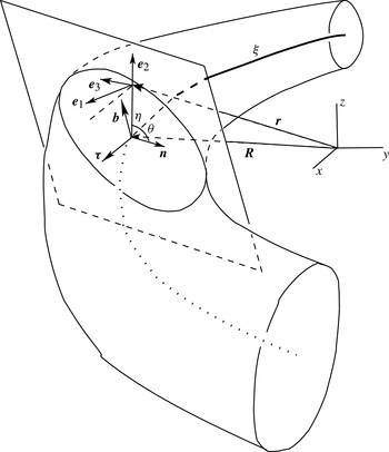
(figure 2). Where convenient, we will also use the notation
 $\unicode[STIX]{x1D709}^{1}=\unicode[STIX]{x1D709}$
,
 $\unicode[STIX]{x1D709}^{2}=\unicode[STIX]{x1D702}$
,
 $\unicode[STIX]{x1D709}^{3}=\unicode[STIX]{x1D703}$
and the summation convention with respect to repeated lower and upper indices.
In the reference frame rotating with the angular velocity
 $\unicode[STIX]{x1D734}$
, the radius vector of an arbitrary point in the jet in Cartesian coordinates
 $(x,y,z)$
is given by
 $$\begin{eqnarray}\boldsymbol{r}(x,y,z)=x\,\hat{\boldsymbol{x}}+y\,\hat{\boldsymbol{y}}+z\,\hat{\boldsymbol{z}},\end{eqnarray}$$
and the same radius-vector is expressed in the local coordinates
 $(\unicode[STIX]{x1D709},\unicode[STIX]{x1D702},\unicode[STIX]{x1D703})$
as
 $$\begin{eqnarray}\boldsymbol{r}(\unicode[STIX]{x1D709},\unicode[STIX]{x1D702},\unicode[STIX]{x1D703})=\boldsymbol{R}(\unicode[STIX]{x1D709})+\unicode[STIX]{x1D702}\cos \unicode[STIX]{x1D703}\,\boldsymbol{n}(\unicode[STIX]{x1D709})+\unicode[STIX]{x1D702}\sin \unicode[STIX]{x1D703}\,\boldsymbol{b}(\unicode[STIX]{x1D709}).\end{eqnarray}$$
Expressions (3.8) and (3.9) allow one to recalculate one set of coordinates into the other. The local coordinate system, which we have introduced via (3.9), can be used for the jets in situations where the normal planes to the baseline do not intersect inside the jet and hence the local coordinates of all points inside the jet and on its surface are specified uniquely. In other words, the radius of curvature of the baseline must be greater than the distance from it to the concave side of the jet’s free surface, which can be achieved by the appropriate choice of the baseline.
A sketch illustrating coordinate systems involved in the description of curved jets. The arclength
 $\unicode[STIX]{x1D709}~(=\unicode[STIX]{x1D709}^{1})$
along the jet’s ‘baseline’ together with two orthogonal (e.g. plane polar) coordinates
 $\unicode[STIX]{x1D702}~(=\unicode[STIX]{x1D709}^{2})$
,
 $\unicode[STIX]{x1D703}~(=\unicode[STIX]{x1D709}^{3})$
in the plane normal to the baseline give a visual impression of an always-orthogonal coordinate system, often declared as such ‘by definition’ (Decent et al.
Reference Decent, King and Wallwork2002) with the tangent to the baseline
 $\unicode[STIX]{x1D749}=\text{d}\boldsymbol{R}/\text{d}\unicode[STIX]{x1D709}$
‘defined’ as the basis vector corresponding to the
 $\unicode[STIX]{x1D709}$
-coordinate. However, once defined analytically in the correct way as the derivative of the radius vector
 $\boldsymbol{r}$
with respect to
 $\unicode[STIX]{x1D709}$
(3.10), the basis vector
 $\boldsymbol{e}_{1}$
corresponding to the
 $\unicode[STIX]{x1D709}$
-coordinate turns out to coincide with
 $\unicode[STIX]{x1D749}$
only on the baseline whilst away from it
 $\boldsymbol{e}_{1}$
appears to be different in magnitude and can even have a non-zero projection on the azimuthal direction
 $(\boldsymbol{e}_{1}\boldsymbol{\cdot }\boldsymbol{e}_{3}=\unicode[STIX]{x1D702}^{2}\unicode[STIX]{x1D705}_{2}\neq 0)$
if the baseline’s torsion
 $\unicode[STIX]{x1D705}_{2}$
is non-zero. Thus, unlike the orthonormal Frenet basis
 $\unicode[STIX]{x1D749}$
,
 $\boldsymbol{n}$
,
 $\boldsymbol{b}$
, in general, i.e. for a non-zero torsion of the baseline
 $(\unicode[STIX]{x1D705}_{2}\neq 0)$
, the coordinate system
 $(\unicode[STIX]{x1D709},\unicode[STIX]{x1D702},\unicode[STIX]{x1D703})$
, whose basis is shown as
 $\boldsymbol{e}_{1}$
,
 $\boldsymbol{e}_{2}$
,
 $\boldsymbol{e}_{3}$
, is non-orthogonal and hence cannot be handled in terms of ‘scaling factors’ (i.e. Lamé coefficients) nor via transformations based on its presumed orthogonality.

Essentially from this point onwards, i.e. after we have introduced the local coordinate system by (3.9), the construction of the mathematical framework for our problem is ‘automatic’ in the sense that one just has to follow the rules of differential geometry.
The basis vectors of our curvilinear coordinate system are defined by
 $$\begin{eqnarray}\boldsymbol{e}_{i}=\frac{\unicode[STIX]{x2202}\boldsymbol{r}}{\unicode[STIX]{x2202}\unicode[STIX]{x1D709}^{i}}\quad (i=1,2,3),\end{eqnarray}$$
i.e. as tangent (and not necessarily unit) vectors to the corresponding coordinate lines. Using (3.9) and Frenet’s formulae (3.5), we have
 $$\begin{eqnarray}\displaystyle \boldsymbol{e}_{1} & = & \displaystyle \frac{\unicode[STIX]{x2202}\boldsymbol{r}}{\unicode[STIX]{x2202}\unicode[STIX]{x1D709}}=\frac{\text{d}\boldsymbol{R}}{\text{d}\unicode[STIX]{x1D709}}+\unicode[STIX]{x1D702}\cos \unicode[STIX]{x1D703}\frac{\text{d}\boldsymbol{n}}{\text{d}\unicode[STIX]{x1D709}}+\unicode[STIX]{x1D702}\sin \unicode[STIX]{x1D703}\frac{\text{d}\boldsymbol{b}}{\text{d}\unicode[STIX]{x1D709}}=\unicode[STIX]{x1D749}+\unicode[STIX]{x1D702}\cos \unicode[STIX]{x1D703}(-\unicode[STIX]{x1D705}_{1}\unicode[STIX]{x1D749}+\unicode[STIX]{x1D705}_{2}\boldsymbol{b})+\unicode[STIX]{x1D702}\sin \unicode[STIX]{x1D703}(-\unicode[STIX]{x1D705}_{2}\boldsymbol{n})\nonumber\\ \displaystyle & = & \displaystyle (1-\unicode[STIX]{x1D702}\unicode[STIX]{x1D705}_{1}\cos \unicode[STIX]{x1D703})\unicode[STIX]{x1D749}-\unicode[STIX]{x1D702}\unicode[STIX]{x1D705}_{2}\sin \unicode[STIX]{x1D703}\,\boldsymbol{n}+\unicode[STIX]{x1D702}\unicode[STIX]{x1D705}_{2}\cos \unicode[STIX]{x1D703}\,\boldsymbol{b},\end{eqnarray}$$
 $$\begin{eqnarray}\displaystyle & \displaystyle \boldsymbol{e}_{2}=\frac{\unicode[STIX]{x2202}\boldsymbol{r}}{\unicode[STIX]{x2202}\unicode[STIX]{x1D702}}=\cos \unicode[STIX]{x1D703}\,\boldsymbol{n}+\sin \unicode[STIX]{x1D703}\,\boldsymbol{b}, & \displaystyle\end{eqnarray}$$
 $$\begin{eqnarray}\displaystyle & \displaystyle \boldsymbol{e}_{3}=\frac{\unicode[STIX]{x2202}\boldsymbol{r}}{\unicode[STIX]{x2202}\unicode[STIX]{x1D703}}=-\unicode[STIX]{x1D702}\sin \unicode[STIX]{x1D703}\,\boldsymbol{n}+\unicode[STIX]{x1D702}\cos \unicode[STIX]{x1D703}\,\boldsymbol{b}. & \displaystyle\end{eqnarray}$$
The Frenet basis, i.e. vectors
 $\unicode[STIX]{x1D749}$
,
 $\boldsymbol{n}$
and
 $\boldsymbol{b}$
, can be expressed in terms of the local basis vectors
 $\boldsymbol{e}_{1}$
,
 $\boldsymbol{e}_{2}$
,
 $\boldsymbol{e}_{3}$
by resolving linear equations (3.11)–(3.13) with respect to the former giving
 $$\begin{eqnarray}\unicode[STIX]{x1D749}=\frac{\boldsymbol{e}_{1}-\unicode[STIX]{x1D705}_{2}\boldsymbol{e}_{3}}{1-\unicode[STIX]{x1D702}\unicode[STIX]{x1D705}_{1}\cos \unicode[STIX]{x1D703}},\quad \boldsymbol{n}=\cos \unicode[STIX]{x1D703}\,\boldsymbol{e}_{2}-\frac{\sin \unicode[STIX]{x1D703}}{\unicode[STIX]{x1D702}}\boldsymbol{e}_{3},\quad \boldsymbol{b}=\sin \unicode[STIX]{x1D703}\,\boldsymbol{e}_{2}+\frac{\cos \unicode[STIX]{x1D703}}{\unicode[STIX]{x1D702}}\boldsymbol{e}_{3}.\end{eqnarray}$$
Note that, in a general case, i.e. if
 $\unicode[STIX]{x1D705}_{2}\neq 0$
, vectors
 $\unicode[STIX]{x1D749}$
and
 $\boldsymbol{e}_{1}$
are not parallel outside the baseline (figure 2).
3.3 Metric tensor and Christoffel symbols
The covariant components of the metric tensor of the local coordinate frame are defined by
 $\unicode[STIX]{x1D628}_{ij}=\boldsymbol{e}_{i}\boldsymbol{\cdot }\boldsymbol{e}_{j}$
,
 $(i,j=1,2,3)$
. After using (3.11)–(3.13) to calculate them, we have in a matrix form
 $$\begin{eqnarray}(\unicode[STIX]{x1D628}_{ij})=\left(\begin{array}{@{}ccc@{}}(1-\unicode[STIX]{x1D702}\unicode[STIX]{x1D705}_{1}\cos \unicode[STIX]{x1D703})^{2}+(\unicode[STIX]{x1D702}\unicode[STIX]{x1D705}_{2})^{2} & 0 & \unicode[STIX]{x1D702}^{2}\unicode[STIX]{x1D705}_{2}\\ 0 & 1 & 0\\ \unicode[STIX]{x1D702}^{2}\unicode[STIX]{x1D705}_{2} & 0 & \unicode[STIX]{x1D702}^{2}\end{array}\right).\end{eqnarray}$$
Note that (i) if
 $\unicode[STIX]{x1D705}_{2}\neq 0$
, the basis vectors
 $\boldsymbol{e}_{1}$
,
 $\boldsymbol{e}_{2}$
,
 $\boldsymbol{e}_{3}$
are not orthogonal everywhere outside the baseline (i.e. for
 $\unicode[STIX]{x1D702}\neq 0$
) and hence
 $g_{13}=g_{31}\neq 0$
and (ii)
 $\boldsymbol{e}_{1}$
and
 $\boldsymbol{e}_{3}$
are not unit vectors. Non-orthogonality of the basis vectors indicates that ‘scaling factors’ (i.e. Lamé coefficients) cannot be used for calculating covariant derivatives whilst the fact that the basis vectors are not unit vectors means that, as for every curvilinear coordinate system, components of vectors and tensors in this basis are not the ‘physical’ components used in fluid mechanics; the latter require normalization of the basis vectors and will be introduced below in due course.
Using the notation
 $\unicode[STIX]{x1D6E5}$
for the determinant
 $$\begin{eqnarray}\unicode[STIX]{x1D6E5}=\text{det}(\unicode[STIX]{x1D628}_{ij})=[(1-\unicode[STIX]{x1D702}\unicode[STIX]{x1D705}_{1}\cos \unicode[STIX]{x1D703})^{2}+(\unicode[STIX]{x1D702}\unicode[STIX]{x1D705}_{2})^{2}]\unicode[STIX]{x1D702}^{2}-\unicode[STIX]{x1D702}^{4}\unicode[STIX]{x1D705}_{2}^{2}=(1-\unicode[STIX]{x1D702}\unicode[STIX]{x1D705}_{1}\cos \unicode[STIX]{x1D703})^{2}\unicode[STIX]{x1D702}^{2},\end{eqnarray}$$
we introduce also the contravariant components of the metric tensor
 $(\unicode[STIX]{x1D628}^{ij})$
inverse to
 $(\unicode[STIX]{x1D628}_{ij})$
, i.e.
 $\unicode[STIX]{x1D628}^{ik}\unicode[STIX]{x1D628}_{kj}=\unicode[STIX]{x1D6FF}_{j}^{i}$
, where
 $\unicode[STIX]{x1D6FF}_{j}^{i}$
is Kronecker’s delta, arriving at
 $$\begin{eqnarray}(\unicode[STIX]{x1D628}^{ij})=\frac{1}{\unicode[STIX]{x1D6E5}}\left(\begin{array}{@{}ccc@{}}\unicode[STIX]{x1D702}^{2} & 0 & -\unicode[STIX]{x1D702}^{2}\unicode[STIX]{x1D705}_{2}\\ 0 & \unicode[STIX]{x1D6E5} & 0\\ -\unicode[STIX]{x1D702}^{2}\unicode[STIX]{x1D705}_{2} & 0 & (1-\unicode[STIX]{x1D702}\unicode[STIX]{x1D705}_{1}\cos \unicode[STIX]{x1D703})^{2}+(\unicode[STIX]{x1D702}\unicode[STIX]{x1D705}_{2})^{2}\end{array}\right).\end{eqnarray}$$
To be able to do covariant differentiation, we need to calculate the Christoffel symbols
 $\unicode[STIX]{x1D6E4}_{ij}^{i}$
defined by
 $$\begin{eqnarray}\frac{\unicode[STIX]{x2202}\boldsymbol{e}_{i}}{\unicode[STIX]{x2202}\unicode[STIX]{x1D709}^{j}}=\unicode[STIX]{x1D6E4}_{ij}^{k}\boldsymbol{e}_{k},\quad (i,j=1,2,3).\end{eqnarray}$$
One can find
 $\unicode[STIX]{x1D6E4}_{ij}^{k}$
,
 $(i,j,k=1,2,3)$
using the following steps: (i) differentiate (3.11)–(3.13) with respect to
 $\unicode[STIX]{x1D709}^{i}$
 $(i=1,2,3)$
, having in mind the notation
 $\unicode[STIX]{x1D709}^{1}=\unicode[STIX]{x1D709}$
,
 $\unicode[STIX]{x1D709}^{2}=\unicode[STIX]{x1D702}$
,
 $\unicode[STIX]{x1D709}^{3}=\unicode[STIX]{x1D703}$
; (ii) use Frenet’s formulae (3.5) to express the derivatives of
 $\unicode[STIX]{x1D749}$
,
 $\boldsymbol{n}$
,
 $\boldsymbol{b}$
with respect to
 $\unicode[STIX]{x1D709}$
back in terms of
 $\unicode[STIX]{x1D749}$
,
 $\boldsymbol{n}$
,
 $\boldsymbol{b}$
, (iii) apply (3.14) to express the Frenet basis
 $\unicode[STIX]{x1D749}$
,
 $\boldsymbol{n}$
,
 $\boldsymbol{b}$
in terms of
 $\boldsymbol{e}_{i}$
 $(i=1,2,3)$
and then (iv) use the definition (3.18) to find
 $\unicode[STIX]{x1D6E4}_{ij}^{k}$
,
 $(i,j,k=1,2,3)$
. The full details of this procedure are given in appendix A. As the result, we have:
 $$\begin{eqnarray}\displaystyle & \displaystyle \unicode[STIX]{x1D6E4}_{11}^{1}=\left(-\text{cos}\,\unicode[STIX]{x1D703}\frac{\text{d}\unicode[STIX]{x1D705}_{1}}{\text{d}\unicode[STIX]{x1D709}}+\unicode[STIX]{x1D705}_{1}\unicode[STIX]{x1D705}_{2}\sin \unicode[STIX]{x1D703}\right)\frac{\unicode[STIX]{x1D702}}{1-\unicode[STIX]{x1D702}\unicode[STIX]{x1D705}_{1}\cos \unicode[STIX]{x1D703}} & \displaystyle\end{eqnarray}$$
 $$\begin{eqnarray}\displaystyle & \displaystyle \unicode[STIX]{x1D6E4}_{11}^{2}=(1-\unicode[STIX]{x1D702}\unicode[STIX]{x1D705}_{1}\cos \unicode[STIX]{x1D703})\unicode[STIX]{x1D705}_{1}\cos \unicode[STIX]{x1D703}-\unicode[STIX]{x1D702}\unicode[STIX]{x1D705}_{2}^{2}, & \displaystyle\end{eqnarray}$$
 $$\begin{eqnarray}\displaystyle & \displaystyle \unicode[STIX]{x1D6E4}_{11}^{3}=\left(\cos \unicode[STIX]{x1D703}\frac{\text{d}\unicode[STIX]{x1D705}_{1}}{\text{d}\unicode[STIX]{x1D709}}-\unicode[STIX]{x1D705}_{1}\unicode[STIX]{x1D705}_{2}\sin \unicode[STIX]{x1D703}\right)\frac{\unicode[STIX]{x1D702}\unicode[STIX]{x1D705}_{2}}{1-\unicode[STIX]{x1D702}\unicode[STIX]{x1D705}_{1}\cos \unicode[STIX]{x1D703}}-(1-\unicode[STIX]{x1D702}\unicode[STIX]{x1D705}_{1}\cos \unicode[STIX]{x1D703})\frac{\unicode[STIX]{x1D705}_{1}\sin \unicode[STIX]{x1D703}}{\unicode[STIX]{x1D702}}+\frac{\text{d}\unicode[STIX]{x1D705}_{2}}{\text{d}\unicode[STIX]{x1D709}}. & \displaystyle \nonumber\\ \displaystyle & & \displaystyle\end{eqnarray}$$
 $$\begin{eqnarray}\displaystyle \left.\begin{array}{@{}c@{}}\displaystyle \unicode[STIX]{x1D6E4}_{22}^{1}=0,\quad \unicode[STIX]{x1D6E4}_{33}^{1}=0,\quad \unicode[STIX]{x1D6E4}_{23}^{1}=\unicode[STIX]{x1D6E4}_{32}^{1}=0,\\ \displaystyle \unicode[STIX]{x1D6E4}_{22}^{2}=0,\quad \unicode[STIX]{x1D6E4}_{33}^{2}=-\unicode[STIX]{x1D702},\quad \unicode[STIX]{x1D6E4}_{23}^{2}=\unicode[STIX]{x1D6E4}_{32}^{2}=0,\\ \displaystyle \unicode[STIX]{x1D6E4}_{22}^{3}=0,\quad \unicode[STIX]{x1D6E4}_{33}^{3}=0,\quad \unicode[STIX]{x1D6E4}_{23}^{3}=\unicode[STIX]{x1D6E4}_{32}^{3}=\frac{1}{\unicode[STIX]{x1D702}}\end{array}\right\} & & \displaystyle\end{eqnarray}$$
 $$\begin{eqnarray}\displaystyle \left.\begin{array}{@{}c@{}}\displaystyle \unicode[STIX]{x1D6E4}_{12}^{1}=\unicode[STIX]{x1D6E4}_{21}^{1}=-\frac{\unicode[STIX]{x1D705}_{1}\cos \unicode[STIX]{x1D703}}{1-\unicode[STIX]{x1D702}\unicode[STIX]{x1D705}_{1}\cos \unicode[STIX]{x1D703}},\quad \displaystyle \unicode[STIX]{x1D6E4}_{13}^{1}=\unicode[STIX]{x1D6E4}_{31}^{1}=\frac{\unicode[STIX]{x1D702}\unicode[STIX]{x1D705}_{1}\sin \unicode[STIX]{x1D703}}{1-\unicode[STIX]{x1D702}\unicode[STIX]{x1D705}_{1}\cos \unicode[STIX]{x1D703}},\\ \displaystyle \unicode[STIX]{x1D6E4}_{12}^{2}=\unicode[STIX]{x1D6E4}_{21}^{2}=0,\quad \displaystyle \unicode[STIX]{x1D6E4}_{13}^{2}=\unicode[STIX]{x1D6E4}_{31}^{2}=-\unicode[STIX]{x1D702}\unicode[STIX]{x1D705}_{2},\\ \displaystyle \unicode[STIX]{x1D6E4}_{12}^{3}=\unicode[STIX]{x1D6E4}_{21}^{3}=\frac{\unicode[STIX]{x1D705}_{1}\unicode[STIX]{x1D705}_{2}\cos \unicode[STIX]{x1D703}}{1-\unicode[STIX]{x1D702}\unicode[STIX]{x1D705}_{1}\cos \unicode[STIX]{x1D703}}+\frac{\unicode[STIX]{x1D705}_{2}}{\unicode[STIX]{x1D702}},\quad \displaystyle \unicode[STIX]{x1D6E4}_{13}^{3}=\unicode[STIX]{x1D6E4}_{31}^{3}=-\frac{\unicode[STIX]{x1D702}\unicode[STIX]{x1D705}_{1}\unicode[STIX]{x1D705}_{2}\sin \unicode[STIX]{x1D703}}{1-\unicode[STIX]{x1D702}\unicode[STIX]{x1D705}_{1}\cos \unicode[STIX]{x1D703}}.\end{array}\right\} & & \displaystyle\end{eqnarray}$$
These expressions for the Christoffel symbols are needed to do covariant differentiation both for the derivations below and, especially, should one wish to generalize the results of the present work to the case of a viscous fluid.
3.4 Curvature of the free surface
Let the free surface be parameterized in the local coordinate system
 $(\unicode[STIX]{x1D709},\unicode[STIX]{x1D702},\unicode[STIX]{x1D703})$
as
 $$\begin{eqnarray}\unicode[STIX]{x1D702}=h(\unicode[STIX]{x1D709},\unicode[STIX]{x1D703},t),\end{eqnarray}$$
so that, following from (3.9), the radius vector
 $\boldsymbol{r}$
of a point on the free surface is given by
 $$\begin{eqnarray}\displaystyle \boldsymbol{r}(\unicode[STIX]{x1D709},\unicode[STIX]{x1D703},t)=\boldsymbol{R}(\unicode[STIX]{x1D709})+h(\unicode[STIX]{x1D709},\unicode[STIX]{x1D703},t)\cos \unicode[STIX]{x1D703}\,\boldsymbol{n}(\unicode[STIX]{x1D709})+h(\unicode[STIX]{x1D709},\unicode[STIX]{x1D703},t)\sin \unicode[STIX]{x1D703}\,\boldsymbol{b}(\unicode[STIX]{x1D709}). & & \displaystyle\end{eqnarray}$$
Having the free surface parameterized, we can use the standard procedure for calculating the mean curvature
 $\unicode[STIX]{x1D705}_{s}$
of the jet’s free surface as
 $$\begin{eqnarray}\unicode[STIX]{x1D705}_{s}=\frac{EN+GL-2FM}{EG-F^{2}},\end{eqnarray}$$
where
 $E$
,
 $F$
,
 $G$
and
 $L$
,
 $M$
,
 $N$
are coefficients of the first and second fundamental form of the surface, respectively. The details of their calculation for the general case we are dealing with at the moment are given in the first section of appendix B.
3.5 Typical mistakes
Although it might seem that in the above procedure there is simply no room for mistakes, this turns out not to be the case. Typically, instead of introducing the coordinate system analytically (3.9), defining, also analytically, the basis vectors in a regular way (3.10) and then checking whether the introduced coordinate system
 $(\unicode[STIX]{x1D709},\unicode[STIX]{x1D702},\unicode[STIX]{x1D703})$
is orthogonal or not by calculating components of the metric tensor (3.15), orthogonality of this coordinate system is proclaimed from the start as a self-evident fact, usually ‘supported’ by a sketch, similar to (if a simplified version of) our figure 2, to make this statement more palatable. Then, the orthonormal vectors
 $\unicode[STIX]{x1D749}$
,
 $\boldsymbol{e}_{2}$
and
 $\hat{\boldsymbol{e}}_{3}=\boldsymbol{e}_{3}/|\boldsymbol{e}_{3}|$
are declared to be the basis corresponding to this coordinate system (Decent et al.
Reference Decent, King and Wallwork2002; Wallwork et al.
Reference Wallwork, Decent, King and Schulkes2002; Panda et al.
Reference Panda, Marheineke and Wegener2008; Marheineke & Wegener Reference Marheineke and Wegener2009; Marheineke et al.
Reference Marheineke, Liljegren-Sailer, Lorenz and Wegener2016). This opening gambit takes place even when the paper has the words ‘systematic derivation’ in its title (Panda et al.
Reference Panda, Marheineke and Wegener2008), which makes it difficult to distinguish this systematic derivation from the presumably unsystematic ones elsewhere. As a result of this intuitive rather than systematic approach, in the situations where the jet’s baseline has a non-zero torsion (i.e.
 $\unicode[STIX]{x1D705}_{2}\neq 0$
), for example, if gravity is taken into account (Decent et al.
Reference Decent, King and Wallwork2002) or if the intention is to describe jets of arbitrary shapes (Panda et al.
Reference Panda, Marheineke and Wegener2008; Marheineke & Wegener Reference Marheineke and Wegener2009; Marheineke et al.
Reference Marheineke, Liljegren-Sailer, Lorenz and Wegener2016),
 $\unicode[STIX]{x1D749}$
used as a basis vector turns out not to be tangential to the corresponding coordinate lines everywhere except the baseline itself. In other words, in this case
 $\unicode[STIX]{x1D749}$
is not a basis vector of the coordinate system
 $(\unicode[STIX]{x1D709},\unicode[STIX]{x1D702},\unicode[STIX]{x1D703})$
. To put it formally, from the definition of the local coordinate system (3.9) and the definitions (3.2) and (3.11) it follows that outside the baseline
 $$\begin{eqnarray}\displaystyle \boldsymbol{e}_{1}=\frac{\unicode[STIX]{x2202}\boldsymbol{r}}{\unicode[STIX]{x2202}\unicode[STIX]{x1D709}}\neq \frac{\text{d}\boldsymbol{R}}{\text{d}\unicode[STIX]{x1D709}}=\unicode[STIX]{x1D749}, & & \displaystyle\end{eqnarray}$$
and for
 $\unicode[STIX]{x1D705}_{2}\neq 0$
one has that
 $\boldsymbol{e}_{1}\nparallel \unicode[STIX]{x1D749}$
. Thus, from this point onwards, all geometric constructions based on the presumed orthogonality of the local coordinate system that follow are, at best, questionable as ‘scaling factors’ (i.e. Lamé’s coefficients) and transformations between orthogonal coordinate systems simply do not work for non-orthogonal coordinate frames.
Notably, non-orthogonality of the coordinate system (3.9) in the situations where
 $\unicode[STIX]{x1D705}_{2}\neq 0$
has been specifically pointed out by Entov & Yarin (Reference Entov and Yarin1984) but their paper, although routinely referenced (Panda et al.
Reference Panda, Marheineke and Wegener2008; Marheineke & Wegener Reference Marheineke and Wegener2009), is apparently never read.
Sometimes an analytic definition of the basis vectors is not given at all and they are ‘defined’ visually via definition sketches (Wallwork et al. Reference Wallwork, Decent, King and Schulkes2002) which is concerning given that in the sketches of Wallwork et al. (Reference Wallwork, Decent, King and Schulkes2002) as well as in the sketches of its twin paper (Decent et al. Reference Decent, King and Wallwork2002) the normal to the centreline (used as the baseline) points in the wrong direction.
Another useful indicator alerting one to the unconventional handling of differential geometry is that in some papers, e.g. Decent et al. (Reference Decent, King and Wallwork2002), Uddin et al. (Reference Uddin, Decent and Simmons2006), Părău et al. (Reference Părău, Decent, Simmons, Wong and King2007), in a complete reversal of the standard procedure used above, the radius vector
 $\boldsymbol{r}$
is defined not only after the basis vectors but, even more peculiarly, in terms of the latter simply by stating that (in our notation)
 $$\begin{eqnarray}\boldsymbol{r}=\int _{0}^{\unicode[STIX]{x1D709}}\unicode[STIX]{x1D749}\,\text{d}\unicode[STIX]{x1D709}+\unicode[STIX]{x1D702}\boldsymbol{e}_{\unicode[STIX]{x1D702}}.\end{eqnarray}$$
Then, if the expression for
 $\boldsymbol{e}_{\unicode[STIX]{x1D702}}$
, given either as
 $\boldsymbol{e}_{\unicode[STIX]{x1D702}}=\cos \unicode[STIX]{x1D703}\,\boldsymbol{n}+\sin \unicode[STIX]{x1D703}\,\boldsymbol{b}$
in Decent et al. (Reference Decent, King and Wallwork2002), which coincides with (3.12) above, or, more originally, as
 $$\begin{eqnarray}\displaystyle \boldsymbol{e}_{\unicode[STIX]{x1D702}}=Y^{\prime }\cos \unicode[STIX]{x1D703}\,\hat{\boldsymbol{x}}-X^{\prime }\cos \unicode[STIX]{x1D703}\,\hat{\boldsymbol{y}}-\sin \unicode[STIX]{x1D703}\,\hat{\boldsymbol{z}} & & \displaystyle\end{eqnarray}$$
in Părău et al. (Reference Părău, Decent, Simmons, Wong and King2007), is substituted in definition (3.28) of
 $\boldsymbol{r}$
and then, using it, the basis vectors are calculated in the standard way (3.10), one arrives at a contradiction: the resulting basis vector
 $\boldsymbol{e}_{\unicode[STIX]{x1D709}}$
corresponding to the
 $\unicode[STIX]{x1D709}$
-coordinate will differ from
 $\unicode[STIX]{x1D749}$
used as the basis vector in defining
 $\boldsymbol{r}$
in (3.28). Notably, this self-contraction takes place irrespective of whether the local coordinate system
 $(\unicode[STIX]{x1D709},\unicode[STIX]{x1D702},\unicode[STIX]{x1D703})$
is orthogonal
 $(\unicode[STIX]{x1D705}_{2}=0)$
or not
 $(\unicode[STIX]{x1D705}_{2}\neq 0)$
which indicates a fundamental flaw in the whole procedure. This error occurs because in (3.28) not only the integral but also
 $\boldsymbol{e}_{\unicode[STIX]{x1D702}}$
depends on
 $\unicode[STIX]{x1D709}$
. This highlights an important general point: the directions of all three vectors in the local basis and the Frenet basis vary along the baseline, and this variation cannot be captured by any ‘definition sketch’ which, like our purely illustrative figure 2, shows only one cross-section of the jet. Therefore, all ‘definitions’ of the basis vectors for the local coordinate frame
 $(\unicode[STIX]{x1D709},\unicode[STIX]{x1D702},\unicode[STIX]{x1D703})$
coming from such sketches, as in Decent et al. (Reference Decent, King and Wallwork2002), Wallwork et al. (Reference Wallwork, Decent, King and Schulkes2002) and the papers that rely on them (Partridge et al.
Reference Partridge, Wong, Simmons, Părău and Decent2005; Părău et al.
Reference Părău, Decent, King, Simmons and Wong2006, Reference Părău, Decent, Simmons, Wong and King2007; Uddin et al.
Reference Uddin, Decent and Simmons2006, Reference Uddin, Decent and Simmons2008; Decent et al.
Reference Decent, King, Simmons, Părău, Wallwork, Gurney and Uddin2009; Uddin & Decent Reference Uddin and Decent2009; Hawkins et al.
Reference Hawkins, Gurney, Decent, Simmons and Uddin2010; Uddin & Decent Reference Uddin and Decent2012), lead to inconsistencies in the geometric framework and hence in the equations derived on its basis.
4 Governing equations in curvilinear coordinates
4.1 Continuity equation
4.1.1 Two ways of deriving the equation
As mentioned earlier, the basis vectors
 $\boldsymbol{e}_{1}$
,
 $\boldsymbol{e}_{2}$
,
 $\boldsymbol{e}_{3}$
are not unit vectors, so that, to introduce the ‘physical’ components of velocity
 $\boldsymbol{v}$
, we need to normalize these vectors:
 $$\begin{eqnarray}\boldsymbol{v}=v^{1}\boldsymbol{e}_{1}+v^{2}\boldsymbol{e}_{2}+v^{3}\boldsymbol{e}_{3}=v^{1}|\boldsymbol{e}_{1}|\frac{\boldsymbol{e}_{1}}{|\boldsymbol{e}_{1}|}+v^{2}|\boldsymbol{e}_{2}|\frac{\boldsymbol{e}_{2}}{|\boldsymbol{e}_{2}|}+v^{3}|\boldsymbol{e}_{3}|\frac{\boldsymbol{e}_{3}}{|\boldsymbol{e}_{3}|}=u_{\unicode[STIX]{x1D709}}\hat{\boldsymbol{e}}_{1}+u_{\unicode[STIX]{x1D702}}\hat{\boldsymbol{e}}_{2}+u_{\unicode[STIX]{x1D703}}\hat{\boldsymbol{e}}_{3},\end{eqnarray}$$
where
 $$\begin{eqnarray}u_{\unicode[STIX]{x1D709}}=v^{1}|\boldsymbol{e}_{1}|=v^{1}\sqrt{\unicode[STIX]{x1D628}_{11}},\quad u_{\unicode[STIX]{x1D702}}=v^{2}|\boldsymbol{e}_{2}|=v^{2},\quad u_{\unicode[STIX]{x1D703}}=v^{3}|\boldsymbol{e}_{3}|=v^{3}\unicode[STIX]{x1D702}\end{eqnarray}$$
are the physical components of
 $\boldsymbol{v}$
and
 $\hat{\boldsymbol{e}}_{1}=\boldsymbol{e}_{1}/|\boldsymbol{e}_{1}|$
,
 $\hat{\boldsymbol{e}}_{2}=\boldsymbol{e}_{2}/|\boldsymbol{e}_{2}|$
,
 $\hat{\boldsymbol{e}}_{3}=\boldsymbol{e}_{3}/|\boldsymbol{e}_{3}|$
are now unit vectors.
The continuity equation
 $\unicode[STIX]{x1D735}\boldsymbol{\cdot }\boldsymbol{v}=0$
, i.e.
 $\unicode[STIX]{x1D735}_{i}v^{i}=0,$
written down explicitly has the form
 $$\begin{eqnarray}\frac{\unicode[STIX]{x2202}v^{i}}{\unicode[STIX]{x2202}\unicode[STIX]{x1D709}^{i}}+\unicode[STIX]{x1D6E4}_{ik}^{i}v^{k}=0,\end{eqnarray}$$
that is
 $$\begin{eqnarray}\displaystyle & & \displaystyle \frac{\unicode[STIX]{x2202}v^{1}}{\unicode[STIX]{x2202}\unicode[STIX]{x1D709}^{1}}+\unicode[STIX]{x1D6E4}_{11}^{1}v^{1}+\unicode[STIX]{x1D6E4}_{12}^{1}v^{2}+\unicode[STIX]{x1D6E4}_{13}^{1}v^{3}+\frac{\unicode[STIX]{x2202}v^{2}}{\unicode[STIX]{x2202}\unicode[STIX]{x1D709}^{2}}+\unicode[STIX]{x1D6E4}_{21}^{2}v^{1}+\unicode[STIX]{x1D6E4}_{22}^{2}v^{2}+\unicode[STIX]{x1D6E4}_{23}^{2}v^{3}\nonumber\\ \displaystyle & & \displaystyle \qquad +\,\frac{\unicode[STIX]{x2202}v^{3}}{\unicode[STIX]{x2202}\unicode[STIX]{x1D709}^{3}}+\unicode[STIX]{x1D6E4}_{31}^{3}v^{1}+\unicode[STIX]{x1D6E4}_{32}^{3}v^{2}+\unicode[STIX]{x1D6E4}_{33}^{3}v^{3}=0,\end{eqnarray}$$
or
 $$\begin{eqnarray}\displaystyle & & \displaystyle \frac{\unicode[STIX]{x2202}v^{1}}{\unicode[STIX]{x2202}\unicode[STIX]{x1D709}^{1}}+\frac{\unicode[STIX]{x2202}v^{2}}{\unicode[STIX]{x2202}\unicode[STIX]{x1D709}^{2}}+\frac{\unicode[STIX]{x2202}v^{3}}{\unicode[STIX]{x2202}\unicode[STIX]{x1D709}^{3}}+(\unicode[STIX]{x1D6E4}_{11}^{1}+\unicode[STIX]{x1D6E4}_{21}^{2}+\unicode[STIX]{x1D6E4}_{31}^{3})v^{1}+(\unicode[STIX]{x1D6E4}_{12}^{1}+\unicode[STIX]{x1D6E4}_{22}^{2}+\unicode[STIX]{x1D6E4}_{32}^{3})v^{2}\nonumber\\ \displaystyle & & \displaystyle \qquad +\,(\unicode[STIX]{x1D6E4}_{13}^{1}+\unicode[STIX]{x1D6E4}_{23}^{2}+\unicode[STIX]{x1D6E4}_{33}^{3})v^{3}=0.\end{eqnarray}$$
Then, using (4.2), which express the velocity components
 $v^{1}$
,
 $v^{2}$
,
 $v^{3}$
in terms of the physical components
 $u_{\unicode[STIX]{x1D709}}$
,
 $u_{\unicode[STIX]{x1D702}}$
,
 $u_{\unicode[STIX]{x1D703}}$
, and the expressions for the Christoffel symbols
 $\unicode[STIX]{x1D6E4}_{jk}^{i}$
,
 $(i,j,k=1,2,3)$
calculated in appendix A with the results summarized in § 3.3, we finally have the continuity equation in the following form:
 $$\begin{eqnarray}\displaystyle & & \displaystyle \frac{\unicode[STIX]{x2202}}{\unicode[STIX]{x2202}\unicode[STIX]{x1D709}}\left(\frac{u_{\unicode[STIX]{x1D709}}}{\sqrt{\unicode[STIX]{x1D628}_{11}}}\right)+\frac{\unicode[STIX]{x2202}u_{\unicode[STIX]{x1D702}}}{\unicode[STIX]{x2202}\unicode[STIX]{x1D702}}+\frac{1}{\unicode[STIX]{x1D702}}\frac{\unicode[STIX]{x2202}u_{\unicode[STIX]{x1D703}}}{\unicode[STIX]{x2202}\unicode[STIX]{x1D703}}-\frac{\unicode[STIX]{x1D702}\cos \unicode[STIX]{x1D703}}{1-\unicode[STIX]{x1D702}\unicode[STIX]{x1D705}_{1}\cos \unicode[STIX]{x1D703}}\frac{\text{d}\unicode[STIX]{x1D705}_{1}}{\text{d}\unicode[STIX]{x1D709}}\frac{u_{\unicode[STIX]{x1D709}}}{\sqrt{\unicode[STIX]{x1D628}_{11}}}\nonumber\\ \displaystyle & & \displaystyle \qquad +\left(1-\frac{\unicode[STIX]{x1D702}\unicode[STIX]{x1D705}_{1}\cos \unicode[STIX]{x1D703}}{1-\unicode[STIX]{x1D702}\unicode[STIX]{x1D705}_{1}\cos \unicode[STIX]{x1D703}}\right)\frac{u_{\unicode[STIX]{x1D702}}}{\unicode[STIX]{x1D702}}+\frac{\unicode[STIX]{x1D705}_{1}\sin \unicode[STIX]{x1D703}}{1-\unicode[STIX]{x1D702}\unicode[STIX]{x1D705}_{1}\cos \unicode[STIX]{x1D703}}u_{\unicode[STIX]{x1D703}}=0.\end{eqnarray}$$
The component
 $\unicode[STIX]{x1D628}_{11}$
of the metric tensor, which accounts for the torsion of the baseline, is given in (3.15), and the curvature
 $\unicode[STIX]{x1D705}_{1}$
of the baseline is expressed in terms of
 $X(\unicode[STIX]{x1D709})$
,
 $Y(\unicode[STIX]{x1D709})$
,
 $Z(\unicode[STIX]{x1D709})$
in (3.6). Note that in (4.6), besides differential terms, there are also algebraic terms proportional to each of the three components of velocity.
An alternative and much shorter way of deriving the continuity equation is by using the well-known formula for the divergence (Sedov Reference Sedov1997)
 $$\begin{eqnarray}\unicode[STIX]{x1D735}_{i}v^{i}=\frac{1}{\sqrt{\unicode[STIX]{x1D6E5}}}\frac{\unicode[STIX]{x2202}(v^{i}\sqrt{\unicode[STIX]{x1D6E5}})}{\unicode[STIX]{x2202}\unicode[STIX]{x1D709}^{i}},\end{eqnarray}$$
where
 $\unicode[STIX]{x1D6E5}=\text{det}(\unicode[STIX]{x1D628}_{ij})$
was calculated earlier (3.16) and the expressions of
 $v^{i}$
 $(i=1,2,3)$
in terms of the physical components of velocity are given by (4.2). Once applied, this formula verifies (4.6) and hence implicitly the expressions for the Christoffel symbols calculated in appendix A and summarized in a compact form in § 3.3.
4.1.2 Typical mistakes
As one can see from the derivation above, there is again no room for making a mistake as all that the derivation of (4.6) requires is the definition of a divergence as
 $\unicode[STIX]{x1D735}_{i}v^{i}$
, the definition of the covariant derivative leading to (4.3) and the definition of the Christoffel symbols (3.18). The latter, of course, rely on the correct definition of the basis vectors (3.10). The formula (4.7) requires even less, namely the expression for
 $\unicode[STIX]{x1D6E5}$
(3.16), which, again, relies on the correct definition of the basis vectors, and the definition of the physical components of velocity resulting in (4.2).
In the published work on the topic, there is invariably a gap between the introduction of the local curvilinear coordinate system
 $(\unicode[STIX]{x1D709},\unicode[STIX]{x1D702},\unicode[STIX]{x1D703})$
with the supposedly corresponding basis vectors and the continuity equation. The details of the derivation are covered by the phrases such as ‘we obtain the conservation of mass
 $\ldots$
’ (Wallwork et al.
Reference Wallwork, Decent, King and Schulkes2002), ‘using standard methods, we obtain the continuity equation
 $\ldots$
’ (Părău et al.
Reference Părău, Decent, Simmons, Wong and King2007) or simply ‘we obtain the continuity equations as
 $\ldots$
’ (Decent et al.
Reference Decent, King and Wallwork2002), so that the continuity equation becomes the first litmus test as to how these ‘standard methods’ have been applied.
By comparing equation (4.6) with the versions featuring, for example, in Decent et al. (Reference Decent, King and Wallwork2002), Wallwork et al. (Reference Wallwork, Decent, King and Schulkes2002), Părău et al. (Reference Părău, Decent, King, Simmons and Wong2006, Reference Părău, Decent, Simmons, Wong and King2007), Decent et al. (Reference Decent, King, Simmons, Părău, Wallwork, Gurney and Uddin2009) one can see immediately that the latter are erroneous in all that is related to the jet being curved and, notably, irrespective of whether the coordinate system is orthogonal (
 $\unicode[STIX]{x1D705}_{2}=0$
) or not (
 $\unicode[STIX]{x1D705}_{2}\neq 0$
). In other words, even where by chance the local coordinate system ‘introduced’ as orthogonal happens to be orthogonal (Wallwork et al.
Reference Wallwork, Decent, King and Schulkes2002) and hence the technique of ‘scaling factors’ should work, the resulting continuity equation is still erroneous. The term proportional to
 $u_{\unicode[STIX]{x1D709}}$
and the derivative of the baseline’s curvature with respect to
 $\unicode[STIX]{x1D709}$
is simply missing whilst the factors in front of other algebraic terms involve the (non-normalized) component of the binormal, in our notation
 $X^{\prime }Y^{\prime \prime }-Y^{\prime }X^{\prime \prime }$
, but not the curvature of the baseline given by (3.6) as they should.
Ribe (Reference Ribe2004), one of the few who recognized that the local coordinate system for a coiling liquid jet is non-orthogonal, arrived at the continuity equation as the first invariant of the rate-of-strain tensor taking the latter from Green & Zerna (Reference Green and Zerna1992). The result was again the absence of the term proportional to the variation of the baseline’s curvature along the baseline.
4.2 Equations of motion
We will now derive the equation of motion in projections on the Frenet basis
 $\unicode[STIX]{x1D749}$
,
 $\boldsymbol{n}$
,
 $\boldsymbol{b}$
and, as before, ensure that the derivation is completely verifiable. For clarity, we will derive the required expression for each term in the second equation (2.1) separately and then put them together.
4.2.1 Velocity and acceleration in Frenet’s basis
One way of deriving the expression for the acceleration term on the left-hand side of the equation of motion (2.1) in projection on the Frenet basis is simply by writing it down as
 $\unicode[STIX]{x2202}\boldsymbol{v}/\unicode[STIX]{x2202}t+\boldsymbol{v}\boldsymbol{\cdot }\unicode[STIX]{x1D735}\boldsymbol{v}$
, doing the required covariant differentiation using the Christoffel symbols calculated in appendix A and then projecting the result on the Frenet basis using (3.11)–(3.13). This procedure is rather lengthy and cumbersome, so it would have to be hidden behind ‘after lengthy calculations, we obtain
 $\ldots$
’. To remain verifiable, we will take an alternative route where calculating the Christoffel symbols and projecting the result onto the Frenet basis is built into the very procedure. This route is used in textbooks when the equations of motion in curvilinear coordinates are introduced. The subtlety in our case is that the velocity components we are dealing with correspond to our curvilinear non-orthogonal coordinate system whilst what we need is these components in the Frenet basis. To find the latter, we will, first, consider the velocity of a ‘fluid particle’, i.e. a particle with fixed Lagrangian coordinates moving with respect to the Eulerian coordinate frame.
If we take a fluid particle whose position vector at moment
 $t$
in our (Eulerian) coordinate system
 $(\unicode[STIX]{x1D709},\unicode[STIX]{x1D702},\unicode[STIX]{x1D703})$
is given by
 $\boldsymbol{r}(t)=\boldsymbol{r}(\unicode[STIX]{x1D709}(t),\unicode[STIX]{x1D702}(t),\unicode[STIX]{x1D703}(t))$
, then the particle’s velocity is
 $$\begin{eqnarray}\displaystyle \boldsymbol{v}=\frac{\text{d}\boldsymbol{r}}{\text{d}t}=\frac{\unicode[STIX]{x2202}\boldsymbol{r}}{\unicode[STIX]{x2202}\unicode[STIX]{x1D709}}\frac{\text{d}\unicode[STIX]{x1D709}}{\text{d}t}+\frac{\unicode[STIX]{x2202}\boldsymbol{r}}{\unicode[STIX]{x2202}\unicode[STIX]{x1D702}}\frac{\text{d}\unicode[STIX]{x1D702}}{\text{d}t}+\frac{\unicode[STIX]{x2202}\boldsymbol{r}}{\unicode[STIX]{x2202}\unicode[STIX]{x1D703}}\frac{\text{d}\unicode[STIX]{x1D703}}{\text{d}t}=\frac{\text{d}\unicode[STIX]{x1D709}}{\text{d}t}\boldsymbol{e}_{1}+\frac{\text{d}\unicode[STIX]{x1D702}}{\text{d}t}\boldsymbol{e}_{2}+\frac{\text{d}\unicode[STIX]{x1D703}}{\text{d}t}\boldsymbol{e}_{3}. & & \displaystyle\end{eqnarray}$$
Comparing this with (4.1) we see that
 $$\begin{eqnarray}\frac{\text{d}\unicode[STIX]{x1D709}}{\text{d}t}=v^{1},\quad \frac{\text{d}\unicode[STIX]{x1D702}}{\text{d}t}=v^{2},\quad \frac{\text{d}\unicode[STIX]{x1D703}}{\text{d}t}=v^{3}\end{eqnarray}$$
are components of the particle’s velocity in the local basis
 $\boldsymbol{e}_{1}$
,
 $\boldsymbol{e}_{2}$
,
 $\boldsymbol{e}_{3}$
.
Now, given that for a fluid particle, according to (3.9),
 $$\begin{eqnarray}\displaystyle \boldsymbol{r}(\unicode[STIX]{x1D709}(t),\unicode[STIX]{x1D702}(t),\unicode[STIX]{x1D703}(t))=\boldsymbol{R}(\unicode[STIX]{x1D709}(t))+\unicode[STIX]{x1D702}(t)\cos \unicode[STIX]{x1D703}(t)\,\boldsymbol{n}(\unicode[STIX]{x1D709}(t))+\unicode[STIX]{x1D702}(t)\sin \unicode[STIX]{x1D703}(t)\,\boldsymbol{b}(\unicode[STIX]{x1D709}(t)), & & \displaystyle\end{eqnarray}$$
all that we need to do is differentiate
 $\boldsymbol{r}$
with respect to
 $t$
and use the Frenet formulae (3.5) together with the definitions (4.9) and (4.2):
 $$\begin{eqnarray}\displaystyle \boldsymbol{v} & = & \displaystyle \frac{\text{d}\boldsymbol{R}}{\text{d}\unicode[STIX]{x1D709}}\frac{\text{d}\unicode[STIX]{x1D709}}{\text{d}t}+\left(\frac{\text{d}\unicode[STIX]{x1D702}}{\text{d}t}\cos \unicode[STIX]{x1D703}-\unicode[STIX]{x1D702}\sin \unicode[STIX]{x1D703}\frac{\text{d}\unicode[STIX]{x1D703}}{\text{d}t}\right)\boldsymbol{n}+\unicode[STIX]{x1D702}\cos \unicode[STIX]{x1D703}\frac{\text{d}\boldsymbol{n}}{\text{d}\unicode[STIX]{x1D709}}\frac{\text{d}\unicode[STIX]{x1D709}}{\text{d}t}+\left(\frac{\text{d}\unicode[STIX]{x1D702}}{\text{d}t}\sin \unicode[STIX]{x1D703}+\unicode[STIX]{x1D702}\cos \unicode[STIX]{x1D703}\frac{\text{d}\unicode[STIX]{x1D703}}{\text{d}t}\right)\boldsymbol{b}\nonumber\\ \displaystyle & & \displaystyle +\,\unicode[STIX]{x1D702}\sin \unicode[STIX]{x1D703}\frac{\text{d}\boldsymbol{b}}{\text{d}\unicode[STIX]{x1D709}}\frac{\text{d}\unicode[STIX]{x1D709}}{\text{d}t}=\frac{u_{\unicode[STIX]{x1D709}}}{\sqrt{\unicode[STIX]{x1D628}_{11}}}\unicode[STIX]{x1D749}+(u_{\unicode[STIX]{x1D702}}\cos \unicode[STIX]{x1D703}-u_{\unicode[STIX]{x1D703}}\sin \unicode[STIX]{x1D703})\boldsymbol{n}+\unicode[STIX]{x1D702}\cos \unicode[STIX]{x1D703}\frac{u_{\unicode[STIX]{x1D709}}}{\sqrt{\unicode[STIX]{x1D628}_{11}}}(-\unicode[STIX]{x1D705}_{1}\unicode[STIX]{x1D749}+\unicode[STIX]{x1D705}_{2}\boldsymbol{b})\nonumber\\ \displaystyle & & \displaystyle +\,(u_{\unicode[STIX]{x1D702}}\sin \unicode[STIX]{x1D703}+u_{\unicode[STIX]{x1D703}}\cos \unicode[STIX]{x1D703})\boldsymbol{b}-\unicode[STIX]{x1D702}\unicode[STIX]{x1D705}_{2}\sin \unicode[STIX]{x1D703}\frac{u_{\unicode[STIX]{x1D709}}}{\sqrt{\unicode[STIX]{x1D628}_{11}}}\boldsymbol{n}.\end{eqnarray}$$
After rearrangement, we finally have:
 $$\begin{eqnarray}\displaystyle \boldsymbol{v} & = & \displaystyle (1-\unicode[STIX]{x1D705}_{1}\unicode[STIX]{x1D702}\cos \unicode[STIX]{x1D703})\frac{u_{\unicode[STIX]{x1D709}}}{\sqrt{\unicode[STIX]{x1D628}_{11}}}\unicode[STIX]{x1D749}+\left(-\unicode[STIX]{x1D705}_{2}\unicode[STIX]{x1D702}\sin \unicode[STIX]{x1D703}\frac{u_{\unicode[STIX]{x1D709}}}{\sqrt{\unicode[STIX]{x1D628}_{11}}}+u_{\unicode[STIX]{x1D702}}\cos \unicode[STIX]{x1D703}-u_{\unicode[STIX]{x1D703}}\sin \unicode[STIX]{x1D703}\right)\boldsymbol{n}\nonumber\\ \displaystyle & & \displaystyle +\left(\unicode[STIX]{x1D705}_{2}\unicode[STIX]{x1D702}\cos \unicode[STIX]{x1D703}\frac{u_{\unicode[STIX]{x1D709}}}{\sqrt{\unicode[STIX]{x1D628}_{11}}}+u_{\unicode[STIX]{x1D702}}\sin \unicode[STIX]{x1D703}+u_{\unicode[STIX]{x1D703}}\cos \unicode[STIX]{x1D703}\right)\boldsymbol{b}.\end{eqnarray}$$
The coefficients in front of
 $\unicode[STIX]{x1D749}$
,
 $\boldsymbol{n}$
,
 $\boldsymbol{b}$
, i.e.
 $$\begin{eqnarray}v_{\unicode[STIX]{x1D70F}}=(1-\unicode[STIX]{x1D705}_{1}\unicode[STIX]{x1D702}\cos \unicode[STIX]{x1D703})\frac{u_{\unicode[STIX]{x1D709}}}{\sqrt{\unicode[STIX]{x1D628}_{11}}},\quad v_{n}=-\unicode[STIX]{x1D705}_{2}\unicode[STIX]{x1D702}\sin \unicode[STIX]{x1D703}\frac{u_{\unicode[STIX]{x1D709}}}{\sqrt{\unicode[STIX]{x1D628}_{11}}}+u_{\unicode[STIX]{x1D702}}\cos \unicode[STIX]{x1D703}-u_{\unicode[STIX]{x1D703}}\sin \unicode[STIX]{x1D703},\end{eqnarray}$$
 $$\begin{eqnarray}v_{b}=\unicode[STIX]{x1D705}_{2}\unicode[STIX]{x1D702}\cos \unicode[STIX]{x1D703}\frac{u_{\unicode[STIX]{x1D709}}}{\sqrt{\unicode[STIX]{x1D628}_{11}}}+u_{\unicode[STIX]{x1D702}}\sin \unicode[STIX]{x1D703}+u_{\unicode[STIX]{x1D703}}\cos \unicode[STIX]{x1D703},\end{eqnarray}$$
are components of velocity in the Frenet basis
 $\unicode[STIX]{x1D749}$
,
 $\boldsymbol{n}$
,
 $\boldsymbol{b}$
expressed in terms of the physical components of velocity
 $u_{\unicode[STIX]{x1D709}}$
,
 $u_{\unicode[STIX]{x1D702}}$
,
 $u_{\unicode[STIX]{x1D703}}$
in our curvilinear coordinate system
 $(\unicode[STIX]{x1D709},\unicode[STIX]{x1D702},\unicode[STIX]{x1D703})$
whose (non-orthogonal) basis is
 $\boldsymbol{e}_{1}$
,
 $\boldsymbol{e}_{2}$
,
 $\boldsymbol{e}_{3}$
.
Now, we can consider the velocity field of a moving continuum and treat our velocity components in (4.12) as functions of
 $(t,\unicode[STIX]{x1D709},\unicode[STIX]{x1D702},\unicode[STIX]{x1D703})$
. To calculate the acceleration term in the second equation (2.1), we need to differentiate (4.12) with respect to
 $t$
, keeping in mind that (i) the derivatives of
 $\unicode[STIX]{x1D709}$
,
 $\unicode[STIX]{x1D702}$
,
 $\unicode[STIX]{x1D703}$
with respect to
 $t$
are, according to definitions (4.9), components
 $v^{1}$
,
 $v^{2}$
,
 $v^{3}$
, which, following definitions (4.2), can be expressed in terms of the physical components
 $u_{\unicode[STIX]{x1D709}}$
,
 $u_{\unicode[STIX]{x1D702}}$
,
 $u_{\unicode[STIX]{x1D703}}$
and (ii) the Frenet basis
 $\unicode[STIX]{x1D749}$
,
 $\boldsymbol{n}$
,
 $\boldsymbol{b}$
varies with
 $\unicode[STIX]{x1D709}$
and the derivatives can be expressed back in terms of
 $\unicode[STIX]{x1D749}$
,
 $\boldsymbol{n}$
,
 $\boldsymbol{b}$
using Frenet’s formulae (3.5). This is basically the textbook derivation of the acceleration in a curvilinear coordinate system with the only difference that
 $v_{\unicode[STIX]{x1D70F}}$
,
 $v_{n}$
,
 $v_{b}$
in (4.13), (4.14) are expressed in terms of
 $u_{\unicode[STIX]{x1D709}}$
,
 $u_{\unicode[STIX]{x1D702}}$
,
 $u_{\unicode[STIX]{x1D703}}$
. Thus, differentiating (4.12) we obtain
 $$\begin{eqnarray}\displaystyle \frac{\text{d}\boldsymbol{v}}{\text{d}t} & = & \displaystyle \left\{(1-\unicode[STIX]{x1D705}_{1}\unicode[STIX]{x1D702}\cos \unicode[STIX]{x1D703})\left[\frac{\unicode[STIX]{x2202}}{\unicode[STIX]{x2202}t}\left(\frac{u_{\unicode[STIX]{x1D709}}}{\sqrt{\unicode[STIX]{x1D628}_{11}}}\right)+\frac{u_{\unicode[STIX]{x1D709}}}{\sqrt{\unicode[STIX]{x1D628}_{11}}}\frac{\unicode[STIX]{x2202}}{\unicode[STIX]{x2202}\unicode[STIX]{x1D709}}\left(\frac{u_{\unicode[STIX]{x1D709}}}{\sqrt{\unicode[STIX]{x1D628}_{11}}}\right)\right.\right.+u_{\unicode[STIX]{x1D702}}\frac{\unicode[STIX]{x2202}}{\unicode[STIX]{x2202}\unicode[STIX]{x1D702}}\left(\frac{u_{\unicode[STIX]{x1D709}}}{\sqrt{\unicode[STIX]{x1D628}_{11}}}\right)\nonumber\\ \displaystyle & & \displaystyle \left.+\,\frac{u_{\unicode[STIX]{x1D703}}}{\unicode[STIX]{x1D702}}\frac{\unicode[STIX]{x2202}}{\unicode[STIX]{x2202}\unicode[STIX]{x1D703}}\left(\frac{u_{\unicode[STIX]{x1D709}}}{\sqrt{\unicode[STIX]{x1D628}_{11}}}\right)\right]-\unicode[STIX]{x1D702}\cos \unicode[STIX]{x1D703}\frac{\text{d}\unicode[STIX]{x1D705}_{1}}{\text{d}\unicode[STIX]{x1D709}}\frac{u_{\unicode[STIX]{x1D709}}^{2}}{\unicode[STIX]{x1D628}_{11}}-\unicode[STIX]{x1D705}_{1}\cos \unicode[STIX]{x1D703}\frac{u_{\unicode[STIX]{x1D709}}u_{\unicode[STIX]{x1D702}}}{\sqrt{\unicode[STIX]{x1D628}_{11}}}+\unicode[STIX]{x1D705}_{1}\sin \unicode[STIX]{x1D703}\frac{u_{\unicode[STIX]{x1D709}}u_{\unicode[STIX]{x1D703}}}{\sqrt{\unicode[STIX]{x1D628}_{11}}}\nonumber\\ \displaystyle & & \displaystyle \left.-\,\unicode[STIX]{x1D705}_{1}\frac{u_{\unicode[STIX]{x1D709}}}{\sqrt{\unicode[STIX]{x1D628}_{11}}}\left(-\unicode[STIX]{x1D705}_{2}\unicode[STIX]{x1D702}\sin \unicode[STIX]{x1D703}\frac{u_{\unicode[STIX]{x1D709}}}{\sqrt{\unicode[STIX]{x1D628}_{11}}}+u_{\unicode[STIX]{x1D702}}\cos \unicode[STIX]{x1D703}-u_{\unicode[STIX]{x1D703}}\sin \unicode[STIX]{x1D703}\right)\right\}\unicode[STIX]{x1D749}\nonumber\\ \displaystyle & & \displaystyle +\left\{-\unicode[STIX]{x1D705}_{2}\unicode[STIX]{x1D702}\sin \unicode[STIX]{x1D703}\left[\frac{\unicode[STIX]{x2202}}{\unicode[STIX]{x2202}t}\left(\frac{u_{\unicode[STIX]{x1D709}}}{\sqrt{\unicode[STIX]{x1D628}_{11}}}\right)+\frac{u_{\unicode[STIX]{x1D709}}}{\sqrt{\unicode[STIX]{x1D628}_{11}}}\frac{\unicode[STIX]{x2202}}{\unicode[STIX]{x2202}\unicode[STIX]{x1D709}}\left(\frac{u_{\unicode[STIX]{x1D709}}}{\sqrt{\unicode[STIX]{x1D628}_{11}}}\right)\right.\right.\nonumber\\ \displaystyle & & \displaystyle \left.+\,u_{\unicode[STIX]{x1D702}}\frac{\unicode[STIX]{x2202}}{\unicode[STIX]{x2202}\unicode[STIX]{x1D702}}\left(\frac{u_{\unicode[STIX]{x1D709}}}{\sqrt{\unicode[STIX]{x1D628}_{11}}}\right)+\frac{u_{\unicode[STIX]{x1D703}}}{\unicode[STIX]{x1D702}}\frac{\unicode[STIX]{x2202}}{\unicode[STIX]{x2202}\unicode[STIX]{x1D703}}\left(\frac{u_{\unicode[STIX]{x1D709}}}{\sqrt{\unicode[STIX]{x1D628}_{11}}}\right)\right]\nonumber\\ \displaystyle & & \displaystyle -\,\unicode[STIX]{x1D702}\sin \unicode[STIX]{x1D703}\frac{\text{d}\unicode[STIX]{x1D705}_{2}}{\text{d}\unicode[STIX]{x1D709}}\frac{u_{\unicode[STIX]{x1D709}}^{2}}{\unicode[STIX]{x1D628}_{11}}-\unicode[STIX]{x1D705}_{2}\sin \unicode[STIX]{x1D703}\frac{u_{\unicode[STIX]{x1D709}}u_{\unicode[STIX]{x1D702}}}{\sqrt{\unicode[STIX]{x1D628}_{11}}}-\unicode[STIX]{x1D705}_{2}\cos \unicode[STIX]{x1D703}\frac{u_{\unicode[STIX]{x1D709}}u_{\unicode[STIX]{x1D703}}}{\sqrt{\unicode[STIX]{x1D628}_{11}}}\nonumber\\ \displaystyle & & \displaystyle +\,\cos \unicode[STIX]{x1D703}\left(\frac{\unicode[STIX]{x2202}u_{\unicode[STIX]{x1D702}}}{\unicode[STIX]{x2202}t}+\frac{u_{\unicode[STIX]{x1D709}}}{\sqrt{\unicode[STIX]{x1D628}_{11}}}\frac{\unicode[STIX]{x2202}u_{\unicode[STIX]{x1D702}}}{\unicode[STIX]{x2202}\unicode[STIX]{x1D709}}+u_{\unicode[STIX]{x1D702}}\frac{\unicode[STIX]{x2202}u_{\unicode[STIX]{x1D702}}}{\unicode[STIX]{x2202}\unicode[STIX]{x1D702}}+\frac{u_{\unicode[STIX]{x1D703}}}{\unicode[STIX]{x1D702}}\frac{\unicode[STIX]{x2202}u_{\unicode[STIX]{x1D702}}}{\unicode[STIX]{x2202}\unicode[STIX]{x1D703}}\right)\nonumber\\ \displaystyle & & \displaystyle -\,\sin \unicode[STIX]{x1D703}\left(\frac{\unicode[STIX]{x2202}u_{\unicode[STIX]{x1D703}}}{\unicode[STIX]{x2202}t}+\frac{u_{\unicode[STIX]{x1D709}}}{\sqrt{\unicode[STIX]{x1D628}_{11}}}\frac{\unicode[STIX]{x2202}u_{\unicode[STIX]{x1D703}}}{\unicode[STIX]{x2202}\unicode[STIX]{x1D709}}+u_{\unicode[STIX]{x1D702}}\frac{\unicode[STIX]{x2202}u_{\unicode[STIX]{x1D703}}}{\unicode[STIX]{x2202}\unicode[STIX]{x1D702}}+\frac{u_{\unicode[STIX]{x1D703}}}{\unicode[STIX]{x1D702}}\frac{\unicode[STIX]{x2202}u_{\unicode[STIX]{x1D703}}}{\unicode[STIX]{x2202}\unicode[STIX]{x1D703}}\right)\nonumber\\ \displaystyle & & \displaystyle -\,\frac{u_{\unicode[STIX]{x1D703}}}{\unicode[STIX]{x1D702}}(u_{\unicode[STIX]{x1D702}}\sin \unicode[STIX]{x1D703}+u_{\unicode[STIX]{x1D703}}\cos \unicode[STIX]{x1D703})+\unicode[STIX]{x1D705}_{1}(1-\unicode[STIX]{x1D705}_{1}\unicode[STIX]{x1D702}\cos \unicode[STIX]{x1D703})\frac{u_{\unicode[STIX]{x1D709}}^{2}}{\unicode[STIX]{x1D628}_{11}}\nonumber\\ \displaystyle & & \displaystyle \left.-\,\unicode[STIX]{x1D705}_{2}\frac{u_{\unicode[STIX]{x1D709}}}{\sqrt{\unicode[STIX]{x1D628}_{11}}}\left(\unicode[STIX]{x1D705}_{2}\unicode[STIX]{x1D702}\cos \unicode[STIX]{x1D703}\frac{u_{\unicode[STIX]{x1D709}}}{\sqrt{\unicode[STIX]{x1D628}_{11}}}+u_{\unicode[STIX]{x1D702}}\sin \unicode[STIX]{x1D703}+u_{\unicode[STIX]{x1D703}}\cos \unicode[STIX]{x1D703}\right)\right\}\boldsymbol{n}\nonumber\\ \displaystyle & & \displaystyle +\left\{\unicode[STIX]{x1D705}_{2}\unicode[STIX]{x1D702}\cos \unicode[STIX]{x1D703}\left[\frac{\unicode[STIX]{x2202}}{\unicode[STIX]{x2202}t}\left(\frac{u_{\unicode[STIX]{x1D709}}}{\sqrt{\unicode[STIX]{x1D628}_{11}}}\right)+\frac{u_{\unicode[STIX]{x1D709}}}{\sqrt{\unicode[STIX]{x1D628}_{11}}}\frac{\unicode[STIX]{x2202}}{\unicode[STIX]{x2202}\unicode[STIX]{x1D709}}\left(\frac{u_{\unicode[STIX]{x1D709}}}{\sqrt{\unicode[STIX]{x1D628}_{11}}}\right)\right.\right.\nonumber\\ \displaystyle & & \displaystyle \left.+\,u_{\unicode[STIX]{x1D702}}\frac{\unicode[STIX]{x2202}}{\unicode[STIX]{x2202}\unicode[STIX]{x1D702}}\left(\frac{u_{\unicode[STIX]{x1D709}}}{\sqrt{\unicode[STIX]{x1D628}_{11}}}\right)+\frac{u_{\unicode[STIX]{x1D703}}}{\unicode[STIX]{x1D702}}\frac{\unicode[STIX]{x2202}}{\unicode[STIX]{x2202}\unicode[STIX]{x1D703}}\left(\frac{u_{\unicode[STIX]{x1D709}}}{\sqrt{\unicode[STIX]{x1D628}_{11}}}\right)\right]\nonumber\\ \displaystyle & & \displaystyle +\,\unicode[STIX]{x1D705}_{2}\frac{u_{\unicode[STIX]{x1D709}}}{\sqrt{\unicode[STIX]{x1D628}_{11}}}\left(u_{\unicode[STIX]{x1D702}}\cos \unicode[STIX]{x1D703}-u_{\unicode[STIX]{x1D703}}\sin \unicode[STIX]{x1D703}\right)+\unicode[STIX]{x1D702}\cos \unicode[STIX]{x1D703}\frac{\text{d}\unicode[STIX]{x1D705}_{2}}{\text{d}\unicode[STIX]{x1D709}}\frac{u_{\unicode[STIX]{x1D709}}^{2}}{\unicode[STIX]{x1D628}_{11}}\nonumber\\ \displaystyle & & \displaystyle +\,\sin \unicode[STIX]{x1D703}\left(\frac{\unicode[STIX]{x2202}u_{\unicode[STIX]{x1D702}}}{\unicode[STIX]{x2202}t}+\frac{u_{\unicode[STIX]{x1D709}}}{\sqrt{\unicode[STIX]{x1D628}_{11}}}\frac{\unicode[STIX]{x2202}u_{\unicode[STIX]{x1D702}}}{\unicode[STIX]{x2202}\unicode[STIX]{x1D709}}+u_{\unicode[STIX]{x1D702}}\frac{\unicode[STIX]{x2202}u_{\unicode[STIX]{x1D702}}}{\unicode[STIX]{x2202}\unicode[STIX]{x1D702}}+\frac{u_{\unicode[STIX]{x1D703}}}{\unicode[STIX]{x1D702}}\frac{\unicode[STIX]{x2202}u_{\unicode[STIX]{x1D702}}}{\unicode[STIX]{x2202}\unicode[STIX]{x1D703}}\right)\nonumber\\ \displaystyle & & \displaystyle +\,\cos \unicode[STIX]{x1D703}\left(\frac{\unicode[STIX]{x2202}u_{\unicode[STIX]{x1D703}}}{\unicode[STIX]{x2202}t}+\frac{u_{\unicode[STIX]{x1D709}}}{\sqrt{\unicode[STIX]{x1D628}_{11}}}\frac{\unicode[STIX]{x2202}u_{\unicode[STIX]{x1D703}}}{\unicode[STIX]{x2202}\unicode[STIX]{x1D709}}+u_{\unicode[STIX]{x1D702}}\frac{\unicode[STIX]{x2202}u_{\unicode[STIX]{x1D703}}}{\unicode[STIX]{x2202}\unicode[STIX]{x1D702}}+\frac{u_{\unicode[STIX]{x1D703}}}{\unicode[STIX]{x1D702}}\frac{\unicode[STIX]{x2202}u_{\unicode[STIX]{x1D703}}}{\unicode[STIX]{x2202}\unicode[STIX]{x1D703}}\right)\nonumber\\ \displaystyle & & \displaystyle +\,\frac{u_{\unicode[STIX]{x1D703}}}{\unicode[STIX]{x1D702}}\left(u_{\unicode[STIX]{x1D702}}\cos \unicode[STIX]{x1D703}-u_{\unicode[STIX]{x1D703}}\sin \unicode[STIX]{x1D703}\right)+\unicode[STIX]{x1D705}_{2}\frac{u_{\unicode[STIX]{x1D709}}}{\sqrt{\unicode[STIX]{x1D628}_{11}}}\nonumber\\ \displaystyle & & \displaystyle \left.\times \left(-\unicode[STIX]{x1D705}_{2}\unicode[STIX]{x1D702}\sin \unicode[STIX]{x1D703}\frac{u_{\unicode[STIX]{x1D709}}}{\sqrt{\unicode[STIX]{x1D628}_{11}}}+u_{\unicode[STIX]{x1D702}}\cos \unicode[STIX]{x1D703}-u_{\unicode[STIX]{x1D703}}\sin \unicode[STIX]{x1D703}\right)\right\}\boldsymbol{b}.\end{eqnarray}$$
After rearrangement, we finally have
 $$\begin{eqnarray}\displaystyle \frac{\text{d}\boldsymbol{v}}{\text{d}t} & = & \displaystyle \left\{\vphantom{\frac{u_{\unicode[STIX]{x1D709}}^{2}}{\unicode[STIX]{x1D628}_{11}}}(1-\unicode[STIX]{x1D705}_{1}\unicode[STIX]{x1D702}\cos \unicode[STIX]{x1D703})\left[\frac{\unicode[STIX]{x2202}}{\unicode[STIX]{x2202}t}\left(\frac{u_{\unicode[STIX]{x1D709}}}{\sqrt{\unicode[STIX]{x1D628}_{11}}}\right)+\frac{u_{\unicode[STIX]{x1D709}}}{\sqrt{\unicode[STIX]{x1D628}_{11}}}\frac{\unicode[STIX]{x2202}}{\unicode[STIX]{x2202}\unicode[STIX]{x1D709}}\left(\frac{u_{\unicode[STIX]{x1D709}}}{\sqrt{\unicode[STIX]{x1D628}_{11}}}\right)\right.\right.\nonumber\\ \displaystyle & & \displaystyle \left.+\,u_{\unicode[STIX]{x1D702}}\frac{\unicode[STIX]{x2202}}{\unicode[STIX]{x2202}\unicode[STIX]{x1D702}}\left(\frac{u_{\unicode[STIX]{x1D709}}}{\sqrt{\unicode[STIX]{x1D628}_{11}}}\right)+\frac{u_{\unicode[STIX]{x1D703}}}{\unicode[STIX]{x1D702}}\frac{\unicode[STIX]{x2202}}{\unicode[STIX]{x2202}\unicode[STIX]{x1D703}}\left(\frac{u_{\unicode[STIX]{x1D709}}}{\sqrt{\unicode[STIX]{x1D628}_{11}}}\right)\right]\nonumber\\ \displaystyle & & \displaystyle \left.+\,\unicode[STIX]{x1D702}\frac{u_{\unicode[STIX]{x1D709}}^{2}}{\unicode[STIX]{x1D628}_{11}}\left(\unicode[STIX]{x1D705}_{1}\unicode[STIX]{x1D705}_{2}\sin \unicode[STIX]{x1D703}-\cos \unicode[STIX]{x1D703}\frac{\text{d}\unicode[STIX]{x1D705}_{1}}{\text{d}\unicode[STIX]{x1D709}}\right)-2\unicode[STIX]{x1D705}_{1}\frac{u_{\unicode[STIX]{x1D709}}}{\sqrt{\unicode[STIX]{x1D628}_{11}}}(u_{\unicode[STIX]{x1D702}}\cos \unicode[STIX]{x1D703}-u_{\unicode[STIX]{x1D703}}\sin \unicode[STIX]{x1D703})\right\}\unicode[STIX]{x1D749}\nonumber\\ \displaystyle & & \displaystyle +\left\{-\unicode[STIX]{x1D705}_{2}\unicode[STIX]{x1D702}\sin \unicode[STIX]{x1D703}\left[\frac{\unicode[STIX]{x2202}}{\unicode[STIX]{x2202}t}\left(\frac{u_{\unicode[STIX]{x1D709}}}{\sqrt{\unicode[STIX]{x1D628}_{11}}}\right)+\frac{u_{\unicode[STIX]{x1D709}}}{\sqrt{\unicode[STIX]{x1D628}_{11}}}\frac{\unicode[STIX]{x2202}}{\unicode[STIX]{x2202}\unicode[STIX]{x1D709}}\left(\frac{u_{\unicode[STIX]{x1D709}}}{\sqrt{\unicode[STIX]{x1D628}_{11}}}\right)\right.\right.\nonumber\\ \displaystyle & & \displaystyle \left.+\,u_{\unicode[STIX]{x1D702}}\frac{\unicode[STIX]{x2202}}{\unicode[STIX]{x2202}\unicode[STIX]{x1D702}}\left(\frac{u_{\unicode[STIX]{x1D709}}}{\sqrt{\unicode[STIX]{x1D628}_{11}}}\right)+\frac{u_{\unicode[STIX]{x1D703}}}{\unicode[STIX]{x1D702}}\frac{\unicode[STIX]{x2202}}{\unicode[STIX]{x2202}\unicode[STIX]{x1D703}}\left(\frac{u_{\unicode[STIX]{x1D709}}}{\sqrt{\unicode[STIX]{x1D628}_{11}}}\right)\right]\nonumber\\ \displaystyle & & \displaystyle +\,\frac{u_{\unicode[STIX]{x1D709}}^{2}}{\unicode[STIX]{x1D628}_{11}}\left(\unicode[STIX]{x1D705}_{1}-\unicode[STIX]{x1D702}\cos \unicode[STIX]{x1D703}(\unicode[STIX]{x1D705}_{1}^{2}+\unicode[STIX]{x1D705}_{2}^{2})-\unicode[STIX]{x1D702}\sin \unicode[STIX]{x1D703}\frac{\text{d}\unicode[STIX]{x1D705}_{2}}{\text{d}\unicode[STIX]{x1D709}}\right)\nonumber\\ \displaystyle & & \displaystyle -\left(2\unicode[STIX]{x1D705}_{2}\frac{u_{\unicode[STIX]{x1D709}}}{\sqrt{\unicode[STIX]{x1D628}_{11}}}+\frac{u_{\unicode[STIX]{x1D703}}}{\unicode[STIX]{x1D702}}\right)(u_{\unicode[STIX]{x1D702}}\sin \unicode[STIX]{x1D703}+u_{\unicode[STIX]{x1D703}}\cos \unicode[STIX]{x1D703})\nonumber\\ \displaystyle & & \displaystyle +\,\cos \unicode[STIX]{x1D703}\left(\frac{\unicode[STIX]{x2202}u_{\unicode[STIX]{x1D702}}}{\unicode[STIX]{x2202}t}+\frac{u_{\unicode[STIX]{x1D709}}}{\sqrt{\unicode[STIX]{x1D628}_{11}}}\frac{\unicode[STIX]{x2202}u_{\unicode[STIX]{x1D702}}}{\unicode[STIX]{x2202}\unicode[STIX]{x1D709}}+u_{\unicode[STIX]{x1D702}}\frac{\unicode[STIX]{x2202}u_{\unicode[STIX]{x1D702}}}{\unicode[STIX]{x2202}\unicode[STIX]{x1D702}}+\frac{u_{\unicode[STIX]{x1D703}}}{\unicode[STIX]{x1D702}}\frac{\unicode[STIX]{x2202}u_{\unicode[STIX]{x1D702}}}{\unicode[STIX]{x2202}\unicode[STIX]{x1D703}}\right)\nonumber\\ \displaystyle & & \displaystyle \left.-\,\sin \unicode[STIX]{x1D703}\left(\frac{\unicode[STIX]{x2202}u_{\unicode[STIX]{x1D703}}}{\unicode[STIX]{x2202}t}+\frac{u_{\unicode[STIX]{x1D709}}}{\sqrt{\unicode[STIX]{x1D628}_{11}}}\frac{\unicode[STIX]{x2202}u_{\unicode[STIX]{x1D703}}}{\unicode[STIX]{x2202}\unicode[STIX]{x1D709}}+u_{\unicode[STIX]{x1D702}}\frac{\unicode[STIX]{x2202}u_{\unicode[STIX]{x1D703}}}{\unicode[STIX]{x2202}\unicode[STIX]{x1D702}}+\frac{u_{\unicode[STIX]{x1D703}}}{\unicode[STIX]{x1D702}}\frac{\unicode[STIX]{x2202}u_{\unicode[STIX]{x1D703}}}{\unicode[STIX]{x2202}\unicode[STIX]{x1D703}}\right)\right\}\boldsymbol{n}\nonumber\\ \displaystyle & & \displaystyle +\left\{\unicode[STIX]{x1D705}_{2}\unicode[STIX]{x1D702}\cos \unicode[STIX]{x1D703}\left[\frac{\unicode[STIX]{x2202}}{\unicode[STIX]{x2202}t}\left(\frac{u_{\unicode[STIX]{x1D709}}}{\sqrt{\unicode[STIX]{x1D628}_{11}}}\right)+\frac{u_{\unicode[STIX]{x1D709}}}{\sqrt{\unicode[STIX]{x1D628}_{11}}}\frac{\unicode[STIX]{x2202}}{\unicode[STIX]{x2202}\unicode[STIX]{x1D709}}\left(\frac{u_{\unicode[STIX]{x1D709}}}{\sqrt{\unicode[STIX]{x1D628}_{11}}}\right)\right.\right.\nonumber\\ \displaystyle & & \displaystyle \left.+\,u_{\unicode[STIX]{x1D702}}\frac{\unicode[STIX]{x2202}}{\unicode[STIX]{x2202}\unicode[STIX]{x1D702}}\left(\frac{u_{\unicode[STIX]{x1D709}}}{\sqrt{\unicode[STIX]{x1D628}_{11}}}\right)+\frac{u_{\unicode[STIX]{x1D703}}}{\unicode[STIX]{x1D702}}\frac{\unicode[STIX]{x2202}}{\unicode[STIX]{x2202}\unicode[STIX]{x1D703}}\left(\frac{u_{\unicode[STIX]{x1D709}}}{\sqrt{\unicode[STIX]{x1D628}_{11}}}\right)\right]\nonumber\\ \displaystyle & & \displaystyle +\left(2\unicode[STIX]{x1D705}_{2}\frac{u_{\unicode[STIX]{x1D709}}}{\sqrt{\unicode[STIX]{x1D628}_{11}}}+\frac{u_{\unicode[STIX]{x1D703}}}{\unicode[STIX]{x1D702}}\right)(u_{\unicode[STIX]{x1D702}}\cos \unicode[STIX]{x1D703}-u_{\unicode[STIX]{x1D703}}\sin \unicode[STIX]{x1D703})+\unicode[STIX]{x1D702}\frac{u_{\unicode[STIX]{x1D709}}^{2}}{\unicode[STIX]{x1D628}_{11}}\left(\cos \unicode[STIX]{x1D703}\frac{\text{d}\unicode[STIX]{x1D705}_{2}}{\text{d}\unicode[STIX]{x1D709}}-\unicode[STIX]{x1D705}_{2}^{2}\sin \unicode[STIX]{x1D703}\right)\nonumber\\ \displaystyle & & \displaystyle +\,\sin \unicode[STIX]{x1D703}\left(\frac{\unicode[STIX]{x2202}u_{\unicode[STIX]{x1D702}}}{\unicode[STIX]{x2202}t}+\frac{u_{\unicode[STIX]{x1D709}}}{\sqrt{\unicode[STIX]{x1D628}_{11}}}\frac{\unicode[STIX]{x2202}u_{\unicode[STIX]{x1D702}}}{\unicode[STIX]{x2202}\unicode[STIX]{x1D709}}+u_{\unicode[STIX]{x1D702}}\frac{\unicode[STIX]{x2202}u_{\unicode[STIX]{x1D702}}}{\unicode[STIX]{x2202}\unicode[STIX]{x1D702}}+\frac{u_{\unicode[STIX]{x1D703}}}{\unicode[STIX]{x1D702}}\frac{\unicode[STIX]{x2202}u_{\unicode[STIX]{x1D702}}}{\unicode[STIX]{x2202}\unicode[STIX]{x1D703}}\right)\nonumber\\ \displaystyle & & \displaystyle \left.+\,\cos \unicode[STIX]{x1D703}\left(\frac{\unicode[STIX]{x2202}u_{\unicode[STIX]{x1D703}}}{\unicode[STIX]{x2202}t}+\frac{u_{\unicode[STIX]{x1D709}}}{\sqrt{\unicode[STIX]{x1D628}_{11}}}\frac{\unicode[STIX]{x2202}u_{\unicode[STIX]{x1D703}}}{\unicode[STIX]{x2202}\unicode[STIX]{x1D709}}+u_{\unicode[STIX]{x1D702}}\frac{\unicode[STIX]{x2202}u_{\unicode[STIX]{x1D703}}}{\unicode[STIX]{x2202}\unicode[STIX]{x1D702}}+\frac{u_{\unicode[STIX]{x1D703}}}{\unicode[STIX]{x1D702}}\frac{\unicode[STIX]{x2202}u_{\unicode[STIX]{x1D703}}}{\unicode[STIX]{x2202}\unicode[STIX]{x1D703}}\right)\right\}\boldsymbol{b}.\end{eqnarray}$$
An alternative way of calculating the acceleration is to substitute into
 $$\begin{eqnarray}\frac{\text{d}\boldsymbol{v}}{\text{d}t}=\left(\frac{\unicode[STIX]{x2202}v^{i}}{\unicode[STIX]{x2202}t}+v^{j}\unicode[STIX]{x1D735}_{j}v^{i}\right)\boldsymbol{e}_{i}=\left(\frac{\unicode[STIX]{x2202}v^{i}}{\unicode[STIX]{x2202}t}+v^{j}\frac{\unicode[STIX]{x2202}v^{i}}{\unicode[STIX]{x2202}\unicode[STIX]{x1D709}^{j}}+v^{j}v^{k}\unicode[STIX]{x1D6E4}_{jk}^{i}\right)\boldsymbol{e}_{i}\end{eqnarray}$$
the expressions for
 $\unicode[STIX]{x1D6E4}_{jk}^{i}$
 $(i,j,k=1,2,3)$
from § 3.3 and the expressions (4.2) of
 $v^{i}$
 $(i=1,2,3)$
in terms of the physical components
 $u_{\unicode[STIX]{x1D709}}$
,
 $u_{\unicode[STIX]{x1D702}}$
,
 $u_{\unicode[STIX]{x1D703}}$
and project the result on the Frenet basis by expressing
 $\boldsymbol{e}_{i}$
 $(i=1,2,3)$
in terms of
 $\unicode[STIX]{x1D749}$
,
 $\boldsymbol{n}$
,
 $\boldsymbol{b}$
using (3.11)–(3.13). We used this (slightly more cumbersome) way for an independent verification of (4.16).
4.2.2 Pressure gradient in Frenet’s basis
To calculate the pressure gradient, we need only its definition and expressions (3.11)–(3.13) relating the local basis with Frenet’s basis:
 $$\begin{eqnarray}\displaystyle \unicode[STIX]{x1D735}p & = & \displaystyle \boldsymbol{e}_{i}\unicode[STIX]{x1D735}^{i}p=\unicode[STIX]{x1D628}^{ij}\frac{\unicode[STIX]{x2202}p}{\unicode[STIX]{x2202}\unicode[STIX]{x1D709}^{j}}~\boldsymbol{e}_{i}\nonumber\\ \displaystyle & = & \displaystyle \left(\unicode[STIX]{x1D628}^{11}\frac{\unicode[STIX]{x2202}p}{\unicode[STIX]{x2202}\unicode[STIX]{x1D709}}+\unicode[STIX]{x1D628}^{13}\frac{\unicode[STIX]{x2202}p}{\unicode[STIX]{x2202}\unicode[STIX]{x1D703}}\right)[(1-\unicode[STIX]{x1D702}\unicode[STIX]{x1D705}_{1}\cos \unicode[STIX]{x1D703})\unicode[STIX]{x1D749}-\unicode[STIX]{x1D702}\unicode[STIX]{x1D705}_{2}\sin \unicode[STIX]{x1D703}\,\boldsymbol{n}+\unicode[STIX]{x1D702}\unicode[STIX]{x1D705}_{2}\cos \unicode[STIX]{x1D703}\,\boldsymbol{b}]\nonumber\\ \displaystyle & & \displaystyle +\,\unicode[STIX]{x1D628}^{22}\frac{\unicode[STIX]{x2202}p}{\unicode[STIX]{x2202}\unicode[STIX]{x1D702}}(\cos \unicode[STIX]{x1D703}\,\boldsymbol{n}+\sin \unicode[STIX]{x1D703}\,\boldsymbol{b})+\left(\unicode[STIX]{x1D628}^{31}\frac{\unicode[STIX]{x2202}p}{\unicode[STIX]{x2202}\unicode[STIX]{x1D709}}+\unicode[STIX]{x1D628}^{33}\frac{\unicode[STIX]{x2202}p}{\unicode[STIX]{x2202}\unicode[STIX]{x1D703}}\right)(-\unicode[STIX]{x1D702}\sin \unicode[STIX]{x1D703}\,\boldsymbol{n}+\unicode[STIX]{x1D702}\cos \unicode[STIX]{x1D703}\,\boldsymbol{b}).\nonumber\\ \displaystyle & & \displaystyle\end{eqnarray}$$
Using expressions for
 $\unicode[STIX]{x1D628}^{ij}$
,
 $(i,j=1,2,3)$
from (3.17), we finally have
 $$\begin{eqnarray}\displaystyle \unicode[STIX]{x1D735}p & = & \displaystyle \frac{1}{1-\unicode[STIX]{x1D702}\unicode[STIX]{x1D705}_{1}\cos \unicode[STIX]{x1D703}}\left(\frac{\unicode[STIX]{x2202}p}{\unicode[STIX]{x2202}\unicode[STIX]{x1D709}}-\unicode[STIX]{x1D705}_{2}\frac{\unicode[STIX]{x2202}p}{\unicode[STIX]{x2202}\unicode[STIX]{x1D703}}\right)\unicode[STIX]{x1D749}+\left(\cos \unicode[STIX]{x1D703}\frac{\unicode[STIX]{x2202}p}{\unicode[STIX]{x2202}\unicode[STIX]{x1D702}}-\frac{\sin \unicode[STIX]{x1D703}}{\unicode[STIX]{x1D702}}\frac{\unicode[STIX]{x2202}p}{\unicode[STIX]{x2202}\unicode[STIX]{x1D703}}\right)\boldsymbol{n}\nonumber\\ \displaystyle & & \displaystyle +\left(\sin \unicode[STIX]{x1D703}\frac{\unicode[STIX]{x2202}p}{\unicode[STIX]{x2202}\unicode[STIX]{x1D702}}+\frac{\cos \unicode[STIX]{x1D703}}{\unicode[STIX]{x1D702}}\frac{\unicode[STIX]{x2202}p}{\unicode[STIX]{x2202}\unicode[STIX]{x1D703}}\right)\boldsymbol{b}.\end{eqnarray}$$
Note that for non-zero torsion of the baseline,
 $\unicode[STIX]{x1D705}_{2}\neq 0$
, the
 $\unicode[STIX]{x1D749}$
-projection of the gradient includes an azimuthal derivative of the pressure.
4.2.3 Centrifugal, Coriolis and gravitational forces in Frenet’s basis
Centrifugal force. Using the parametrization (3.9), for the centrifugal force we have
 $$\begin{eqnarray}\displaystyle -\unicode[STIX]{x1D734}\times (\unicode[STIX]{x1D734}\times \boldsymbol{r})=-\unicode[STIX]{x1D734}\times (\unicode[STIX]{x1D734}\times \boldsymbol{R})-\unicode[STIX]{x1D702}\cos \unicode[STIX]{x1D703}\,\unicode[STIX]{x1D734}\times (\unicode[STIX]{x1D734}\times \boldsymbol{n})-\unicode[STIX]{x1D702}\sin \unicode[STIX]{x1D703}\,\unicode[STIX]{x1D734}\times (\unicode[STIX]{x1D734}\times \boldsymbol{b}). & & \displaystyle \nonumber\\ \displaystyle & & \displaystyle\end{eqnarray}$$
Given that
 $\unicode[STIX]{x1D734}=\unicode[STIX]{x1D6FA}\hat{\boldsymbol{z}}$
,
 $\boldsymbol{R}=X\hat{\boldsymbol{x}}+Y\hat{\boldsymbol{y}}+Z\hat{\boldsymbol{z}}$
and using the notation
 $\unicode[STIX]{x1D749}=\unicode[STIX]{x1D70F}_{x}\hat{\boldsymbol{x}}+\unicode[STIX]{x1D70F}_{y}\hat{\boldsymbol{y}}+\unicode[STIX]{x1D70F}_{z}\hat{\boldsymbol{z}}$
,
 $\boldsymbol{n}=n_{x}\hat{\boldsymbol{x}}+n_{y}\hat{\boldsymbol{y}}+n_{z}\hat{\boldsymbol{z}}$
,
 $\boldsymbol{b}=b_{x}\hat{\boldsymbol{x}}+b_{y}\hat{\boldsymbol{y}}+b_{z}\hat{\boldsymbol{z}}$
, we obtain
 $$\begin{eqnarray}\displaystyle \unicode[STIX]{x1D734}\times (\unicode[STIX]{x1D734}\times \boldsymbol{R})=\unicode[STIX]{x1D6FA}^{2}\hat{\boldsymbol{z}}\times (-Y\hat{\boldsymbol{x}}+X\hat{\boldsymbol{y}})=-\unicode[STIX]{x1D6FA}^{2}(X\hat{\boldsymbol{x}}+Y\hat{\boldsymbol{y}}) & & \displaystyle\end{eqnarray}$$
and similarly
 $$\begin{eqnarray}\displaystyle \unicode[STIX]{x1D734}\times (\unicode[STIX]{x1D734}\times \boldsymbol{n})=-\unicode[STIX]{x1D6FA}^{2}(n_{x}\hat{\boldsymbol{x}}+n_{y}\hat{\boldsymbol{y}}),\quad \unicode[STIX]{x1D734}\times (\unicode[STIX]{x1D734}\times \boldsymbol{b})=-\unicode[STIX]{x1D6FA}^{2}(b_{x}\hat{\boldsymbol{x}}+b_{y}\hat{\boldsymbol{y}}). & & \displaystyle\end{eqnarray}$$
Then the centrifugal force takes the form
 $$\begin{eqnarray}-\unicode[STIX]{x1D734}\times (\unicode[STIX]{x1D734}\times \boldsymbol{r})=\unicode[STIX]{x1D6FA}^{2}(X+\unicode[STIX]{x1D702}n_{x}\cos \unicode[STIX]{x1D703}+\unicode[STIX]{x1D702}b_{x}\sin \unicode[STIX]{x1D703})\hat{\boldsymbol{x}}+\unicode[STIX]{x1D6FA}^{2}(Y+\unicode[STIX]{x1D702}n_{y}\cos \unicode[STIX]{x1D703}+\unicode[STIX]{x1D702}b_{y}\sin \unicode[STIX]{x1D703})\hat{\boldsymbol{y}},\end{eqnarray}$$
or, in projection on the Frenet basis,
 $$\begin{eqnarray}\displaystyle -\unicode[STIX]{x1D734}\times (\unicode[STIX]{x1D734}\times \boldsymbol{r}) & = & \displaystyle \unicode[STIX]{x1D6FA}^{2}[(X+\unicode[STIX]{x1D702}n_{x}\cos \unicode[STIX]{x1D703}+\unicode[STIX]{x1D702}b_{x}\sin \unicode[STIX]{x1D703})\unicode[STIX]{x1D70F}_{x}+(Y+\unicode[STIX]{x1D702}n_{y}\cos \unicode[STIX]{x1D703}+\unicode[STIX]{x1D702}b_{y}\sin \unicode[STIX]{x1D703})\unicode[STIX]{x1D70F}_{y}]\unicode[STIX]{x1D749}\nonumber\\ \displaystyle & & \displaystyle +\,\unicode[STIX]{x1D6FA}^{2}\left[(X+\unicode[STIX]{x1D702}n_{x}\cos \unicode[STIX]{x1D703}+\unicode[STIX]{x1D702}b_{x}\sin \unicode[STIX]{x1D703})n_{x}\right.\nonumber\\ \displaystyle & & \displaystyle +\,(Y+\unicode[STIX]{x1D702}n_{y}\cos \unicode[STIX]{x1D703}+\unicode[STIX]{x1D702}b_{y}\sin \unicode[STIX]{x1D703})n_{y}\left.\!\right]\boldsymbol{n}\nonumber\\ \displaystyle & & \displaystyle +\,\unicode[STIX]{x1D6FA}^{2}\left[(X+\unicode[STIX]{x1D702}n_{x}\cos \unicode[STIX]{x1D703}+\unicode[STIX]{x1D702}b_{x}\sin \unicode[STIX]{x1D703})b_{x}\right.\nonumber\\ \displaystyle & & \displaystyle +\,(Y+\unicode[STIX]{x1D702}n_{y}\cos \unicode[STIX]{x1D703}+\unicode[STIX]{x1D702}b_{y}\sin \unicode[STIX]{x1D703})b_{y}\left.\!\right]\boldsymbol{b}.\end{eqnarray}$$
Coriolis’ force. Using the representation of
 $\boldsymbol{v}$
in the Frenet basis (4.12), the Coriolis force can be written down as
 $$\begin{eqnarray}\displaystyle -2\unicode[STIX]{x1D734}\times \boldsymbol{v} & = & \displaystyle -2(1-\unicode[STIX]{x1D705}_{1}\unicode[STIX]{x1D702}\cos \unicode[STIX]{x1D703})\frac{u_{\unicode[STIX]{x1D709}}}{\sqrt{\unicode[STIX]{x1D628}_{11}}}\unicode[STIX]{x1D734}\times \unicode[STIX]{x1D749}\nonumber\\ \displaystyle & & \displaystyle -\,2\left(-\unicode[STIX]{x1D705}_{2}\unicode[STIX]{x1D702}\sin \unicode[STIX]{x1D703}\frac{u_{\unicode[STIX]{x1D709}}}{\sqrt{\unicode[STIX]{x1D628}_{11}}}+u_{\unicode[STIX]{x1D702}}\cos \unicode[STIX]{x1D703}-u_{\unicode[STIX]{x1D703}}\sin \unicode[STIX]{x1D703}\right)\unicode[STIX]{x1D734}\times \boldsymbol{n}\nonumber\\ \displaystyle & & \displaystyle -\,2\left(\unicode[STIX]{x1D705}_{2}\unicode[STIX]{x1D702}\cos \unicode[STIX]{x1D703}\frac{u_{\unicode[STIX]{x1D709}}}{\sqrt{\unicode[STIX]{x1D628}_{11}}}+u_{\unicode[STIX]{x1D702}}\sin \unicode[STIX]{x1D703}+u_{\unicode[STIX]{x1D703}}\cos \unicode[STIX]{x1D703}\right)\unicode[STIX]{x1D734}\times \boldsymbol{b},\end{eqnarray}$$
and for its projections onto the Frenet basis one has
 $$\begin{eqnarray}\displaystyle -(2\unicode[STIX]{x1D734}\times \boldsymbol{v})\boldsymbol{\cdot }\unicode[STIX]{x1D749} & = & \displaystyle -2\left(-\unicode[STIX]{x1D705}_{2}\unicode[STIX]{x1D702}\sin \unicode[STIX]{x1D703}\frac{u_{\unicode[STIX]{x1D709}}}{\sqrt{\unicode[STIX]{x1D628}_{11}}}+u_{\unicode[STIX]{x1D702}}\cos \unicode[STIX]{x1D703}-u_{\unicode[STIX]{x1D703}}\sin \unicode[STIX]{x1D703}\right)\left(\unicode[STIX]{x1D734}\times \boldsymbol{n}\right)\boldsymbol{\cdot }\unicode[STIX]{x1D749}\nonumber\\ \displaystyle & & \displaystyle -\,2\left(\unicode[STIX]{x1D705}_{2}\unicode[STIX]{x1D702}\cos \unicode[STIX]{x1D703}\frac{u_{\unicode[STIX]{x1D709}}}{\sqrt{\unicode[STIX]{x1D628}_{11}}}+u_{\unicode[STIX]{x1D702}}\sin \unicode[STIX]{x1D703}+u_{\unicode[STIX]{x1D703}}\cos \unicode[STIX]{x1D703}\right)(\unicode[STIX]{x1D734}\times \boldsymbol{b})\boldsymbol{\cdot }\unicode[STIX]{x1D749},\qquad\end{eqnarray}$$
 $$\begin{eqnarray}\displaystyle -(2\unicode[STIX]{x1D734}\times \boldsymbol{v})\boldsymbol{\cdot }\boldsymbol{n} & = & \displaystyle -2(1-\unicode[STIX]{x1D705}_{1}\unicode[STIX]{x1D702}\cos \unicode[STIX]{x1D703})\frac{u_{\unicode[STIX]{x1D709}}}{\sqrt{\unicode[STIX]{x1D628}_{11}}}\left(\unicode[STIX]{x1D734}\times \unicode[STIX]{x1D749}\right)\boldsymbol{\cdot }\boldsymbol{n}\nonumber\\ \displaystyle & & \displaystyle -\,2\left(\unicode[STIX]{x1D705}_{2}\unicode[STIX]{x1D702}\cos \unicode[STIX]{x1D703}\frac{u_{\unicode[STIX]{x1D709}}}{\sqrt{\unicode[STIX]{x1D628}_{11}}}+u_{\unicode[STIX]{x1D702}}\sin \unicode[STIX]{x1D703}+u_{\unicode[STIX]{x1D703}}\cos \unicode[STIX]{x1D703}\right)\left(\unicode[STIX]{x1D734}\times \boldsymbol{b}\right)\boldsymbol{\cdot }\boldsymbol{n},\qquad\end{eqnarray}$$
 $$\begin{eqnarray}\displaystyle -(2\unicode[STIX]{x1D734}\times \boldsymbol{v})\boldsymbol{\cdot }\boldsymbol{b} & = & \displaystyle -2(1-\unicode[STIX]{x1D705}_{1}\unicode[STIX]{x1D702}\cos \unicode[STIX]{x1D703})\frac{u_{\unicode[STIX]{x1D709}}}{\sqrt{\unicode[STIX]{x1D628}_{11}}}\left(\unicode[STIX]{x1D734}\times \unicode[STIX]{x1D749}\right)\boldsymbol{\cdot }\boldsymbol{b}\nonumber\\ \displaystyle & & \displaystyle -\,2\left(-\unicode[STIX]{x1D705}_{2}\unicode[STIX]{x1D702}\sin \unicode[STIX]{x1D703}\frac{u_{\unicode[STIX]{x1D709}}}{\sqrt{\unicode[STIX]{x1D628}_{11}}}+u_{\unicode[STIX]{x1D702}}\cos \unicode[STIX]{x1D703}-u_{\unicode[STIX]{x1D703}}\sin \unicode[STIX]{x1D703}\right)\left(\unicode[STIX]{x1D734}\times \boldsymbol{n}\right)\boldsymbol{\cdot }\boldsymbol{b}.\nonumber\\ \displaystyle \qquad & & \displaystyle\end{eqnarray}$$
For
 $\unicode[STIX]{x1D734}=\unicode[STIX]{x1D6FA}\hat{\boldsymbol{z}}$
, we obviously have
 $$\begin{eqnarray}\displaystyle \unicode[STIX]{x1D734}\times \unicode[STIX]{x1D749}=\unicode[STIX]{x1D6FA}(-\unicode[STIX]{x1D70F}_{y}\hat{\boldsymbol{x}}+\unicode[STIX]{x1D70F}_{x}\hat{\boldsymbol{y}}),\quad \unicode[STIX]{x1D734}\times \boldsymbol{n}=\unicode[STIX]{x1D6FA}(-n_{y}\hat{\boldsymbol{x}}+n_{x}\hat{\boldsymbol{y}}),\quad \unicode[STIX]{x1D734}\times \boldsymbol{b}=\unicode[STIX]{x1D6FA}(-b_{y}\hat{\boldsymbol{x}}+b_{x}\hat{\boldsymbol{y}}), & & \displaystyle \nonumber\\ \displaystyle & & \displaystyle\end{eqnarray}$$
and the scalar products on the right-hand side of (4.26)–(4.28) are given by
 $$\begin{eqnarray}\displaystyle (\unicode[STIX]{x1D734}\times \unicode[STIX]{x1D749})\boldsymbol{\cdot }\boldsymbol{n}=\unicode[STIX]{x1D6FA}(-\unicode[STIX]{x1D70F}_{y}n_{x}+\unicode[STIX]{x1D70F}_{x}n_{y}),\quad (\unicode[STIX]{x1D734}\times \unicode[STIX]{x1D749})\boldsymbol{\cdot }\boldsymbol{b}=\unicode[STIX]{x1D6FA}(-\unicode[STIX]{x1D70F}_{y}b_{x}+\unicode[STIX]{x1D70F}_{x}b_{y}), & & \displaystyle\end{eqnarray}$$
 $$\begin{eqnarray}\displaystyle (\unicode[STIX]{x1D734}\times \boldsymbol{n})\boldsymbol{\cdot }\unicode[STIX]{x1D749}=\unicode[STIX]{x1D6FA}(-n_{y}\unicode[STIX]{x1D70F}_{x}+n_{x}\unicode[STIX]{x1D70F}_{y}),\quad (\unicode[STIX]{x1D734}\times \boldsymbol{n})\boldsymbol{\cdot }\boldsymbol{b}=\unicode[STIX]{x1D6FA}(-n_{y}b_{x}+n_{x}b_{y}), & & \displaystyle\end{eqnarray}$$
 $$\begin{eqnarray}\displaystyle (\unicode[STIX]{x1D734}\times \boldsymbol{b})\boldsymbol{\cdot }\unicode[STIX]{x1D749}=\unicode[STIX]{x1D6FA}(-b_{y}\unicode[STIX]{x1D70F}_{x}+b_{x}\unicode[STIX]{x1D70F}_{y}),\quad (\unicode[STIX]{x1D734}\times \boldsymbol{b})\boldsymbol{\cdot }\boldsymbol{n}=\unicode[STIX]{x1D6FA}(-b_{y}n_{x}+b_{x}n_{y}). & & \displaystyle\end{eqnarray}$$
Thus, finally projections of the Coriolis force onto the Frenet basis are:
 $$\begin{eqnarray}\displaystyle -(2\unicode[STIX]{x1D734}\times \boldsymbol{v})\boldsymbol{\cdot }\unicode[STIX]{x1D749} & = & \displaystyle -2\left(-\unicode[STIX]{x1D705}_{2}\unicode[STIX]{x1D702}\sin \unicode[STIX]{x1D703}\frac{u_{\unicode[STIX]{x1D709}}}{\sqrt{\unicode[STIX]{x1D628}_{11}}}+u_{\unicode[STIX]{x1D702}}\cos \unicode[STIX]{x1D703}-u_{\unicode[STIX]{x1D703}}\sin \unicode[STIX]{x1D703}\right)\unicode[STIX]{x1D6FA}(-n_{y}\unicode[STIX]{x1D70F}_{x}+n_{x}\unicode[STIX]{x1D70F}_{y})\nonumber\\ \displaystyle & & \displaystyle -\,2\left(\unicode[STIX]{x1D705}_{2}\unicode[STIX]{x1D702}\cos \unicode[STIX]{x1D703}\frac{u_{\unicode[STIX]{x1D709}}}{\sqrt{\unicode[STIX]{x1D628}_{11}}}+u_{\unicode[STIX]{x1D702}}\sin \unicode[STIX]{x1D703}+u_{\unicode[STIX]{x1D703}}\cos \unicode[STIX]{x1D703}\right)\unicode[STIX]{x1D6FA}(-b_{y}\unicode[STIX]{x1D70F}_{x}+b_{x}\unicode[STIX]{x1D70F}_{y}),\nonumber\\ \displaystyle & & \displaystyle\end{eqnarray}$$
 $$\begin{eqnarray}\displaystyle -(2\unicode[STIX]{x1D734}\times \boldsymbol{v})\boldsymbol{\cdot }\boldsymbol{n} & = & \displaystyle -2(1-\unicode[STIX]{x1D705}_{1}\unicode[STIX]{x1D702}\cos \unicode[STIX]{x1D703})\frac{u_{\unicode[STIX]{x1D709}}}{\sqrt{\unicode[STIX]{x1D628}_{11}}}\unicode[STIX]{x1D6FA}(-\unicode[STIX]{x1D70F}_{y}n_{x}+\unicode[STIX]{x1D70F}_{x}n_{y})\nonumber\\ \displaystyle & & \displaystyle -\,2\left(\unicode[STIX]{x1D705}_{2}\unicode[STIX]{x1D702}\cos \unicode[STIX]{x1D703}\frac{u_{\unicode[STIX]{x1D709}}}{\sqrt{\unicode[STIX]{x1D628}_{11}}}+u_{\unicode[STIX]{x1D702}}\sin \unicode[STIX]{x1D703}+u_{\unicode[STIX]{x1D703}}\cos \unicode[STIX]{x1D703}\right)\unicode[STIX]{x1D6FA}(-b_{y}n_{x}+b_{x}n_{y}),\nonumber\\ \displaystyle & & \displaystyle\end{eqnarray}$$
 $$\begin{eqnarray}\displaystyle -(2\unicode[STIX]{x1D734}\times \boldsymbol{v})\boldsymbol{\cdot }\boldsymbol{b} & = & \displaystyle -2(1-\unicode[STIX]{x1D705}_{1}\unicode[STIX]{x1D702}\cos \unicode[STIX]{x1D703})\frac{u_{\unicode[STIX]{x1D709}}}{\sqrt{\unicode[STIX]{x1D628}_{11}}}\unicode[STIX]{x1D6FA}(-\unicode[STIX]{x1D70F}_{y}b_{x}+\unicode[STIX]{x1D70F}_{x}b_{y})\nonumber\\ \displaystyle & & \displaystyle -\,2\left(-\unicode[STIX]{x1D705}_{2}\unicode[STIX]{x1D702}\sin \unicode[STIX]{x1D703}\frac{u_{\unicode[STIX]{x1D709}}}{\sqrt{\unicode[STIX]{x1D628}_{11}}}+u_{\unicode[STIX]{x1D702}}\cos \unicode[STIX]{x1D703}-u_{\unicode[STIX]{x1D703}}\sin \unicode[STIX]{x1D703}\right)\unicode[STIX]{x1D6FA}(-n_{y}b_{x}+n_{x}b_{y}).\nonumber\\ \displaystyle & & \displaystyle\end{eqnarray}$$
Gravity. The gravity force
 $\boldsymbol{g}=-g\hat{\boldsymbol{z}}$
in projection onto the Frenet basis is simply
 $\boldsymbol{g}=-g\unicode[STIX]{x1D70F}_{z}\unicode[STIX]{x1D749}-gn_{z}\boldsymbol{n}-gb_{z}\boldsymbol{b}$
.
4.3 Euler’s equation in Frenet’s basis
After putting into the second equation (2.1) the expressions derived in §§ 4.2.1–4.2.3, Euler’s equation in projection on Frenet’s basis takes the following form.
Projecting on
 $\unicode[STIX]{x1D749}$
:
 $$\begin{eqnarray}\displaystyle & & \displaystyle (1-\unicode[STIX]{x1D705}_{1}\unicode[STIX]{x1D702}\cos \unicode[STIX]{x1D703})\left[\frac{\unicode[STIX]{x2202}}{\unicode[STIX]{x2202}t}\left(\frac{u_{\unicode[STIX]{x1D709}}}{\sqrt{\unicode[STIX]{x1D628}_{11}}}\right)+\frac{u_{\unicode[STIX]{x1D709}}}{\sqrt{\unicode[STIX]{x1D628}_{11}}}\frac{\unicode[STIX]{x2202}}{\unicode[STIX]{x2202}\unicode[STIX]{x1D709}}\left(\frac{u_{\unicode[STIX]{x1D709}}}{\sqrt{\unicode[STIX]{x1D628}_{11}}}\right)\right.\nonumber\\ \displaystyle & & \displaystyle \qquad \quad \left.+\,u_{\unicode[STIX]{x1D702}}\frac{\unicode[STIX]{x2202}}{\unicode[STIX]{x2202}\unicode[STIX]{x1D702}}\left(\frac{u_{\unicode[STIX]{x1D709}}}{\sqrt{\unicode[STIX]{x1D628}_{11}}}\right)+\frac{u_{\unicode[STIX]{x1D703}}}{\unicode[STIX]{x1D702}}\frac{\unicode[STIX]{x2202}}{\unicode[STIX]{x2202}\unicode[STIX]{x1D703}}\left(\frac{u_{\unicode[STIX]{x1D709}}}{\sqrt{\unicode[STIX]{x1D628}_{11}}}\right)\right]\nonumber\\ \displaystyle & & \displaystyle \qquad \quad +\,\unicode[STIX]{x1D702}\frac{u_{\unicode[STIX]{x1D709}}^{2}}{\unicode[STIX]{x1D628}_{11}}\left(\unicode[STIX]{x1D705}_{1}\unicode[STIX]{x1D705}_{2}\sin \unicode[STIX]{x1D703}-\cos \unicode[STIX]{x1D703}\frac{\text{d}\unicode[STIX]{x1D705}_{1}}{\text{d}\unicode[STIX]{x1D709}}\right)-2\unicode[STIX]{x1D705}_{1}\frac{u_{\unicode[STIX]{x1D709}}}{\sqrt{\unicode[STIX]{x1D628}_{11}}}(u_{\unicode[STIX]{x1D702}}\cos \unicode[STIX]{x1D703}-u_{\unicode[STIX]{x1D703}}\sin \unicode[STIX]{x1D703})\nonumber\\ \displaystyle & & \displaystyle \qquad =-\frac{1}{\unicode[STIX]{x1D70C}(1-\unicode[STIX]{x1D702}\unicode[STIX]{x1D705}_{1}\cos \unicode[STIX]{x1D703})}\left(\frac{\unicode[STIX]{x2202}p}{\unicode[STIX]{x2202}\unicode[STIX]{x1D709}}-\unicode[STIX]{x1D705}_{2}\frac{\unicode[STIX]{x2202}p}{\unicode[STIX]{x2202}\unicode[STIX]{x1D703}}\right)-g\unicode[STIX]{x1D70F}_{z}\nonumber\\ \displaystyle & & \displaystyle \qquad \quad -\,2\left(-\unicode[STIX]{x1D705}_{2}\unicode[STIX]{x1D702}\sin \unicode[STIX]{x1D703}\frac{u_{\unicode[STIX]{x1D709}}}{\sqrt{\unicode[STIX]{x1D628}_{11}}}+u_{\unicode[STIX]{x1D702}}\cos \unicode[STIX]{x1D703}-u_{\unicode[STIX]{x1D703}}\sin \unicode[STIX]{x1D703}\right)\unicode[STIX]{x1D6FA}(n_{x}\unicode[STIX]{x1D70F}_{y}-n_{y}\unicode[STIX]{x1D70F}_{x})\nonumber\\ \displaystyle & & \displaystyle \qquad \quad -\,2\left(\unicode[STIX]{x1D705}_{2}\unicode[STIX]{x1D702}\cos \unicode[STIX]{x1D703}\frac{u_{\unicode[STIX]{x1D709}}}{\sqrt{\unicode[STIX]{x1D628}_{11}}}+u_{\unicode[STIX]{x1D702}}\sin \unicode[STIX]{x1D703}+u_{\unicode[STIX]{x1D703}}\cos \unicode[STIX]{x1D703}\right)\unicode[STIX]{x1D6FA}(b_{x}\unicode[STIX]{x1D70F}_{y}-b_{y}\unicode[STIX]{x1D70F}_{x})\nonumber\\ \displaystyle & & \displaystyle \qquad \quad +\,\unicode[STIX]{x1D6FA}^{2} [(X+\unicode[STIX]{x1D702}n_{x}\cos \unicode[STIX]{x1D703}+\unicode[STIX]{x1D702}b_{x}\sin \unicode[STIX]{x1D703})\unicode[STIX]{x1D70F}_{x}\nonumber\\ \displaystyle & & \displaystyle \qquad \quad +(Y+\unicode[STIX]{x1D702}n_{y}\cos \unicode[STIX]{x1D703}+\unicode[STIX]{x1D702}b_{y}\sin \unicode[STIX]{x1D703})\unicode[STIX]{x1D70F}_{y} ].\end{eqnarray}$$
Projecting on
 $\boldsymbol{n}$
:
 $$\begin{eqnarray}\displaystyle & & \displaystyle -\unicode[STIX]{x1D705}_{2}\unicode[STIX]{x1D702}\sin \unicode[STIX]{x1D703}\left[\frac{\unicode[STIX]{x2202}}{\unicode[STIX]{x2202}t}\left(\frac{u_{\unicode[STIX]{x1D709}}}{\sqrt{\unicode[STIX]{x1D628}_{11}}}\right)+\frac{u_{\unicode[STIX]{x1D709}}}{\sqrt{\unicode[STIX]{x1D628}_{11}}}\frac{\unicode[STIX]{x2202}}{\unicode[STIX]{x2202}\unicode[STIX]{x1D709}}\left(\frac{u_{\unicode[STIX]{x1D709}}}{\sqrt{\unicode[STIX]{x1D628}_{11}}}\right)+u_{\unicode[STIX]{x1D702}}\frac{\unicode[STIX]{x2202}}{\unicode[STIX]{x2202}\unicode[STIX]{x1D702}}\left(\frac{u_{\unicode[STIX]{x1D709}}}{\sqrt{\unicode[STIX]{x1D628}_{11}}}\right)+\frac{u_{\unicode[STIX]{x1D703}}}{\unicode[STIX]{x1D702}}\frac{\unicode[STIX]{x2202}}{\unicode[STIX]{x2202}\unicode[STIX]{x1D703}}\left(\frac{u_{\unicode[STIX]{x1D709}}}{\sqrt{\unicode[STIX]{x1D628}_{11}}}\right)\right]\nonumber\\ \displaystyle & & \displaystyle \qquad \quad +\,\frac{u_{\unicode[STIX]{x1D709}}^{2}}{\unicode[STIX]{x1D628}_{11}}\left(\unicode[STIX]{x1D705}_{1}-\unicode[STIX]{x1D702}\cos \unicode[STIX]{x1D703}(\unicode[STIX]{x1D705}_{1}^{2}+\unicode[STIX]{x1D705}_{2}^{2})-\unicode[STIX]{x1D702}\sin \unicode[STIX]{x1D703}\frac{\text{d}\unicode[STIX]{x1D705}_{2}}{\text{d}\unicode[STIX]{x1D709}}\right)\nonumber\\ \displaystyle & & \displaystyle \qquad \quad -\left(2\unicode[STIX]{x1D705}_{2}\frac{u_{\unicode[STIX]{x1D709}}}{\sqrt{\unicode[STIX]{x1D628}_{11}}}+\frac{u_{\unicode[STIX]{x1D703}}}{\unicode[STIX]{x1D702}}\right)(u_{\unicode[STIX]{x1D702}}\sin \unicode[STIX]{x1D703}+u_{\unicode[STIX]{x1D703}}\cos \unicode[STIX]{x1D703})\nonumber\\ \displaystyle & & \displaystyle \qquad \quad +\,\cos \unicode[STIX]{x1D703}\left(\frac{\unicode[STIX]{x2202}u_{\unicode[STIX]{x1D702}}}{\unicode[STIX]{x2202}t}+\frac{u_{\unicode[STIX]{x1D709}}}{\sqrt{\unicode[STIX]{x1D628}_{11}}}\frac{\unicode[STIX]{x2202}u_{\unicode[STIX]{x1D702}}}{\unicode[STIX]{x2202}\unicode[STIX]{x1D709}}+u_{\unicode[STIX]{x1D702}}\frac{\unicode[STIX]{x2202}u_{\unicode[STIX]{x1D702}}}{\unicode[STIX]{x2202}\unicode[STIX]{x1D702}}+\frac{u_{\unicode[STIX]{x1D703}}}{\unicode[STIX]{x1D702}}\frac{\unicode[STIX]{x2202}u_{\unicode[STIX]{x1D702}}}{\unicode[STIX]{x2202}\unicode[STIX]{x1D703}}\right)\nonumber\\ \displaystyle & & \displaystyle \qquad \quad -\,\sin \unicode[STIX]{x1D703}\left(\frac{\unicode[STIX]{x2202}u_{\unicode[STIX]{x1D703}}}{\unicode[STIX]{x2202}t}+\frac{u_{\unicode[STIX]{x1D709}}}{\sqrt{\unicode[STIX]{x1D628}_{11}}}\frac{\unicode[STIX]{x2202}u_{\unicode[STIX]{x1D703}}}{\unicode[STIX]{x2202}\unicode[STIX]{x1D709}}+u_{\unicode[STIX]{x1D702}}\frac{\unicode[STIX]{x2202}u_{\unicode[STIX]{x1D703}}}{\unicode[STIX]{x2202}\unicode[STIX]{x1D702}}+\frac{u_{\unicode[STIX]{x1D703}}}{\unicode[STIX]{x1D702}}\frac{\unicode[STIX]{x2202}u_{\unicode[STIX]{x1D703}}}{\unicode[STIX]{x2202}\unicode[STIX]{x1D703}}\right)\nonumber\\ \displaystyle & & \displaystyle \qquad =-\frac{1}{\unicode[STIX]{x1D70C}}\left(\cos \unicode[STIX]{x1D703}\frac{\unicode[STIX]{x2202}p}{\unicode[STIX]{x2202}\unicode[STIX]{x1D702}}-\frac{\sin \unicode[STIX]{x1D703}}{\unicode[STIX]{x1D702}}\frac{\unicode[STIX]{x2202}p}{\unicode[STIX]{x2202}\unicode[STIX]{x1D703}}\right)-gn_{z}-2(1-\unicode[STIX]{x1D705}_{1}\unicode[STIX]{x1D702}\cos \unicode[STIX]{x1D703})\frac{u_{\unicode[STIX]{x1D709}}}{\sqrt{\unicode[STIX]{x1D628}_{11}}}\unicode[STIX]{x1D6FA}(\unicode[STIX]{x1D70F}_{x}n_{y}-\unicode[STIX]{x1D70F}_{y}n_{x})\nonumber\\ \displaystyle & & \displaystyle \qquad \quad -\,2\left(\unicode[STIX]{x1D705}_{2}\unicode[STIX]{x1D702}\cos \unicode[STIX]{x1D703}\frac{u_{\unicode[STIX]{x1D709}}}{\sqrt{\unicode[STIX]{x1D628}_{11}}}+u_{\unicode[STIX]{x1D702}}\sin \unicode[STIX]{x1D703}+u_{\unicode[STIX]{x1D703}}\cos \unicode[STIX]{x1D703}\right)\unicode[STIX]{x1D6FA}(b_{x}n_{y}-b_{y}n_{x})\nonumber\\ \displaystyle & & \displaystyle \qquad \quad +\,\unicode[STIX]{x1D6FA}^{2} [(X+\unicode[STIX]{x1D702}n_{x}\cos \unicode[STIX]{x1D703}+\unicode[STIX]{x1D702}b_{x}\sin \unicode[STIX]{x1D703})n_{x}\nonumber\\ \displaystyle & & \displaystyle \qquad \quad +\,(Y+\unicode[STIX]{x1D702}n_{y}\cos \unicode[STIX]{x1D703}+\unicode[STIX]{x1D702}b_{y}\sin \unicode[STIX]{x1D703})n_{y} ].\end{eqnarray}$$
Projecting on
 $\boldsymbol{b}$
:
 $$\begin{eqnarray}\displaystyle & & \displaystyle \unicode[STIX]{x1D705}_{2}\unicode[STIX]{x1D702}\cos \unicode[STIX]{x1D703}\left[\frac{\unicode[STIX]{x2202}}{\unicode[STIX]{x2202}t}\left(\frac{u_{\unicode[STIX]{x1D709}}}{\sqrt{\unicode[STIX]{x1D628}_{11}}}\right)+\frac{u_{\unicode[STIX]{x1D709}}}{\sqrt{\unicode[STIX]{x1D628}_{11}}}\frac{\unicode[STIX]{x2202}}{\unicode[STIX]{x2202}\unicode[STIX]{x1D709}}\left(\frac{u_{\unicode[STIX]{x1D709}}}{\sqrt{\unicode[STIX]{x1D628}_{11}}}\right)+u_{\unicode[STIX]{x1D702}}\frac{\unicode[STIX]{x2202}}{\unicode[STIX]{x2202}\unicode[STIX]{x1D702}}\left(\frac{u_{\unicode[STIX]{x1D709}}}{\sqrt{\unicode[STIX]{x1D628}_{11}}}\right)+\frac{u_{\unicode[STIX]{x1D703}}}{\unicode[STIX]{x1D702}}\frac{\unicode[STIX]{x2202}}{\unicode[STIX]{x2202}\unicode[STIX]{x1D703}}\left(\frac{u_{\unicode[STIX]{x1D709}}}{\sqrt{\unicode[STIX]{x1D628}_{11}}}\right)\right]\nonumber\\ \displaystyle & & \displaystyle \qquad \quad +\left(2\unicode[STIX]{x1D705}_{2}\frac{u_{\unicode[STIX]{x1D709}}}{\sqrt{\unicode[STIX]{x1D628}_{11}}}+\frac{u_{\unicode[STIX]{x1D703}}}{\unicode[STIX]{x1D702}}\right)(u_{\unicode[STIX]{x1D702}}\cos \unicode[STIX]{x1D703}-u_{\unicode[STIX]{x1D703}}\sin \unicode[STIX]{x1D703})+\unicode[STIX]{x1D702}\frac{u_{\unicode[STIX]{x1D709}}^{2}}{\unicode[STIX]{x1D628}_{11}}\left(\cos \unicode[STIX]{x1D703}\frac{\text{d}\unicode[STIX]{x1D705}_{2}}{\text{d}\unicode[STIX]{x1D709}}-\unicode[STIX]{x1D705}_{2}^{2}\sin \unicode[STIX]{x1D703}\right)\nonumber\\ \displaystyle & & \displaystyle \qquad \quad +\,\sin \unicode[STIX]{x1D703}\left(\frac{\unicode[STIX]{x2202}u_{\unicode[STIX]{x1D702}}}{\unicode[STIX]{x2202}t}+\frac{u_{\unicode[STIX]{x1D709}}}{\sqrt{\unicode[STIX]{x1D628}_{11}}}\frac{\unicode[STIX]{x2202}u_{\unicode[STIX]{x1D702}}}{\unicode[STIX]{x2202}\unicode[STIX]{x1D709}}+u_{\unicode[STIX]{x1D702}}\frac{\unicode[STIX]{x2202}u_{\unicode[STIX]{x1D702}}}{\unicode[STIX]{x2202}\unicode[STIX]{x1D702}}+\frac{u_{\unicode[STIX]{x1D703}}}{\unicode[STIX]{x1D702}}\frac{\unicode[STIX]{x2202}u_{\unicode[STIX]{x1D702}}}{\unicode[STIX]{x2202}\unicode[STIX]{x1D703}}\right)\nonumber\\ \displaystyle & & \displaystyle \qquad \quad +\,\cos \unicode[STIX]{x1D703}\left(\frac{\unicode[STIX]{x2202}u_{\unicode[STIX]{x1D703}}}{\unicode[STIX]{x2202}t}+\frac{u_{\unicode[STIX]{x1D709}}}{\sqrt{\unicode[STIX]{x1D628}_{11}}}\frac{\unicode[STIX]{x2202}u_{\unicode[STIX]{x1D703}}}{\unicode[STIX]{x2202}\unicode[STIX]{x1D709}}+u_{\unicode[STIX]{x1D702}}\frac{\unicode[STIX]{x2202}u_{\unicode[STIX]{x1D703}}}{\unicode[STIX]{x2202}\unicode[STIX]{x1D702}}+\frac{u_{\unicode[STIX]{x1D703}}}{\unicode[STIX]{x1D702}}\frac{\unicode[STIX]{x2202}u_{\unicode[STIX]{x1D703}}}{\unicode[STIX]{x2202}\unicode[STIX]{x1D703}}\right)\nonumber\\ \displaystyle & & \displaystyle \qquad =-\frac{1}{\unicode[STIX]{x1D70C}}\left(\sin \unicode[STIX]{x1D703}\frac{\unicode[STIX]{x2202}p}{\unicode[STIX]{x2202}\unicode[STIX]{x1D702}}+\frac{\cos \unicode[STIX]{x1D703}}{\unicode[STIX]{x1D702}}\frac{\unicode[STIX]{x2202}p}{\unicode[STIX]{x2202}\unicode[STIX]{x1D703}}\right)-gb_{z}-2\left(1-\unicode[STIX]{x1D705}_{1}\unicode[STIX]{x1D702}\cos \unicode[STIX]{x1D703}\right)\frac{u_{\unicode[STIX]{x1D709}}}{\sqrt{\unicode[STIX]{x1D628}_{11}}}\unicode[STIX]{x1D6FA}(\unicode[STIX]{x1D70F}_{x}b_{y}-\unicode[STIX]{x1D70F}_{y}b_{x})\nonumber\\ \displaystyle & & \displaystyle \qquad \quad -\,2\left(-\unicode[STIX]{x1D705}_{2}\unicode[STIX]{x1D702}\sin \unicode[STIX]{x1D703}\frac{u_{\unicode[STIX]{x1D709}}}{\sqrt{\unicode[STIX]{x1D628}_{11}}}+u_{\unicode[STIX]{x1D702}}\cos \unicode[STIX]{x1D703}-u_{\unicode[STIX]{x1D703}}\sin \unicode[STIX]{x1D703}\right)\unicode[STIX]{x1D6FA}(n_{x}b_{y}-n_{y}b_{x})\nonumber\\ \displaystyle & & \displaystyle \qquad \quad +\,\unicode[STIX]{x1D6FA}^{2}\left[\left(X+\unicode[STIX]{x1D702}n_{x}\cos \unicode[STIX]{x1D703}+\unicode[STIX]{x1D702}b_{x}\sin \unicode[STIX]{x1D703}\right)b_{x}+\left(Y+\unicode[STIX]{x1D702}n_{y}\cos \unicode[STIX]{x1D703}+\unicode[STIX]{x1D702}b_{y}\sin \unicode[STIX]{x1D703}\right)b_{y}\right].\nonumber\\ \displaystyle & & \displaystyle\end{eqnarray}$$
The component
 $\unicode[STIX]{x1D628}_{11}$
of the metric tensor featuring in (4.36)–(4.38) is given in (3.15), the Cartesian projections of
 $\unicode[STIX]{x1D749}$
,
 $\boldsymbol{n}$
and
 $\boldsymbol{b}$
are defined in terms of
 $X$
,
 $Y$
,
 $Z$
by (3.2)–(3.4) and the curvature
 $\unicode[STIX]{x1D705}_{1}$
and torsion
 $\unicode[STIX]{x1D705}_{2}$
of the baseline are expressed in terms of
 $X$
,
 $Y$
,
 $Z$
in (3.6), (3.7), respectively. Note that instead of (4.37)–(4.38) one can take their linear combinations each having only one derivative of
 $p$
but this would be at the expense of making other terms more cumbersome.
4.4 Boundary conditions
With the jet’s free surface parameterized in the curvilinear system by (3.24), the kinematic boundary condition (2.2), i.e. explicitly
 $$\begin{eqnarray}\displaystyle \frac{\unicode[STIX]{x2202}f}{\unicode[STIX]{x2202}t}+v^{i}\frac{\unicode[STIX]{x2202}f}{\unicode[STIX]{x2202}\unicode[STIX]{x1D709}^{i}}=0\quad \text{at }f(\unicode[STIX]{x1D709}^{1},\unicode[STIX]{x1D709}^{2},\unicode[STIX]{x1D709}^{3},t)=0, & & \displaystyle\end{eqnarray}$$
after substitution
 $f=h(\unicode[STIX]{x1D709},\unicode[STIX]{x1D703},t)-\unicode[STIX]{x1D702}$
and the use of (4.2) defining the physical components of velocity, becomes
 $$\begin{eqnarray}\frac{\unicode[STIX]{x2202}h}{\unicode[STIX]{x2202}t}+\frac{u_{\unicode[STIX]{x1D709}}}{\sqrt{\unicode[STIX]{x1D628}_{11}}}\frac{\unicode[STIX]{x2202}h}{\unicode[STIX]{x2202}\unicode[STIX]{x1D709}}+\frac{u_{\unicode[STIX]{x1D703}}}{\unicode[STIX]{x1D702}}\frac{\unicode[STIX]{x2202}h}{\unicode[STIX]{x2202}\unicode[STIX]{x1D703}}=u_{\unicode[STIX]{x1D702}}\quad \text{at }\unicode[STIX]{x1D702}=h(\unicode[STIX]{x1D709},\unicode[STIX]{x1D703},t).\end{eqnarray}$$
The dynamic boundary condition equating the pressure at the free surface with the capillary pressure has its usual form
 $$\begin{eqnarray}p=\unicode[STIX]{x1D70E}\unicode[STIX]{x1D705}_{s}\quad \text{at }\unicode[STIX]{x1D702}=h,\end{eqnarray}$$
where the free-surface curvature
 $\unicode[STIX]{x1D705}_{s}$
is given by (3.26) with the coefficients of the two fundamental forms
 $E$
,
 $F$
,
 $G$
and
 $L$
,
 $M$
,
 $N$
calculated in appendix B.
4.5 Typical mistakes
At this step, the most obvious mistakes can be seen in the boundary conditions. For example, in Wallwork et al. (Reference Wallwork, Decent, King and Schulkes2002) and the papers that followed and relied on it (Părău et al.
Reference Părău, Decent, King, Simmons and Wong2006, Reference Părău, Decent, Simmons, Wong and King2007), instead of having the textbook boundary condition (4.40) above, which takes just one line to derive from (2.1), the kinematic boundary condition, stated without a derivation, somehow includes the (non-normalized) vertical component of the binormal vector,
 $X^{\prime }Y^{\prime \prime }-Y^{\prime }X^{\prime \prime }$
in our notation. It is also noteworthy that the kinematic boundary conditions can, somewhat unconventionally, include the derivative of one independent variable with respect to another, as in condition (20) of Decent et al. (Reference Decent, King and Wallwork2002), but the gaps in the exposition of the mathematics do not allow one to find out what this non-trivial derivative means and how it was used.
Another error in the boundary conditions which is less obvious and takes some calculation to expose is typically made in the derivation of the free-surface curvature
 $\unicode[STIX]{x1D705}_{s}$
in the local coordinate system (3.9). As one can see in appendix B, where the textbook way of calculating the free-surface curvature is used, in a general case it is rather complicated, and there is no ‘cheap’ way of deriving it. By comparing
 $\unicode[STIX]{x1D705}_{s}$
derived in appendix B with simplistic expressions for the curvature featuring, for example, in Decent et al. (Reference Decent, King and Wallwork2002), Wallwork et al. (Reference Wallwork, Decent, King and Schulkes2002), one has to conclude that the latter are nowhere near the correct result. It must be said, however, that this mistake is of relatively little consequence as in the slender-jet approximation, to leading order, it is only the cross-sectional curvature that plays a role.
As for the equations of motion, mistakes in the published work (Decent et al. Reference Decent, King and Wallwork2002; Wallwork et al. Reference Wallwork, Decent, King and Schulkes2002; Părău et al. Reference Părău, Decent, King, Simmons and Wong2006, Reference Părău, Decent, Simmons, Wong and King2007; Decent et al. Reference Decent, King, Simmons, Părău, Wallwork, Gurney and Uddin2009) are simply too numerous to list and we leave the comparison of the expressions one can find in the literature with the entirely verifiable equations (4.36)–(4.38) to those interested. In Ribe (Reference Ribe2004), the equations of motion are not given explicitly and hence cannot be verified, nor are they given in Panda et al. (Reference Panda, Marheineke and Wegener2008), Marheineke & Wegener (Reference Marheineke and Wegener2009); in the latter, as mentioned earlier, the derivation is based on the coordinate transformations between orthogonal coordinate frames which have been applied to the systems, one of which is non-orthogonal.
5 Slender-jet approximation
Equations (4.6), (4.36)–(4.38) and boundary conditions (4.40), (4.41) are just (2.1)–(2.3) written down in a scalar form in a curvilinear coordinate system (3.9) about a yet undetermined and hence arbitrary steady baseline. In applications, one almost invariably deals with jets with well-separated cross-sectional and longitudinal scales so that, using the ratio of these scales as a small parameter, we can considerably simplify the formulation, determine the shape of the baseline by considering a simple solution for a steady flow and derive a one-dimensional model describing the most important class of unsteady motions.
5.1 Non-dimensional equations
Let
 $L$
and
 $H$
be the characteristic length scales along and across the jet. In what follows, we will be interested in jets for which the ratio
 $H/L=\unicode[STIX]{x1D716}\ll 1$
and consider the problem in the asymptotic limit
 $\unicode[STIX]{x1D716}\rightarrow 0$
. Scaling
 $\unicode[STIX]{x1D709}$
with
 $L$
and
 $\unicode[STIX]{x1D702}$
,
 $h$
with
 $H$
, we have from Frenet’s equations (3.5) that both the curvature
 $\unicode[STIX]{x1D705}_{1}$
and the torsion
 $\unicode[STIX]{x1D705}_{2}$
scale with
 $L^{-1}$
and hence, to leading order in
 $\unicode[STIX]{x1D716}$
as
 $\unicode[STIX]{x1D716}\rightarrow 0$
,
 $\unicode[STIX]{x1D628}_{11}=1$
. Then, if we introduce
 $U$
as the scale for
 $u_{\unicode[STIX]{x1D709}}$
and
 $T=L/U$
as the scale for
 $t$
, the continuity equation (4.6) and the kinematic boundary condition (4.40) suggest that both
 $u_{\unicode[STIX]{x1D702}}$
and
 $u_{\unicode[STIX]{x1D703}}$
should be scaled with
 $\unicode[STIX]{x1D716}U$
. The expression (3.26) for the free-surface curvature
 $\unicode[STIX]{x1D705}_{s}$
with the coefficients given in appendix B shows that it scales with
 $H^{-1}$
, so that from the dynamic boundary condition (4.41) one has that
 $p$
scales with
 $\unicode[STIX]{x1D70E}/H$
. This non-dimensionalization ensures that as
 $\unicode[STIX]{x1D716}\rightarrow 0$
the leading-order terms in the corresponding asymptotic expansions are non-trivial.
Now, after non-dimensionalization, the continuity equation (4.6) becomes
 $$\begin{eqnarray}\displaystyle & & \displaystyle \frac{\unicode[STIX]{x2202}}{\unicode[STIX]{x2202}\unicode[STIX]{x1D709}}\left(\frac{u_{\unicode[STIX]{x1D709}}}{\sqrt{\unicode[STIX]{x1D628}_{11}}}\right)+\frac{\unicode[STIX]{x2202}u_{\unicode[STIX]{x1D702}}}{\unicode[STIX]{x2202}\unicode[STIX]{x1D702}}+\frac{1}{\unicode[STIX]{x1D702}}\frac{\unicode[STIX]{x2202}u_{\unicode[STIX]{x1D703}}}{\unicode[STIX]{x2202}\unicode[STIX]{x1D703}}-\frac{\unicode[STIX]{x1D716}\unicode[STIX]{x1D702}\cos \unicode[STIX]{x1D703}}{1-\unicode[STIX]{x1D716}\unicode[STIX]{x1D702}\unicode[STIX]{x1D705}_{1}\cos \unicode[STIX]{x1D703}}\frac{\text{d}\unicode[STIX]{x1D705}_{1}}{\text{d}\unicode[STIX]{x1D709}}\frac{u_{\unicode[STIX]{x1D709}}}{\sqrt{\unicode[STIX]{x1D628}_{11}}}\nonumber\\ \displaystyle & & \displaystyle \qquad +\left(1-\frac{\unicode[STIX]{x1D716}\unicode[STIX]{x1D702}\unicode[STIX]{x1D705}_{1}\cos \unicode[STIX]{x1D703}}{1-\unicode[STIX]{x1D716}\unicode[STIX]{x1D702}\unicode[STIX]{x1D705}_{1}\cos \unicode[STIX]{x1D703}}\right)\frac{u_{\unicode[STIX]{x1D702}}}{\unicode[STIX]{x1D702}}+\frac{\unicode[STIX]{x1D716}\unicode[STIX]{x1D705}_{1}\sin \unicode[STIX]{x1D703}}{1-\unicode[STIX]{x1D716}\unicode[STIX]{x1D702}\unicode[STIX]{x1D705}_{1}\cos \unicode[STIX]{x1D703}}u_{\unicode[STIX]{x1D703}}=0,\end{eqnarray}$$
and Euler’s equations (4.36)–(4.38) take the following form.
In projection on
 $\unicode[STIX]{x1D749}$
:
 $$\begin{eqnarray}\displaystyle & & \displaystyle (1-\unicode[STIX]{x1D716}\unicode[STIX]{x1D705}_{1}\unicode[STIX]{x1D702}\cos \unicode[STIX]{x1D703})\left[\frac{\unicode[STIX]{x2202}}{\unicode[STIX]{x2202}t}\left(\frac{u_{\unicode[STIX]{x1D709}}}{\sqrt{\unicode[STIX]{x1D628}_{11}}}\right)+\frac{u_{\unicode[STIX]{x1D709}}}{\sqrt{\unicode[STIX]{x1D628}_{11}}}\frac{\unicode[STIX]{x2202}}{\unicode[STIX]{x2202}\unicode[STIX]{x1D709}}\left(\frac{u_{\unicode[STIX]{x1D709}}}{\sqrt{\unicode[STIX]{x1D628}_{11}}}\right)\right.\nonumber\\ \displaystyle & & \displaystyle \qquad \quad \left.+\,u_{\unicode[STIX]{x1D702}}\frac{\unicode[STIX]{x2202}}{\unicode[STIX]{x2202}\unicode[STIX]{x1D702}}\left(\frac{u_{\unicode[STIX]{x1D709}}}{\sqrt{\unicode[STIX]{x1D628}_{11}}}\right)+\frac{u_{\unicode[STIX]{x1D703}}}{\unicode[STIX]{x1D702}}\frac{\unicode[STIX]{x2202}}{\unicode[STIX]{x2202}\unicode[STIX]{x1D703}}\left(\frac{u_{\unicode[STIX]{x1D709}}}{\sqrt{\unicode[STIX]{x1D628}_{11}}}\right)\right]\nonumber\\ \displaystyle & & \displaystyle \qquad \quad +\,\unicode[STIX]{x1D716}\unicode[STIX]{x1D702}\frac{u_{\unicode[STIX]{x1D709}}^{2}}{\unicode[STIX]{x1D628}_{11}}\left(\unicode[STIX]{x1D705}_{1}\unicode[STIX]{x1D705}_{2}\sin \unicode[STIX]{x1D703}-\cos \unicode[STIX]{x1D703}\frac{\text{d}\unicode[STIX]{x1D705}_{1}}{\text{d}\unicode[STIX]{x1D709}}\right)-2\unicode[STIX]{x1D716}\unicode[STIX]{x1D705}_{1}\frac{u_{\unicode[STIX]{x1D709}}}{\sqrt{\unicode[STIX]{x1D628}_{11}}}(u_{\unicode[STIX]{x1D702}}\cos \unicode[STIX]{x1D703}-u_{\unicode[STIX]{x1D703}}\sin \unicode[STIX]{x1D703})\nonumber\\ \displaystyle & & \displaystyle \qquad =-\frac{1}{\mathit{We}(1-\unicode[STIX]{x1D716}\unicode[STIX]{x1D702}\unicode[STIX]{x1D705}_{1}\cos \unicode[STIX]{x1D703})}\left(\frac{\unicode[STIX]{x2202}p}{\unicode[STIX]{x2202}\unicode[STIX]{x1D709}}-\unicode[STIX]{x1D705}_{2}\frac{\unicode[STIX]{x2202}p}{\unicode[STIX]{x2202}\unicode[STIX]{x1D703}}\right)-\frac{1}{\mathit{Fr}^{2}}\unicode[STIX]{x1D70F}_{z}\nonumber\\ \displaystyle & & \displaystyle \qquad \quad -\,\frac{2\unicode[STIX]{x1D716}}{\mathit{Rb}}\left(\unicode[STIX]{x1D705}_{2}\unicode[STIX]{x1D702}\sin \unicode[STIX]{x1D703}\frac{u_{\unicode[STIX]{x1D709}}}{\sqrt{\unicode[STIX]{x1D628}_{11}}}-u_{\unicode[STIX]{x1D702}}\cos \unicode[STIX]{x1D703}+u_{\unicode[STIX]{x1D703}}\sin \unicode[STIX]{x1D703}\right)(\unicode[STIX]{x1D70F}_{x}n_{y}-\unicode[STIX]{x1D70F}_{y}n_{x})\nonumber\\ \displaystyle & & \displaystyle \qquad \quad -\,\frac{2\unicode[STIX]{x1D716}}{\mathit{Rb}}\left(\unicode[STIX]{x1D705}_{2}\unicode[STIX]{x1D702}\cos \unicode[STIX]{x1D703}\frac{u_{\unicode[STIX]{x1D709}}}{\sqrt{\unicode[STIX]{x1D628}_{11}}}+u_{\unicode[STIX]{x1D702}}\sin \unicode[STIX]{x1D703}+u_{\unicode[STIX]{x1D703}}\cos \unicode[STIX]{x1D703}\right)(b_{x}\unicode[STIX]{x1D70F}_{y}-b_{y}\unicode[STIX]{x1D70F}_{x})\nonumber\\ \displaystyle & & \displaystyle \qquad \quad +\,\frac{1}{\mathit{Rb}^{2}}[(X+\unicode[STIX]{x1D716}\unicode[STIX]{x1D702}n_{x}\cos \unicode[STIX]{x1D703}+\unicode[STIX]{x1D716}\unicode[STIX]{x1D702}b_{x}\sin \unicode[STIX]{x1D703})\unicode[STIX]{x1D70F}_{x}+(Y+\unicode[STIX]{x1D716}\unicode[STIX]{x1D702}n_{y}\cos \unicode[STIX]{x1D703}+\unicode[STIX]{x1D716}\unicode[STIX]{x1D702}b_{y}\sin \unicode[STIX]{x1D703})\unicode[STIX]{x1D70F}_{y}].\nonumber\\ \displaystyle & & \displaystyle\end{eqnarray}$$
In projection on
 $\boldsymbol{n}$
:
 $$\begin{eqnarray}\displaystyle & & \displaystyle \!\!-\unicode[STIX]{x1D716}\unicode[STIX]{x1D705}_{2}\unicode[STIX]{x1D702}\sin \unicode[STIX]{x1D703}\left[\frac{\unicode[STIX]{x2202}}{\unicode[STIX]{x2202}t}\left(\frac{u_{\unicode[STIX]{x1D709}}}{\sqrt{\unicode[STIX]{x1D628}_{11}}}\right)+\frac{u_{\unicode[STIX]{x1D709}}}{\sqrt{\unicode[STIX]{x1D628}_{11}}}\frac{\unicode[STIX]{x2202}}{\unicode[STIX]{x2202}\unicode[STIX]{x1D709}}\left(\frac{u_{\unicode[STIX]{x1D709}}}{\sqrt{\unicode[STIX]{x1D628}_{11}}}\right)+u_{\unicode[STIX]{x1D702}}\frac{\unicode[STIX]{x2202}}{\unicode[STIX]{x2202}\unicode[STIX]{x1D702}}\left(\frac{u_{\unicode[STIX]{x1D709}}}{\sqrt{\unicode[STIX]{x1D628}_{11}}}\right)+\frac{u_{\unicode[STIX]{x1D703}}}{\unicode[STIX]{x1D702}}\frac{\unicode[STIX]{x2202}}{\unicode[STIX]{x2202}\unicode[STIX]{x1D703}}\left(\frac{u_{\unicode[STIX]{x1D709}}}{\sqrt{\unicode[STIX]{x1D628}_{11}}}\right)\right]\nonumber\\ \displaystyle & & \displaystyle \qquad \quad +\,\frac{u_{\unicode[STIX]{x1D709}}^{2}}{\unicode[STIX]{x1D628}_{11}}\left(\unicode[STIX]{x1D705}_{1}-\unicode[STIX]{x1D716}\unicode[STIX]{x1D702}\cos \unicode[STIX]{x1D703}(\unicode[STIX]{x1D705}_{1}^{2}+\unicode[STIX]{x1D705}_{2}^{2})-\unicode[STIX]{x1D716}\unicode[STIX]{x1D702}\sin \unicode[STIX]{x1D703}\frac{\text{d}\unicode[STIX]{x1D705}_{2}}{\text{d}\unicode[STIX]{x1D709}}\right)\nonumber\\ \displaystyle & & \displaystyle \qquad \quad -\,\unicode[STIX]{x1D716}\left(2\unicode[STIX]{x1D705}_{2}\frac{u_{\unicode[STIX]{x1D709}}}{\sqrt{\unicode[STIX]{x1D628}_{11}}}+\frac{u_{\unicode[STIX]{x1D703}}}{\unicode[STIX]{x1D702}}\right)(u_{\unicode[STIX]{x1D702}}\sin \unicode[STIX]{x1D703}+\cos \unicode[STIX]{x1D703}u_{\unicode[STIX]{x1D703}})\nonumber\\ \displaystyle & & \displaystyle \qquad \quad +\,\unicode[STIX]{x1D716}\cos \unicode[STIX]{x1D703}\left(\frac{\unicode[STIX]{x2202}u_{\unicode[STIX]{x1D702}}}{\unicode[STIX]{x2202}t}+\frac{u_{\unicode[STIX]{x1D709}}}{\sqrt{\unicode[STIX]{x1D628}_{11}}}\frac{\unicode[STIX]{x2202}u_{\unicode[STIX]{x1D702}}}{\unicode[STIX]{x2202}\unicode[STIX]{x1D709}}+u_{\unicode[STIX]{x1D702}}\frac{\unicode[STIX]{x2202}u_{\unicode[STIX]{x1D702}}}{\unicode[STIX]{x2202}\unicode[STIX]{x1D702}}+\frac{u_{\unicode[STIX]{x1D703}}}{\unicode[STIX]{x1D702}}\frac{\unicode[STIX]{x2202}u_{\unicode[STIX]{x1D702}}}{\unicode[STIX]{x2202}\unicode[STIX]{x1D703}}\right)\nonumber\\ \displaystyle & & \displaystyle \qquad \quad -\,\unicode[STIX]{x1D716}\sin \unicode[STIX]{x1D703}\left(\frac{\unicode[STIX]{x2202}u_{\unicode[STIX]{x1D703}}}{\unicode[STIX]{x2202}t}+\frac{u_{\unicode[STIX]{x1D709}}}{\sqrt{\unicode[STIX]{x1D628}_{11}}}\frac{\unicode[STIX]{x2202}u_{\unicode[STIX]{x1D703}}}{\unicode[STIX]{x2202}\unicode[STIX]{x1D709}}+u_{\unicode[STIX]{x1D702}}\frac{\unicode[STIX]{x2202}u_{\unicode[STIX]{x1D703}}}{\unicode[STIX]{x2202}\unicode[STIX]{x1D702}}+\frac{u_{\unicode[STIX]{x1D703}}}{\unicode[STIX]{x1D702}}\frac{\unicode[STIX]{x2202}u_{\unicode[STIX]{x1D703}}}{\unicode[STIX]{x2202}\unicode[STIX]{x1D703}}\right)\nonumber\\ \displaystyle & & \displaystyle \qquad =-\frac{1}{\unicode[STIX]{x1D716}\mathit{We}}\left(\cos \unicode[STIX]{x1D703}\frac{\unicode[STIX]{x2202}p}{\unicode[STIX]{x2202}\unicode[STIX]{x1D702}}-\frac{\sin \unicode[STIX]{x1D703}}{\unicode[STIX]{x1D702}}\frac{\unicode[STIX]{x2202}p}{\unicode[STIX]{x2202}\unicode[STIX]{x1D703}}\right)-\frac{1}{\mathit{Fr}^{2}}n_{z}\nonumber\\ \displaystyle & & \displaystyle \qquad \quad -\,\frac{2}{\mathit{Rb}}\left(1-\unicode[STIX]{x1D716}\unicode[STIX]{x1D705}_{1}\unicode[STIX]{x1D702}\cos \unicode[STIX]{x1D703}\right)\frac{u_{\unicode[STIX]{x1D709}}}{\sqrt{\unicode[STIX]{x1D628}_{11}}}(\unicode[STIX]{x1D70F}_{x}n_{y}-\unicode[STIX]{x1D70F}_{y}n_{x})\nonumber\\ \displaystyle & & \displaystyle \qquad \quad -\,\frac{2\unicode[STIX]{x1D716}}{\mathit{Rb}}\left(\unicode[STIX]{x1D705}_{2}\unicode[STIX]{x1D702}\cos \unicode[STIX]{x1D703}\frac{u_{\unicode[STIX]{x1D709}}}{\sqrt{\unicode[STIX]{x1D628}_{11}}}+u_{\unicode[STIX]{x1D702}}\sin \unicode[STIX]{x1D703}+u_{\unicode[STIX]{x1D703}}\cos \unicode[STIX]{x1D703}\right)(b_{x}n_{y}-b_{y}n_{x})\nonumber\\ \displaystyle & & \displaystyle \qquad \quad +\,\frac{1}{\mathit{Rb}^{2}}[(X+\unicode[STIX]{x1D716}\unicode[STIX]{x1D702}n_{x}\cos \unicode[STIX]{x1D703}+\unicode[STIX]{x1D716}\unicode[STIX]{x1D702}b_{x}\sin \unicode[STIX]{x1D703})n_{x}+(Y+\unicode[STIX]{x1D716}\unicode[STIX]{x1D702}n_{y}\cos \unicode[STIX]{x1D703}+\unicode[STIX]{x1D716}\unicode[STIX]{x1D702}b_{y}\sin \unicode[STIX]{x1D703})n_{y}].\nonumber\\ \displaystyle & & \displaystyle\end{eqnarray}$$
In projection on
 $\boldsymbol{b}$
:
 $$\begin{eqnarray}\displaystyle & & \displaystyle \unicode[STIX]{x1D716}\unicode[STIX]{x1D705}_{2}\unicode[STIX]{x1D702}\cos \unicode[STIX]{x1D703}\left[\frac{\unicode[STIX]{x2202}}{\unicode[STIX]{x2202}t}\left(\frac{u_{\unicode[STIX]{x1D709}}}{\sqrt{\unicode[STIX]{x1D628}_{11}}}\right)+\frac{u_{\unicode[STIX]{x1D709}}}{\sqrt{\unicode[STIX]{x1D628}_{11}}}\frac{\unicode[STIX]{x2202}}{\unicode[STIX]{x2202}\unicode[STIX]{x1D709}}\left(\frac{u_{\unicode[STIX]{x1D709}}}{\sqrt{\unicode[STIX]{x1D628}_{11}}}\right)+u_{\unicode[STIX]{x1D702}}\frac{\unicode[STIX]{x2202}}{\unicode[STIX]{x2202}\unicode[STIX]{x1D702}}\left(\frac{u_{\unicode[STIX]{x1D709}}}{\sqrt{\unicode[STIX]{x1D628}_{11}}}\right)+\frac{u_{\unicode[STIX]{x1D703}}}{\unicode[STIX]{x1D702}}\frac{\unicode[STIX]{x2202}}{\unicode[STIX]{x2202}\unicode[STIX]{x1D703}}\left(\frac{u_{\unicode[STIX]{x1D709}}}{\sqrt{\unicode[STIX]{x1D628}_{11}}}\right)\right]\nonumber\\ \displaystyle & & \displaystyle \qquad \quad +\,\unicode[STIX]{x1D716}\left(2\unicode[STIX]{x1D705}_{2}\frac{u_{\unicode[STIX]{x1D709}}}{\sqrt{\unicode[STIX]{x1D628}_{11}}}+\frac{u_{\unicode[STIX]{x1D703}}}{\unicode[STIX]{x1D702}}\right)(u_{\unicode[STIX]{x1D702}}\cos \unicode[STIX]{x1D703}-u_{\unicode[STIX]{x1D703}}\sin \unicode[STIX]{x1D703})+\unicode[STIX]{x1D716}\unicode[STIX]{x1D702}\frac{u_{\unicode[STIX]{x1D709}}^{2}}{\unicode[STIX]{x1D628}_{11}}\left(\cos \unicode[STIX]{x1D703}\frac{\text{d}\unicode[STIX]{x1D705}_{2}}{\text{d}\unicode[STIX]{x1D709}}-\unicode[STIX]{x1D705}_{2}^{2}\sin \unicode[STIX]{x1D703}\right)\nonumber\\ \displaystyle & & \displaystyle \qquad \quad +\,\unicode[STIX]{x1D716}\sin \unicode[STIX]{x1D703}\left(\frac{\unicode[STIX]{x2202}u_{\unicode[STIX]{x1D702}}}{\unicode[STIX]{x2202}t}+\frac{u_{\unicode[STIX]{x1D709}}}{\sqrt{\unicode[STIX]{x1D628}_{11}}}\frac{\unicode[STIX]{x2202}u_{\unicode[STIX]{x1D702}}}{\unicode[STIX]{x2202}\unicode[STIX]{x1D709}}+u_{\unicode[STIX]{x1D702}}\frac{\unicode[STIX]{x2202}u_{\unicode[STIX]{x1D702}}}{\unicode[STIX]{x2202}\unicode[STIX]{x1D702}}+\frac{u_{\unicode[STIX]{x1D703}}}{\unicode[STIX]{x1D702}}\frac{\unicode[STIX]{x2202}u_{\unicode[STIX]{x1D702}}}{\unicode[STIX]{x2202}\unicode[STIX]{x1D703}}\right)\nonumber\\ \displaystyle & & \displaystyle \qquad \quad +\,\unicode[STIX]{x1D716}\cos \unicode[STIX]{x1D703}\left(\frac{\unicode[STIX]{x2202}u_{\unicode[STIX]{x1D703}}}{\unicode[STIX]{x2202}t}+\frac{u_{\unicode[STIX]{x1D709}}}{\sqrt{\unicode[STIX]{x1D628}_{11}}}\frac{\unicode[STIX]{x2202}u_{\unicode[STIX]{x1D703}}}{\unicode[STIX]{x2202}\unicode[STIX]{x1D709}}+u_{\unicode[STIX]{x1D702}}\frac{\unicode[STIX]{x2202}u_{\unicode[STIX]{x1D703}}}{\unicode[STIX]{x2202}\unicode[STIX]{x1D702}}+\frac{u_{\unicode[STIX]{x1D703}}}{\unicode[STIX]{x1D702}}\frac{\unicode[STIX]{x2202}u_{\unicode[STIX]{x1D703}}}{\unicode[STIX]{x2202}\unicode[STIX]{x1D703}}\right)\nonumber\\ \displaystyle & & \displaystyle \qquad =-\frac{1}{\unicode[STIX]{x1D716}\mathit{We}}\left(\sin \unicode[STIX]{x1D703}\frac{\unicode[STIX]{x2202}p}{\unicode[STIX]{x2202}\unicode[STIX]{x1D702}}+\frac{\cos \unicode[STIX]{x1D703}}{\unicode[STIX]{x1D702}}\frac{\unicode[STIX]{x2202}p}{\unicode[STIX]{x2202}\unicode[STIX]{x1D703}}\right)-\frac{1}{\mathit{Fr}^{2}}b_{z}\nonumber\\ \displaystyle & & \displaystyle \qquad \quad -\,\frac{2}{\mathit{Rb}}\left(1-\unicode[STIX]{x1D716}\unicode[STIX]{x1D705}_{1}\unicode[STIX]{x1D702}\cos \unicode[STIX]{x1D703}\right)\frac{u_{\unicode[STIX]{x1D709}}}{\sqrt{\unicode[STIX]{x1D628}_{11}}}(\unicode[STIX]{x1D70F}_{x}b_{y}-\unicode[STIX]{x1D70F}_{y}b_{x})\nonumber\\ \displaystyle & & \displaystyle \qquad \quad -\,\frac{2\unicode[STIX]{x1D716}}{\mathit{Rb}}\left(\unicode[STIX]{x1D705}_{2}\unicode[STIX]{x1D702}\sin \unicode[STIX]{x1D703}\frac{u_{\unicode[STIX]{x1D709}}}{\sqrt{\unicode[STIX]{x1D628}_{11}}}-u_{\unicode[STIX]{x1D702}}\cos \unicode[STIX]{x1D703}+u_{\unicode[STIX]{x1D703}}\sin \unicode[STIX]{x1D703}\right)(n_{y}b_{x}-n_{x}b_{y})\nonumber\\ \displaystyle & & \displaystyle \qquad \quad +\,\frac{1}{\mathit{Rb}^{2}}[(X+\unicode[STIX]{x1D716}\unicode[STIX]{x1D702}n_{x}\cos \unicode[STIX]{x1D703}+\unicode[STIX]{x1D716}\unicode[STIX]{x1D702}b_{x}\sin \unicode[STIX]{x1D703})b_{x}+(Y+\unicode[STIX]{x1D716}\unicode[STIX]{x1D702}n_{y}\cos \unicode[STIX]{x1D703}+\unicode[STIX]{x1D716}\unicode[STIX]{x1D702}b_{y}\sin \unicode[STIX]{x1D703})b_{y}].\nonumber\\ \displaystyle & & \displaystyle\end{eqnarray}$$
Here
 $$\begin{eqnarray}\displaystyle \mathit{We}=\frac{\unicode[STIX]{x1D70C}U^{2}H}{\unicode[STIX]{x1D70E}},\quad \mathit{Rb}=\frac{U}{\unicode[STIX]{x1D6FA}L},\quad \mathit{Fr}=\frac{U}{\sqrt{gL}} & & \displaystyle\end{eqnarray}$$
are, respectively, the Weber, Rossby and Froude numbers, and
 $$\begin{eqnarray}\displaystyle \unicode[STIX]{x1D628}_{11}=(1-\unicode[STIX]{x1D716}\unicode[STIX]{x1D702}\unicode[STIX]{x1D705}_{1}\cos \unicode[STIX]{x1D703})^{2}+\unicode[STIX]{x1D716}^{2}(\unicode[STIX]{x1D702}\unicode[STIX]{x1D705}_{2})^{2}. & & \displaystyle\end{eqnarray}$$
The kinematic and dynamic boundary conditions (4.40), (4.41) after non-dimensionalization have the form
 $$\begin{eqnarray}\displaystyle & \displaystyle \frac{\unicode[STIX]{x2202}h}{\unicode[STIX]{x2202}t}+\frac{u_{\unicode[STIX]{x1D709}}}{\sqrt{\unicode[STIX]{x1D628}_{11}}}\frac{\unicode[STIX]{x2202}h}{\unicode[STIX]{x2202}\unicode[STIX]{x1D709}}+\frac{u_{\unicode[STIX]{x1D703}}}{\unicode[STIX]{x1D702}}\frac{\unicode[STIX]{x2202}h}{\unicode[STIX]{x2202}\unicode[STIX]{x1D703}}=u_{\unicode[STIX]{x1D702}}\quad \text{at }\unicode[STIX]{x1D702}=h, & \displaystyle\end{eqnarray}$$
 $$\begin{eqnarray}\displaystyle & \displaystyle p=\unicode[STIX]{x1D705}_{s}\quad \text{at }\unicode[STIX]{x1D702}=h, & \displaystyle\end{eqnarray}$$
where in the latter, for the time being,
 $\unicode[STIX]{x1D705}_{s}$
is simply the curvature from the first section of appendix B made dimensionless. Its asymptotic simplification from the second section of this appendix is considered below.
5.2 Leading order in
 $\unicode[STIX]{x1D716}$
as
$\unicode[STIX]{x1D716}\rightarrow 0$
: preliminary step


To leading order in
 $\unicode[STIX]{x1D716}$
as
 $\unicode[STIX]{x1D716}\rightarrow 0$
, the continuity equation (4.6) takes the ‘straight-jet’ form
 $$\begin{eqnarray}\frac{\unicode[STIX]{x2202}u_{\unicode[STIX]{x1D709}}}{\unicode[STIX]{x2202}\unicode[STIX]{x1D709}}+\frac{\unicode[STIX]{x2202}u_{\unicode[STIX]{x1D702}}}{\unicode[STIX]{x2202}\unicode[STIX]{x1D702}}+\frac{u_{\unicode[STIX]{x1D702}}}{\unicode[STIX]{x1D702}}+\frac{1}{\unicode[STIX]{x1D702}}\frac{\unicode[STIX]{x2202}u_{\unicode[STIX]{x1D703}}}{\unicode[STIX]{x2202}\unicode[STIX]{x1D703}}=0,\end{eqnarray}$$
and Euler’s equations to become:
 $$\begin{eqnarray}\displaystyle & & \displaystyle \frac{\unicode[STIX]{x2202}u_{\unicode[STIX]{x1D709}}}{\unicode[STIX]{x2202}t}+u_{\unicode[STIX]{x1D709}}\frac{\unicode[STIX]{x2202}u_{\unicode[STIX]{x1D709}}}{\unicode[STIX]{x2202}\unicode[STIX]{x1D709}}+u_{\unicode[STIX]{x1D702}}\frac{\unicode[STIX]{x2202}u_{\unicode[STIX]{x1D709}}}{\unicode[STIX]{x2202}\unicode[STIX]{x1D702}}+\frac{u_{\unicode[STIX]{x1D703}}}{\unicode[STIX]{x1D702}}\frac{\unicode[STIX]{x2202}u_{\unicode[STIX]{x1D709}}}{\unicode[STIX]{x2202}\unicode[STIX]{x1D703}}=-\frac{1}{\mathit{We}}\left(\frac{\unicode[STIX]{x2202}p}{\unicode[STIX]{x2202}\unicode[STIX]{x1D709}}-\unicode[STIX]{x1D705}_{2}\frac{\unicode[STIX]{x2202}p}{\unicode[STIX]{x2202}\unicode[STIX]{x1D703}}\right)-\frac{1}{\mathit{Fr}^{2}}\unicode[STIX]{x1D70F}_{z}+\frac{1}{\mathit{Rb}^{2}}(X\unicode[STIX]{x1D70F}_{x}+Y\unicode[STIX]{x1D70F}_{y}),\nonumber\\ \displaystyle & & \displaystyle\end{eqnarray}$$
 $$\begin{eqnarray}\displaystyle & & \displaystyle u_{\unicode[STIX]{x1D709}}^{2}\unicode[STIX]{x1D705}_{1}=-\frac{1}{\unicode[STIX]{x1D716}\mathit{We}}\left(\cos \unicode[STIX]{x1D703}\frac{\unicode[STIX]{x2202}p}{\unicode[STIX]{x2202}\unicode[STIX]{x1D702}}-\frac{\sin \unicode[STIX]{x1D703}}{\unicode[STIX]{x1D702}}\frac{\unicode[STIX]{x2202}p}{\unicode[STIX]{x2202}\unicode[STIX]{x1D703}}\right)-\frac{1}{\mathit{Fr}^{2}}n_{z}\nonumber\\ \displaystyle & & \displaystyle \qquad \quad -\frac{2}{\mathit{Rb}}u_{\unicode[STIX]{x1D709}}(\unicode[STIX]{x1D70F}_{x}n_{y}-\unicode[STIX]{x1D70F}_{y}n_{x})+\frac{1}{\mathit{Rb}^{2}}(Xn_{x}+Yn_{y}),\end{eqnarray}$$
 $$\begin{eqnarray}\displaystyle & & \displaystyle 0=-\frac{1}{\unicode[STIX]{x1D716}\mathit{We}}\left(\sin \unicode[STIX]{x1D703}\frac{\unicode[STIX]{x2202}p}{\unicode[STIX]{x2202}\unicode[STIX]{x1D702}}+\frac{\cos \unicode[STIX]{x1D703}}{\unicode[STIX]{x1D702}}\frac{\unicode[STIX]{x2202}p}{\unicode[STIX]{x2202}\unicode[STIX]{x1D703}}\right)-\frac{1}{\mathit{Fr}^{2}}b_{z}-\frac{2}{\mathit{Rb}}u_{\unicode[STIX]{x1D709}}(\unicode[STIX]{x1D70F}_{x}b_{y}-\unicode[STIX]{x1D70F}_{y}b_{x})+\frac{1}{\mathit{Rb}^{2}}(Xb_{x}+Yb_{y}).\nonumber\\ \displaystyle & & \displaystyle\end{eqnarray}$$
Note that structurally these equations are exactly the same as the projections on the Frenet basis of the equations of motion for a material point (Butenin et al. Reference Butenin, Lunz and Merkin1979) with the tangential and centripetal acceleration on the left-hand side of (5.10) and (5.11), respectively, whilst the projection of the acceleration on the binormal is zero; the right-hand sides of (5.10)–(5.12) feature the corresponding projections of the forces and it is only the terms with the pressure gradient that make a difference compared with the case of a material point. In a sense, the pressure gradient terms in (5.11), (5.12) could be compared to reaction forces in the motion of a material point so that, given that we have a free jet, one would expect these terms to turn out to be zero so that the only difference of principle is the presence of the pressure gradient in (5.10).
The kinematic boundary condition (5.7) to leading order in
 $\unicode[STIX]{x1D716}$
as
 $\unicode[STIX]{x1D716}\rightarrow 0$
simplifies very slightly, only due to
 $\unicode[STIX]{x1D628}_{11}=1$
to this order, and now has the form
 $$\begin{eqnarray}\frac{\unicode[STIX]{x2202}h}{\unicode[STIX]{x2202}t}+u_{\unicode[STIX]{x1D709}}\frac{\unicode[STIX]{x2202}h}{\unicode[STIX]{x2202}\unicode[STIX]{x1D709}}+\frac{u_{\unicode[STIX]{x1D703}}}{\unicode[STIX]{x1D702}}\frac{\unicode[STIX]{x2202}h}{\unicode[STIX]{x2202}\unicode[STIX]{x1D703}}=u_{\unicode[STIX]{x1D702}}\quad \text{at }\unicode[STIX]{x1D702}=h.\end{eqnarray}$$
In what follows, we will need the dynamic boundary condition (5.8) expanded to
 $O(\unicode[STIX]{x1D716})$
as
 $\unicode[STIX]{x1D716}\rightarrow 0$
. Having in mind that after our non-dimensionalization the leading terms on the left-hand side and on the right-hand side are both of
 $O(1)$
, we substitute in (5.8) the expansions
 $$\begin{eqnarray}\displaystyle p=p_{0}+\unicode[STIX]{x1D716}p_{1}+\cdots \,,\quad h=h_{0}+\unicode[STIX]{x1D716}h_{1}+\cdots \,, & & \displaystyle\end{eqnarray}$$
use the expansion of
 $\unicode[STIX]{x1D705}_{s}$
given in appendix B (multiplied by
 $\unicode[STIX]{x1D716}$
since we use
 $H$
, not
 $L$
as the scale in the cross-sectional direction) and evaluate the left-hand side at
 $\unicode[STIX]{x1D702}=h_{0}$
. As a result, we obtain
 $$\begin{eqnarray}p_{0}(\unicode[STIX]{x1D709},h_{0},\unicode[STIX]{x1D703},t)=\frac{T_{0,0}}{G_{0,0}^{3/2}},\end{eqnarray}$$
 $$\begin{eqnarray}\displaystyle & & \displaystyle \frac{\unicode[STIX]{x2202}p_{0}}{\unicode[STIX]{x2202}\unicode[STIX]{x1D702}}(\unicode[STIX]{x1D709},h_{0},\unicode[STIX]{x1D703},t)h_{1}+p_{1}(\unicode[STIX]{x1D709},h_{0},\unicode[STIX]{x1D703},t)=-\frac{\unicode[STIX]{x1D705}_{1}}{G_{0,0}^{1/2}}\left(\sin \unicode[STIX]{x1D703}\frac{\unicode[STIX]{x2202}h_{0}}{\unicode[STIX]{x2202}\unicode[STIX]{x1D703}}+h_{0}\cos \unicode[STIX]{x1D703}\right)\nonumber\\ \displaystyle & & \displaystyle \qquad +\left[\frac{1}{G_{0,0}^{3/2}}\left(2h_{0}-\frac{\unicode[STIX]{x2202}^{2}h_{0}}{\unicode[STIX]{x2202}\unicode[STIX]{x1D703}^{2}}\right)-\frac{3h_{0}T_{0,0}}{G_{0,0}^{5/2}}\right]h_{1}\nonumber\\ \displaystyle & & \displaystyle \qquad +\,\frac{1}{G_{0,0}^{3/2}}\frac{\unicode[STIX]{x2202}h_{0}}{\unicode[STIX]{x2202}\unicode[STIX]{x1D703}}\left(4-\frac{3T_{0,0}}{G_{0,0}}\right)\frac{\unicode[STIX]{x2202}h_{1}}{\unicode[STIX]{x2202}\unicode[STIX]{x1D703}}-\frac{h_{0}}{G_{0,0}^{3/2}}\frac{\unicode[STIX]{x2202}^{2}h_{1}}{\unicode[STIX]{x2202}\unicode[STIX]{x1D703}^{2}},\end{eqnarray}$$
where for brevity we introduced the notation
 $$\begin{eqnarray}\displaystyle T_{0,0}=h_{0}^{2}+2\left(\frac{\unicode[STIX]{x2202}h_{0}}{\unicode[STIX]{x2202}\unicode[STIX]{x1D703}}\right)^{2}-h_{0}\frac{\unicode[STIX]{x2202}^{2}h_{0}}{\unicode[STIX]{x2202}\unicode[STIX]{x1D703}^{2}},\quad G_{0,0}=h_{0}^{2}+\left(\frac{\unicode[STIX]{x2202}h_{0}}{\unicode[STIX]{x2202}\unicode[STIX]{x1D703}}\right)^{2} & & \displaystyle\end{eqnarray}$$
(compare with
 $T_{0}$
,
 $G_{0}$
used in appendix B).
At this stage, when our equations are more observable, by examining them one can easily see that in the slender-jet approximation
 $\unicode[STIX]{x1D716}\rightarrow 0$
, besides specifying the asymptotic behaviour of
 $\mathit{Fr}$
and
 $\mathit{Rb}$
for which we can assume without loss of generality
 $\mathit{Fr},\mathit{Rb}=O(1)$
as
 $\unicode[STIX]{x1D716}\rightarrow 0$
, we need to specify the asymptotic behaviour of
 $\mathit{We}$
and there are two, not one, meaningful distinct limiting cases. In the limit
 $\unicode[STIX]{x1D716}\rightarrow 0$
, it is necessary to specify whether it is
 $\mathit{We}$
or
 $\unicode[STIX]{x1D716}\mathit{We}$
that remains finite. These two cases correspond to essentially different physics.
5.3 Trajectory
To derive equations describing the jet’s trajectory (i.e. the baseline which we assume to be going along the jet inside it), we will consider the asymptotic limit
 $\unicode[STIX]{x1D716}\rightarrow 0$
(with
 $\mathit{We}$
to be specified later) and look for a solution using the expansions of
 $u_{\unicode[STIX]{x1D709}}$
,
 $u_{\unicode[STIX]{x1D702}}$
,
 $u_{\unicode[STIX]{x1D703}}$
,
 $p$
and
 $h$
in power series in
 $\unicode[STIX]{x1D716}$
:
 $$\begin{eqnarray}u_{\unicode[STIX]{x1D709}}=u_{\unicode[STIX]{x1D709},0}+\unicode[STIX]{x1D716}u_{\unicode[STIX]{x1D709},1}+\cdots \,,\quad u_{\unicode[STIX]{x1D702}}=u_{\unicode[STIX]{x1D702},0}+\unicode[STIX]{x1D716}u_{\unicode[STIX]{x1D702},1}+\cdots \,,\quad u_{\unicode[STIX]{x1D703}}=u_{\unicode[STIX]{x1D703},0}+\unicode[STIX]{x1D716}u_{\unicode[STIX]{x1D703},1}+\cdots\end{eqnarray}$$
 $$\begin{eqnarray}p=p_{0}+\unicode[STIX]{x1D716}p_{1}+\cdots \,,\quad h=h_{0}+\unicode[STIX]{x1D716}h_{1}+\cdots \,,\end{eqnarray}$$
where, given our scaling, the leading-order terms will be non-zero unless we look for a particular solution assuming otherwise. In the asymptotic analysis, expansions (5.18) should be substituted into equations (5.1)–(5.4) with the appropriate truncations to obtain equations for each order but since we will be interested only in the leading order, it will be more convenient to deal with more observable equations (5.9)–(5.12) having in mind, of course, that we need to check that no terms are lost when
 $p_{1}$
comes into play.
We will be looking for a solution assuming that (i) the flow is steady and that, to leading order in
 $\unicode[STIX]{x1D716}$
, as
 $\unicode[STIX]{x1D716}\rightarrow 0$
(ii) the axial velocity is uniform across the jet (‘plug flow’) and (iii) the rotational component of velocity is zero:
 $$\begin{eqnarray}u_{\unicode[STIX]{x1D709},0}=u_{\unicode[STIX]{x1D709},0}(\unicode[STIX]{x1D709}),\quad u_{\unicode[STIX]{x1D703},0}=0.\end{eqnarray}$$
It might seem that this assumption of plug flow is unnecessarily restrictive and looking for a solution with a non-uniform velocity profile would be worthwhile, but this is not the case. The description of a jet in the framework of Euler’s equations makes sense after viscosity has already unified the velocity profile, i.e. after the transition zone if one considers, for example, the spinning disc atomization process schematically shown in figure 1. Should one consider a non-uniform velocity profile then, in reality, it will be the fluid’s viscosity that will kick in and unify it, as it is viscosity that makes fluid layers sliding by each other interact. Although, as with the flow in a straight pipe, Euler’s equations can be formally applied and a solution with a non-uniform velocity profile looked for (there are infinitely many such solutions for a pipe flow as the velocity profile satisfying Euler’s equations and the impermeability conditions can be arbitrary), this solution would not describe the physical reality and hence is simply irrelevant.
Substituting the expansions (5.18) in the continuity equation (5.9), we consider it to leading order in
 $\unicode[STIX]{x1D716}$
as
 $\unicode[STIX]{x1D716}\rightarrow 0$
. The above assumptions allow this equation to be integrated, and, after applying the condition of regularity on the baseline,
 $u_{\unicode[STIX]{x1D702}}<\infty$
at
 $\unicode[STIX]{x1D702}=0$
, we obtain
 $$\begin{eqnarray}\displaystyle u_{\unicode[STIX]{x1D702},0}=-\frac{\unicode[STIX]{x1D702}}{2}\frac{\text{d}u_{\unicode[STIX]{x1D709},0}}{\text{d}\unicode[STIX]{x1D709}}. & & \displaystyle\end{eqnarray}$$
Substituting this into the kinematic boundary condition (5.13) turns it, to leading order in
 $\unicode[STIX]{x1D716}$
, into
 $$\begin{eqnarray}\displaystyle u_{\unicode[STIX]{x1D709},0}\frac{\unicode[STIX]{x2202}h_{0}}{\unicode[STIX]{x2202}\unicode[STIX]{x1D709}}+\frac{h_{0}}{2}\frac{\text{d}u_{\unicode[STIX]{x1D709},0}}{\text{d}\unicode[STIX]{x1D709}}=0, & & \displaystyle\end{eqnarray}$$
so that, after integration, we have
 $$\begin{eqnarray}u_{\unicode[STIX]{x1D709},0}h_{0}^{2}=Q_{1},\end{eqnarray}$$
where
 $Q_{1}=Q_{1}(\unicode[STIX]{x1D703})$
is the ‘constant’ of integration.
Now, we can turn to the equations of motion where we need to specify the order of
 $\mathit{We}$
as
 $\unicode[STIX]{x1D716}\rightarrow 0$
.
5.3.1 Case 1:
$\mathit{We}=O(1)$
as
$\unicode[STIX]{x1D716}\rightarrow 0$


For
 $\mathit{We}=O(1)$
, as we can see from equations (5.10)–(5.12), the term with the pressure gradient is of the same order, i.e. of
 $O(1)$
, as other terms in the projection of equations of motion on
 $\unicode[STIX]{x1D749}$
(5.10) whilst in normal and binormal projections (5.11), (5.12) it is dominant (of
 $O(\unicode[STIX]{x1D716}^{-1})$
) so that the next-order approximation and hence the first-order corrections to
 $p$
and then to
 $h$
will have to be brought in.
On substitution of expansions (5.18) into equations (5.11), (5.12), to leading order (i.e. to order
 $\unicode[STIX]{x1D716}^{-1}$
), these equations become
 $$\begin{eqnarray}\cos \unicode[STIX]{x1D703}\frac{\unicode[STIX]{x2202}p_{0}}{\unicode[STIX]{x2202}\unicode[STIX]{x1D702}}-\frac{\sin \unicode[STIX]{x1D703}}{\unicode[STIX]{x1D702}}\frac{\unicode[STIX]{x2202}p_{0}}{\unicode[STIX]{x2202}\unicode[STIX]{x1D703}}=0,\quad \sin \unicode[STIX]{x1D703}\frac{\unicode[STIX]{x2202}p_{0}}{\unicode[STIX]{x2202}\unicode[STIX]{x1D702}}+\frac{\cos \unicode[STIX]{x1D703}}{\unicode[STIX]{x1D702}}\frac{\unicode[STIX]{x2202}p_{0}}{\unicode[STIX]{x2202}\unicode[STIX]{x1D703}}=0,\end{eqnarray}$$
giving that
 $p_{0}=p_{0}(\unicode[STIX]{x1D709})$
. Then, from the dynamic boundary condition for the zeroth-order terms (5.15) subject to periodicity conditions
 $$\begin{eqnarray}h_{0}(\unicode[STIX]{x1D709},0)=h_{0}(\unicode[STIX]{x1D709},2\unicode[STIX]{x03C0}),\quad \frac{\unicode[STIX]{x2202}h_{0}}{\unicode[STIX]{x2202}\unicode[STIX]{x1D703}}(\unicode[STIX]{x1D709},0)=\frac{\unicode[STIX]{x2202}h_{0}}{\unicode[STIX]{x2202}\unicode[STIX]{x1D703}}(\unicode[STIX]{x1D709},2\unicode[STIX]{x03C0})\end{eqnarray}$$
we have that the jet’s cross-section is a circle
 $$\begin{eqnarray}h_{0}^{2}+\unicode[STIX]{x1D702}_{c}^{2}-2h_{0}\unicode[STIX]{x1D702}_{c}\cos (\unicode[STIX]{x1D703}-\unicode[STIX]{x1D703}_{c})=1/p_{0}^{2},\end{eqnarray}$$
where
 $\unicode[STIX]{x1D702}_{c}$
and
 $\unicode[STIX]{x1D703}_{c}$
are coordinates of the circle’s centre. It can be easily shown that this is the general solution:
 $h_{0}$
in (5.15) can be rescaled to ‘absorb’
 $p_{0}$
since the numerator and the denominator of (5.15) are homogeneous with respect to
 $h_{0}$
and for the resulting parameter-free equation
 $h_{0}$
given by (5.26) (with 1 on the right-hand side) will be a solution depending on two arbitrary constants, i.e. the general solution.
Now, since the ‘centre’ of the cross-section appears to be well defined as the centre of the circle we can, without loss of generality, choose our ‘baseline’ to be the ‘centreline’, i.e. make
 $\unicode[STIX]{x1D702}_{c}=0$
, so that
 $h_{0}$
satisfying (5.15), (5.25) now becomes
 $h_{0}=h_{0}(\unicode[STIX]{x1D709})=1/p_{0}(\unicode[STIX]{x1D709})$
, and hence from (5.23) one has
 $Q_{1}=\text{const.}$
, whilst the pressure is obviously given by
 $$\begin{eqnarray}p_{0}(\unicode[STIX]{x1D709})=\frac{1}{h_{0}(\unicode[STIX]{x1D709})}.\end{eqnarray}$$
With
 $Q_{1}=\text{const.}$
and
 $h_{0}=h_{0}(\unicode[STIX]{x1D709})$
, we can now see that (5.23) is essentially a conservation law stating that the volumetric flux,
 $\unicode[STIX]{x03C0}Q_{1}$
, remains constant along the jet.
Now, substituting (5.27) into the
 $\unicode[STIX]{x1D70F}$
-projection of the equations of motion (5.10), expressing
 $h_{0}$
in terms of
 $u_{\unicode[STIX]{x1D709},0}$
from (5.23) and using (3.2) to write down explicitly the Cartesian projections of
 $\unicode[STIX]{x1D749}$
, we obtain
 $$\begin{eqnarray}\displaystyle u_{\unicode[STIX]{x1D709},0}\frac{\text{d}u_{\unicode[STIX]{x1D709},0}}{\text{d}\unicode[STIX]{x1D709}}=-\frac{1}{\mathit{We}Q_{1}^{1/2}}\frac{\text{d}u_{\unicode[STIX]{x1D709},0}^{1/2}}{\text{d}\unicode[STIX]{x1D709}}-\frac{1}{\mathit{Fr}^{2}}Z^{\prime }+\frac{1}{\mathit{Rb}^{2}}(XX^{\prime }+YY^{\prime }). & & \displaystyle\end{eqnarray}$$
After integrating this equation, we arrive at a depressed quartic in
 $u_{\unicode[STIX]{x1D709},0}^{1/2}$
:
 $$\begin{eqnarray}u_{\unicode[STIX]{x1D709},0}^{2}+\frac{2}{\mathit{We}Q_{1}^{1/2}}u_{\unicode[STIX]{x1D709},0}^{1/2}+\frac{2}{\mathit{Fr}^{2}}Z-\frac{1}{\mathit{Rb}^{2}}(X^{2}+Y^{2})+Q_{2}=0,\end{eqnarray}$$
where
 $Q_{2}$
is the constant of integration. This equation specifies
 $u_{\unicode[STIX]{x1D709},0}$
as a function of
 $X$
,
 $Y$
,
 $Z$
. Although it can be solved analytically in a standard way (Korn & Korn Reference Korn and Korn1968), in practice, for its application below it is more convenient to solve it numerically.
Now, considering equations of motion (5.11), (5.12) to
 $O(1)$
as
 $\unicode[STIX]{x1D716}\rightarrow 0$
, we have
 $$\begin{eqnarray}\cos \unicode[STIX]{x1D703}\frac{\unicode[STIX]{x2202}p_{1}}{\unicode[STIX]{x2202}\unicode[STIX]{x1D702}}-\frac{\sin \unicode[STIX]{x1D703}}{\unicode[STIX]{x1D702}}\frac{\unicode[STIX]{x2202}p_{1}}{\unicode[STIX]{x2202}\unicode[STIX]{x1D703}}=\mathit{We}A(\unicode[STIX]{x1D709},u_{\unicode[STIX]{x1D709},0}),\quad \sin \unicode[STIX]{x1D703}\frac{\unicode[STIX]{x2202}p_{1}}{\unicode[STIX]{x2202}\unicode[STIX]{x1D702}}+\frac{\cos \unicode[STIX]{x1D703}}{\unicode[STIX]{x1D702}}\frac{\unicode[STIX]{x2202}p_{1}}{\unicode[STIX]{x2202}\unicode[STIX]{x1D703}}=\mathit{We}B(\unicode[STIX]{x1D709},u_{\unicode[STIX]{x1D709},0}),\end{eqnarray}$$
where for brevity we introduced the notation
 $$\begin{eqnarray}\displaystyle & \displaystyle A(\unicode[STIX]{x1D709},u_{\unicode[STIX]{x1D709},0})=-u_{\unicode[STIX]{x1D709},0}^{2}\unicode[STIX]{x1D705}_{1}-\frac{1}{\mathit{Fr}^{2}}n_{z}-\frac{2}{\mathit{Rb}}u_{\unicode[STIX]{x1D709},0}(\unicode[STIX]{x1D70F}_{x}n_{y}-\unicode[STIX]{x1D70F}_{y}n_{x})+\frac{1}{\mathit{Rb}^{2}}(Xn_{x}+Yn_{y}), & \displaystyle\end{eqnarray}$$
 $$\begin{eqnarray}\displaystyle & \displaystyle B(\unicode[STIX]{x1D709},u_{\unicode[STIX]{x1D709},0})=-\frac{1}{\mathit{Fr}^{2}}b_{z}-\frac{2}{\mathit{Rb}}u_{\unicode[STIX]{x1D709},0}(\unicode[STIX]{x1D70F}_{x}b_{y}-\unicode[STIX]{x1D70F}_{y}b_{x})+\frac{1}{\mathit{Rb}^{2}}(Xb_{x}+Yb_{y}). & \displaystyle\end{eqnarray}$$
In writing down the arguments of
 $A$
and
 $B$
we emphasize that there is a ‘direct’ dependence on
 $\unicode[STIX]{x1D709}$
via
 $X$
,
 $Y$
,
 $Z$
(and projections of
 $\unicode[STIX]{x1D749}$
,
 $\boldsymbol{n}$
,
 $\boldsymbol{b}$
expressible in terms of
 $X$
,
 $Y$
,
 $Z$
via (3.2)–(3.4)) and also the ‘indirect’ dependence on
 $\unicode[STIX]{x1D709}$
via
 $u_{\unicode[STIX]{x1D709},0}$
, which in this case is given by (5.29) and also depends only on
 $\unicode[STIX]{x1D709}$
.
We can take instead of (5.30) their linear combinations
 $$\begin{eqnarray}\frac{\unicode[STIX]{x2202}p_{1}}{\unicode[STIX]{x2202}\unicode[STIX]{x1D702}}=\mathit{We}(A\cos \unicode[STIX]{x1D703}+B\sin \unicode[STIX]{x1D703}),\quad \frac{\unicode[STIX]{x2202}p_{1}}{\unicode[STIX]{x2202}\unicode[STIX]{x1D703}}=\mathit{We}\unicode[STIX]{x1D702}(-A\sin \unicode[STIX]{x1D703}+B\cos \unicode[STIX]{x1D703}).\end{eqnarray}$$
After integrating the first of these equations, we obtain
 $p_{1}=\mathit{We}\unicode[STIX]{x1D702}(A\cos \unicode[STIX]{x1D703}+B\sin \unicode[STIX]{x1D703})+C(\unicode[STIX]{x1D709},\unicode[STIX]{x1D703}),$
where
 $C(\unicode[STIX]{x1D709},\unicode[STIX]{x1D703})$
is the ‘constant’ of integration. Substituting this expression into the second equation (5.33) gives
 $\unicode[STIX]{x2202}C/\unicode[STIX]{x2202}\unicode[STIX]{x1D703}=0,$
i.e.
 $C=C(\unicode[STIX]{x1D709})$
. Thus, we now have
 $$\begin{eqnarray}p_{1}=\mathit{We}\,\unicode[STIX]{x1D702}(A\cos \unicode[STIX]{x1D703}+B\sin \unicode[STIX]{x1D703})+C(\unicode[STIX]{x1D709}),\end{eqnarray}$$
which we need to substitute into the dynamic boundary condition for the first-order terms (5.16) where for
 $h_{0}$
independent of
 $\unicode[STIX]{x1D703}$
the right-hand side considerably simplifies:
 $$\begin{eqnarray}\displaystyle \mathit{We}\,h_{0}(A\cos \unicode[STIX]{x1D703}+B\sin \unicode[STIX]{x1D703})+C=-\unicode[STIX]{x1D705}_{1}\cos \unicode[STIX]{x1D703}-\frac{1}{h_{0}^{2}}h_{1}-\frac{1}{h_{0}^{2}}\frac{\unicode[STIX]{x2202}^{2}h_{1}}{\unicode[STIX]{x2202}\unicode[STIX]{x1D703}^{2}}, & & \displaystyle\end{eqnarray}$$
or, to write it in the standard form,
 $$\begin{eqnarray}\frac{\unicode[STIX]{x2202}^{2}h_{1}}{\unicode[STIX]{x2202}\unicode[STIX]{x1D703}^{2}}+h_{1}=-h_{0}^{2}(\mathit{We}\,h_{0}A+\unicode[STIX]{x1D705}_{1})\cos \unicode[STIX]{x1D703}-\mathit{We}\,h_{0}^{3}B\sin \unicode[STIX]{x1D703}-Ch_{0}^{2}.\end{eqnarray}$$
This is a linear ordinary differential equation with
 $\unicode[STIX]{x1D703}$
as the independent variable and
 $\unicode[STIX]{x1D709}$
as a parameter. Since both
 $\sin \unicode[STIX]{x1D703}$
and
 $\cos \unicode[STIX]{x1D703}$
satisfy the corresponding homogeneous equation, (5.36) has
 $2\unicode[STIX]{x03C0}$
-periodic solutions for
 $h_{1}$
only if the coefficients in front of
 $\sin \unicode[STIX]{x1D703}$
and
 $\cos \unicode[STIX]{x1D703}$
on the right-hand side are both zero, i.e. if
 $$\begin{eqnarray}\mathit{We}\,h_{0}A+\unicode[STIX]{x1D705}_{1}=0,\quad B=0.\end{eqnarray}$$
These equations, together with the second equation in (3.2), namely
 $X^{\prime 2}+Y^{\prime 2}+Z^{\prime 2}=1$
, form a closed set of ordinary differential equations (ODEs) describing the jet’s trajectory, i.e. the functions
 $X(\unicode[STIX]{x1D709})$
,
 $Y(\unicode[STIX]{x1D709})$
,
 $Z(\unicode[STIX]{x1D709})$
. To write down this set of equations explicitly, we recall expressions (3.2)–(3.4) for the Cartesian components of
 $\unicode[STIX]{x1D749}$
,
 $\boldsymbol{n}$
,
 $\boldsymbol{b}$
, expression (3.6) for
 $\unicode[STIX]{x1D705}_{1}$
, use equation (5.23) to eliminate
 $h_{0}$
and, to get rid of the square roots, multiply (5.37) by
 $-\unicode[STIX]{x1D705}_{1}$
. Then, the set of ODEs for the jet’s centreline takes the form
 $$\begin{eqnarray}\displaystyle & & \displaystyle \left(u_{\unicode[STIX]{x1D709},0}^{2}-\frac{u_{\unicode[STIX]{x1D709},0}^{1/2}}{\mathit{We}\,Q_{1}^{1/2}}\right)(X^{\prime \prime 2}+Y^{\prime \prime 2}+Z^{\prime \prime 2})+\frac{1}{\mathit{Fr}^{2}}Z^{\prime \prime }\nonumber\\ \displaystyle & & \displaystyle \quad +\,\frac{2}{\mathit{Rb}}u_{\unicode[STIX]{x1D709},0}(X^{\prime }Y^{\prime \prime }-Y^{\prime }X^{\prime \prime })-\frac{1}{\mathit{Rb}^{2}}(XX^{\prime \prime }+YY^{\prime \prime })=0,\end{eqnarray}$$
 $$\begin{eqnarray}\displaystyle & & \displaystyle \frac{1}{\mathit{Fr}^{2}}(X^{\prime }Y^{\prime \prime }-Y^{\prime }X^{\prime \prime })+\frac{2}{\mathit{Rb}}u_{\unicode[STIX]{x1D709},0}[X^{\prime }(Z^{\prime }X^{\prime \prime }-X^{\prime }Z^{\prime \prime })-Y^{\prime }(Y^{\prime }Z^{\prime \prime }-Z^{\prime }Y^{\prime \prime })]\nonumber\\ \displaystyle & & \displaystyle \quad -\,\frac{1}{\mathit{Rb}^{2}}[X(Y^{\prime }Z^{\prime \prime }-Z^{\prime }Y^{\prime \prime })+Y(Z^{\prime }X^{\prime \prime }-X^{\prime }Z^{\prime \prime })]=0,\end{eqnarray}$$
 $$\begin{eqnarray}\displaystyle & X^{\prime 2}+Y^{\prime 2}+Z^{\prime 2}=1, & \displaystyle\end{eqnarray}$$
where
 $u_{\unicode[STIX]{x1D709},0}(X,Y,Z)$
is specified by (5.29). To compute the centreline, one needs to specify its initial point and slope, i.e. prescribe
 $X(0)$
,
 $Y(0)$
,
 $Z(0)$
and
 $X^{\prime }(0)$
,
 $Y^{\prime }(0)$
,
 $Z^{\prime }(0)$
, of which, obviously, only two can be specified independently, and, knowing
 $u_{\unicode[STIX]{x1D709},0}(0)$
and
 $h_{0}(0)$
at this point, specify
 $Q_{1}$
via (5.23) and, using
 $u_{\unicode[STIX]{x1D709},0}(0)$
together with
 $X(0)$
,
 $Y(0)$
,
 $Z(0)$
,
 $Q_{2}$
via (5.29).
Note that the analogy with the motion of a material point in the Frenet basis that we pointed out in § 5.2 here becomes even more transparent: as in the case of a material point (Butenin et al.
Reference Butenin, Lunz and Merkin1979), the
 $\unicode[STIX]{x1D70F}$
-projection of the equation of motion determines the velocity (5.29) whilst the fact that it is a free jet dictates that the ‘reaction’ from the pressure in terms of its gradient across the jet must be zero. The latter gives the two solvability conditions (5.37), i.e. (5.38)–(5.39), which, together with the normalization condition (5.40), determine the jet’s trajectory. In other words, the prescribed trajectory of a material point (e.g. in the design of a roller-coaster track) determines the normal and binormal components of the reaction forces (from the track) whilst for a free jet it is the other way round: the equality to zero of the normal and binormal ‘reactions’ from the pressure gradient give the conditions that determine the jet’s trajectory.
It is worth noting here that numerical analysis of (5.29), (5.38)–(5.40) shows that for the trajectory to be, as one expects, an outgoing spiral, i.e. the process to be dominated by inertia rather than capillarity, the expression in the first bracket of (5.38) must be positive.
5.3.2 Case 2:
$\unicode[STIX]{x1D716}\mathit{We}=O(1)$
as
$\unicode[STIX]{x1D716}\rightarrow 0$


For
 $\mathit{We}=O(\unicode[STIX]{x1D716}^{-1})$
we will be dealing only with the zeroth-order terms of the expansions (5.18) and, having in mind the results of the previous section, look for a solution where the cross-section of the jet is circular, so that the baseline is again the centreline,
 $h_{0}=h_{0}(\unicode[STIX]{x1D709})$
(and hence
 $Q_{1}=\text{const.}$
), to see whether such a solution exists.
As one can see from equations (5.10)–(5.12), for
 $\mathit{We}=O(\unicode[STIX]{x1D716}^{-1})$
as
 $\unicode[STIX]{x1D716}\rightarrow 0$
, the terms with the pressure gradient are of the same
 $O(1)$
as other terms in the normal and binormal projections of the equations of motion (5.11), (5.12), whilst, to leading order, the corresponding term drops out from the tangential projection (5.10), so that, instead of (5.10), one now has
 $$\begin{eqnarray}\frac{\unicode[STIX]{x2202}u_{\unicode[STIX]{x1D709}}}{\unicode[STIX]{x2202}t}+u_{\unicode[STIX]{x1D709}}\frac{\unicode[STIX]{x2202}u_{\unicode[STIX]{x1D709}}}{\unicode[STIX]{x2202}\unicode[STIX]{x1D709}}+u_{\unicode[STIX]{x1D702}}\frac{\unicode[STIX]{x2202}u_{\unicode[STIX]{x1D709}}}{\unicode[STIX]{x2202}\unicode[STIX]{x1D702}}+\frac{u_{\unicode[STIX]{x1D703}}}{\unicode[STIX]{x1D702}}\frac{\unicode[STIX]{x2202}u_{\unicode[STIX]{x1D709}}}{\unicode[STIX]{x2202}\unicode[STIX]{x1D703}}=-\frac{1}{\mathit{Fr}^{2}}\unicode[STIX]{x1D70F}_{z}+\frac{1}{\mathit{Rb}^{2}}(X\unicode[STIX]{x1D70F}_{x}+Y\unicode[STIX]{x1D70F}_{y}).\end{eqnarray}$$
As before, using the definition of
 $\unicode[STIX]{x1D749}$
(3.2) and our assumptions (5.20), we can write down this equation for
 $u_{\unicode[STIX]{x1D709},0}$
as
 $$\begin{eqnarray}\displaystyle u_{\unicode[STIX]{x1D709},0}\frac{\text{d}u_{\unicode[STIX]{x1D709},0}}{\text{d}\unicode[STIX]{x1D709}}=-\frac{1}{\mathit{Fr}^{2}}Z^{\prime }+\frac{1}{\mathit{Rb}^{2}}(XX^{\prime }+YY^{\prime }), & & \displaystyle\end{eqnarray}$$
which, after integration, gives
 $$\begin{eqnarray}u_{\unicode[STIX]{x1D709},0}=\left[-\frac{2}{\mathit{Fr}^{2}}Z+\frac{1}{\mathit{Rb}^{2}}(X^{2}+Y^{2})+Q_{2}\right]^{1/2},\end{eqnarray}$$
where
 $Q_{2}$
is the constant of integration.
Considering equations (5.11), (5.12), which now have the form
 $$\begin{eqnarray}\cos \unicode[STIX]{x1D703}\frac{\unicode[STIX]{x2202}p_{0}}{\unicode[STIX]{x2202}\unicode[STIX]{x1D702}}-\frac{\sin \unicode[STIX]{x1D703}}{\unicode[STIX]{x1D702}}\frac{\unicode[STIX]{x2202}p_{0}}{\unicode[STIX]{x2202}\unicode[STIX]{x1D703}}=\unicode[STIX]{x1D716}\mathit{We}\,A(\unicode[STIX]{x1D709},u_{\unicode[STIX]{x1D709},0}),\quad \sin \unicode[STIX]{x1D703}\frac{\unicode[STIX]{x2202}p_{0}}{\unicode[STIX]{x2202}\unicode[STIX]{x1D702}}+\frac{\cos \unicode[STIX]{x1D703}}{\unicode[STIX]{x1D702}}\frac{\unicode[STIX]{x2202}p_{0}}{\unicode[STIX]{x2202}\unicode[STIX]{x1D703}}=\unicode[STIX]{x1D716}\mathit{We}\,B(\unicode[STIX]{x1D709},u_{\unicode[STIX]{x1D709},0}),\end{eqnarray}$$
where
 $A$
and
 $B$
are defined by (5.31), (5.32), we can repeat the steps that led from (5.30) to (5.34) arriving at
 $$\begin{eqnarray}p_{0}=\unicode[STIX]{x1D716}\mathit{We}\,\unicode[STIX]{x1D702}(A\cos \unicode[STIX]{x1D703}+B\sin \unicode[STIX]{x1D703})+C(\unicode[STIX]{x1D709}).\end{eqnarray}$$
Substituting this expression into the dynamic boundary condition (5.15), which for a circular cross-section has the form
 $p_{0}=1/h_{0}$
at
 $\unicode[STIX]{x1D702}=h_{0},$
we obtain
 $$\begin{eqnarray}\displaystyle \unicode[STIX]{x1D716}\mathit{We}\,h_{0}(\unicode[STIX]{x1D709})[A(\unicode[STIX]{x1D709},u_{\unicode[STIX]{x1D709},0}(\unicode[STIX]{x1D709}))\cos \unicode[STIX]{x1D703}+B(\unicode[STIX]{x1D709},u_{\unicode[STIX]{x1D709},0}(\unicode[STIX]{x1D709}))\sin \unicode[STIX]{x1D703}]+C(\unicode[STIX]{x1D709})=\frac{1}{h_{0}(\unicode[STIX]{x1D709})}. & & \displaystyle\end{eqnarray}$$
Unlike (5.36), this is now an algebraic equation, and it can be satisfied only if
 $$\begin{eqnarray}A(\unicode[STIX]{x1D709},u_{\unicode[STIX]{x1D709},0})=0,\quad B(\unicode[STIX]{x1D709},u_{\unicode[STIX]{x1D709},0})=0,\end{eqnarray}$$
and
 $C(\unicode[STIX]{x1D709})=1/h_{0}(\unicode[STIX]{x1D709})$
. Thus, we have that the pressure is uniform across the jet,
 $$\begin{eqnarray}p_{0}=\frac{1}{h_{0}(\unicode[STIX]{x1D709})},\end{eqnarray}$$
and equations (5.47) together with the second equation (3.2), namely
 $X^{\prime 2}+Y^{\prime 2}+Z^{\prime 2}=1$
, form a system of three ODEs which, together with the appropriate boundary conditions, determine
 $X(\unicode[STIX]{x1D709})$
,
 $Y(\unicode[STIX]{x1D709})$
,
 $Z(\unicode[STIX]{x1D709})$
, i.e. the shape of the centreline. To write these equations down explicitly, we again recall the expressions in terms of
 $X$
,
 $Y$
,
 $Z$
for the components of
 $\unicode[STIX]{x1D749}$
,
 $\boldsymbol{n}$
,
 $\boldsymbol{b}$
given by (3.2)–(3.4), for the curvature
 $\unicode[STIX]{x1D705}_{1}$
in (3.6) and expression (5.43) obtained earlier for
 $u_{\unicode[STIX]{x1D709},0}$
, substitute all these expressions into the definitions (5.31), (5.32) for
 $A$
and
 $B$
and the obtained expressions for
 $A$
and
 $B$
into equations (5.47). Multiplying the result by
 $-\unicode[STIX]{x1D705}_{1}$
to get rid of square roots, we finally arrive at the following set of equations describing the shape of the centreline, i.e. the trajectory of the jet:
 $$\begin{eqnarray}u_{\unicode[STIX]{x1D709},0}^{2}(X^{\prime \prime 2}+Y^{\prime \prime 2}+Z^{\prime \prime 2})+\frac{1}{\mathit{Fr}^{2}}Z^{\prime \prime }+\frac{2}{\mathit{Rb}}u_{\unicode[STIX]{x1D709},0}(X^{\prime }Y^{\prime \prime }-Y^{\prime }X^{\prime \prime })-\frac{1}{\mathit{Rb}^{2}}(XX^{\prime \prime }+YY^{\prime \prime })=0,\end{eqnarray}$$
 $$\begin{eqnarray}\displaystyle & & \displaystyle \frac{1}{\mathit{Fr}^{2}}(X^{\prime }Y^{\prime \prime }-Y^{\prime }X^{\prime \prime })+\frac{2}{\mathit{Rb}}u_{\unicode[STIX]{x1D709},0}[X^{\prime }(Z^{\prime }X^{\prime \prime }-X^{\prime }Z^{\prime \prime })-Y^{\prime }(Y^{\prime }Z^{\prime \prime }-Z^{\prime }Y^{\prime \prime })]\nonumber\\ \displaystyle & & \displaystyle \qquad -\,\frac{1}{\mathit{Rb}^{2}}[X(Y^{\prime }Z^{\prime \prime }-Z^{\prime }Y^{\prime \prime })+Y(Z^{\prime }X^{\prime \prime }-X^{\prime }Z^{\prime \prime })]=0,\end{eqnarray}$$
 $$\begin{eqnarray}X^{\prime 2}+Y^{\prime 2}+Z^{\prime 2}=1,\end{eqnarray}$$
where
 $$\begin{eqnarray}u_{\unicode[STIX]{x1D709},0}=\left[-\frac{2}{\mathit{Fr}^{2}}Z+\frac{1}{\mathit{Rb}^{2}}(X^{2}+Y^{2})+Q_{2}\right]^{1/2}.\end{eqnarray}$$
This set of equations differs from equations (5.38)–(5.40) of § 5.3.1 in two ways: (i) the first term in (5.38) includes the influence of capillarity on the jet’s trajectory whilst in (5.49) there is no such influence, and, more importantly, (ii)
 $u_{\unicode[STIX]{x1D709},0}$
is calculated differently, namely using (5.29) if
 $\mathit{We}=O(1)$
and using (5.52) if
 $\unicode[STIX]{x1D716}\mathit{We}=O(1)$
as
 $\unicode[STIX]{x1D716}\rightarrow 0$
. It is noteworthy, however, that although the two cases involved different asymptotic procedures, with the first one requiring two-term expansion of
 $p$
and
 $h$
, the end results exhibit reassuring continuity: if we formally take the limit
 $\mathit{We}\rightarrow \infty$
in (5.38) and (5.29), the system (5.38)–(5.40), (5.29) will be reduced to (5.49)–(5.52).
To compute the jet’s trajectory using (5.49)–(5.51), one, again, needs to specify initial conditions, i.e.
 $X(0)$
,
 $Y(0)$
,
 $Z(0)$
and two of
 $X^{\prime }(0)$
,
 $Y^{\prime }(0)$
,
 $Z^{\prime }(0)$
, and, with the known value of
 $u_{\unicode[STIX]{x1D709},0}(0)$
together with
 $X(0)$
,
 $Y(0)$
,
 $Z(0)$
, specify
 $Q_{2}$
using (5.51).
Note that by looking for a solution with a circular cross-section we simply took a shortcut and, by reducing the problem to a closed set of ODEs (5.49)–(5.52) from which the flow parameters can be calculated via (5.43), (5.23) and (5.48), demonstrated that such a solution exists. An alternative, less insightful and hence more cumbersome way would be, as in § 5.3.1, not to make an assumption that the cross-section is circular, substitute (5.34) into the dynamic boundary condition (5.15) and show that
 $h_{0}$
as a
 $2\unicode[STIX]{x03C0}$
-periodic function of
 $\unicode[STIX]{x1D703}$
exists only if conditions (5.47) are satisfied and that the cross-section is a circle. This is similar, for example, to the situation with the equilibrium shapes of a liquid drop sitting on a solid substrate in the gravity field (Shikhmurzaev Reference Shikhmurzaev1997): the linear (due to gravity) pressure distribution (5.34) results in a drop touching the substrate at one point (i.e. with the cross-section being a circle) only if (5.47) hold, i.e. if
 $p$
is a constant across the drop; otherwise, the drop has a finite base on which it sits, i.e. a
 $2\unicode[STIX]{x03C0}$
-periodic free-surface profile does not exist.
The analogy with the motion of a material point mentioned earlier is even more obvious here than in the previous section, as the fluid’s motion along the trajectory, as can be seen from (5.52), is determined entirely by the body forces with no influence of the pressure gradient. The two solvability conditions (5.49), (5.50), as before, come from the fact that it is a free jet and hence there is no ‘reaction’ from the pressure in terms of its gradient in the normal and binormal directions to the trajectory.
5.3.3 Typical mistakes
Setting aside the errors in the derivation of the governing equations and boundary conditions mentioned earlier, here we will point out some mistakes of principle occurring in the way by which equations for the jet’s trajectory are derived in the slender-jet approximation.
As shown above, in either of the two cases specifying the behaviour of
 $\mathit{We}$
as
 $\unicode[STIX]{x1D716}\rightarrow 0$
, the closed set of three ODEs for
 $X$
,
 $Y$
,
 $Z$
is formed by (i) two solvability conditions, which essentially state that we are dealing with a free jet and hence the pressure gradient across it must be zero, and (ii) the normalization equation
 $X^{\prime 2}+Y^{\prime 2}+Z^{\prime 2}=1$
stating that the independent variable
 $\unicode[STIX]{x1D709}$
is the arclength. This set of equations remains the same regardless whether gravity is included into consideration or not as the Froude number
 $\mathit{Fr}$
is just a parameter in two of these equations. It is also worth noting that even if gravity is neglected, the jet’s trajectory can still have all three of its Cartesian coordinates varying if the conditions at the outlet from which this jet is produced specify that the jet will not lie in the horizontal coordinate plane – and hence one will still need all three equations for
 $X$
,
 $Y$
,
 $Z$
. This is invariably the case in all applications as no set-up generating spiralling jets is symmetric with respect to any horizontal plane.
In Wallwork et al. (Reference Wallwork, Decent, King and Schulkes2002), where gravity is neglected, and its twin paper (Decent et al.
Reference Decent, King and Wallwork2002), which differs only by the addition of gravity, the situation is different. In Wallwork et al. (Reference Wallwork, Decent, King and Schulkes2002), the vertical coordinate of the jet’s trajectory is assumed to be zero, so that the authors formulate only equations for the two horizontal coordinates of the trajectory (which somehow appear to be inseparably linked to an equation for the variation of the radius of the jet’s circular cross-section along the trajectory). As a result of this ad hoc approach, when in Decent et al. (Reference Decent, King and Wallwork2002) gravity is taken into consideration and the jet’s trajectory can no longer be assumed to remain in the horizontal plane, the authors, as they admit, find themselves short of one equation. The way out appears to be, to put it mildly, more than ad hoc: Decent et al. (Reference Decent, King and Wallwork2002) take a linear combination of two equations of motion (normal and azimuthal) and declare
 $p_{1}$
of the form of our (5.34) to be its solution from which one missing equation for the trajectory can be obtained as the solvability condition. What should be noted in this regard is that this ‘solution’ satisfies neither of the equations of motion (33) and (35) of Decent et al. (Reference Decent, King and Wallwork2002), as one can easily see just from the dependence of the terms on the azimuthal angle, nor does it satisfy even their linear combination (44) should this linear combination be written down correctly. This is not to mention that two equations cannot be reduced to one (their linear combination) as the number of equations should stay the same, and hence the solution should satisfy both of them. Setting aside this departure from mathematics and the passing of a non-solution for a solution, it is worth noting that, if
 $p_{1}$
of the form (5.34) is required to satisfy the (correct version of the) normal and azimuthal projections of the equation of motion, this produces, as in the present paper, two solvability conditions whereas in Decent et al. (Reference Decent, King and Wallwork2002) only one ‘extra’ equation was required as otherwise the system becomes overdetermined. This fact alone exposes a flaw of principle in the whole procedure.
5.4 Peristaltic waves
Now, after finding
 $X(\unicode[STIX]{x1D709})$
,
 $Y(\unicode[STIX]{x1D709})$
,
 $Z(\unicode[STIX]{x1D709})$
, i.e. the shape of the baseline/centreline, and hence knowing the Cartesian components of
 $\unicode[STIX]{x1D749}$
,
 $\boldsymbol{n}$
,
 $\boldsymbol{b}$
from (3.2)–(3.4) and
 $\unicode[STIX]{x1D705}_{1}$
,
 $\unicode[STIX]{x1D705}_{2}$
from (3.6), (3.7), we can consider unsteady solutions describing the propagation of peristaltic disturbances that lead to the formation of drops. Non-peristaltic waves are of peripheral importance to this topic as in jets, as has been shown for both ideal and viscous fluids (see Lin & Webb (Reference Lin and Webb1994) and references therein), it is the peristaltic waves that drive their capillary breakup.
It can be easily shown that equations (5.9)–(5.12) do not have such solutions. Indeed, assuming that
 $u_{\unicode[STIX]{x1D709},0}$
and other functions depend on
 $t$
, we still have equations (5.11), (5.12) not containing derivatives with respect to
 $t$
and hence will arrive at (5.37) if
 $\mathit{We}=O(1)$
and (5.47) if
 $\unicode[STIX]{x1D716}\mathit{We}=O(1)$
as
 $\unicode[STIX]{x1D716}\rightarrow 0$
, each giving that
 $u_{\unicode[STIX]{x1D709},0}$
is independent of
 $t$
. This result is not surprising as otherwise we would have had waves with the wavelength comparable to the radius of curvature of the jet’s trajectory.
Thus, we need to go back to (5.1)–(5.8) and rescale
 $\unicode[STIX]{x1D709}$
to account for waves with wavelengths shorter than the radius of curvature of the jet’s trajectory/baseline but longer than the cross-sectional scale for the slender-jet approximation to remain applicable. Then, as the continuity equation (5.1) and the kinematic boundary condition (5.7) suggest, at least one of the velocities in the plane normal to the baseline must be of higher order in epsilon as
 $\unicode[STIX]{x1D716}\rightarrow 0$
than that of a steady flow, and, to account for unsteadiness,
 $t$
should be rescaled as well. We will be looking for peristaltic waves and assume that it is the radial velocity that is of higher order in epsilon as
 $\unicode[STIX]{x1D716}\rightarrow 0$
than the flow along the jet’s baseline with the transversal velocity in such waves remaining of the same order. As before, we will be looking for the plug-flow solution.
Considering an arbitrary point
 $\unicode[STIX]{x1D709}_{a}$
of the jet’s baseline and an arbitrary moment
 $t_{a}$
, we will use in the neighbourhood of this spatio-temporal point the following new variables
 $$\begin{eqnarray}\bar{\unicode[STIX]{x1D709}}=\frac{\unicode[STIX]{x1D709}-\unicode[STIX]{x1D709}_{a}}{\unicode[STIX]{x1D6FF}},\quad \bar{t}=\frac{t-t_{a}}{\unicode[STIX]{x1D6FF}},\quad \bar{u}_{\unicode[STIX]{x1D702}}=\unicode[STIX]{x1D6FF}u_{\unicode[STIX]{x1D702}},\end{eqnarray}$$
where
 $\unicode[STIX]{x1D6FF}\ll 1$
is to be specified later. At this stage, we only require that
 $\unicode[STIX]{x1D716}\unicode[STIX]{x1D6FF}^{-1}=o(1)$
as
 $\unicode[STIX]{x1D716}\rightarrow 0$
since
 $\unicode[STIX]{x1D6FF}=O(\unicode[STIX]{x1D716})$
would mean the wavelength asymptotically comparable with the jet’s radius and hence the breakdown of the slender-jet approximation.
Since
 $X$
,
 $Y$
,
 $Z$
are now regarded as known functions, in the limit
 $\unicode[STIX]{x1D6FF}\rightarrow 0$
these functions and all functions of their derivatives, including
 $\unicode[STIX]{x1D705}_{1}$
,
 $\unicode[STIX]{x1D705}_{2}$
and their derivatives, will, to leading order, just take their values at
 $\unicode[STIX]{x1D709}=\unicode[STIX]{x1D709}_{a}$
.
After rescaling and multiplying (5.1) and (5.2) by
 $\unicode[STIX]{x1D6FF}$
and (5.3) and (5.4) by
 $\unicode[STIX]{x1D6FF}^{2}$
, these equations take the form:
 $$\begin{eqnarray}\displaystyle & & \displaystyle \frac{\unicode[STIX]{x2202}}{\unicode[STIX]{x2202}\bar{\unicode[STIX]{x1D709}}}\left(\frac{u_{\unicode[STIX]{x1D709}}}{\sqrt{\unicode[STIX]{x1D628}_{11}}}\right)+\frac{\unicode[STIX]{x2202}\bar{u}_{\unicode[STIX]{x1D702}}}{\unicode[STIX]{x2202}\unicode[STIX]{x1D702}}+\frac{\unicode[STIX]{x1D6FF}}{\unicode[STIX]{x1D702}}\frac{\unicode[STIX]{x2202}u_{\unicode[STIX]{x1D703}}}{\unicode[STIX]{x2202}\unicode[STIX]{x1D703}}+\left(1-\frac{\unicode[STIX]{x1D716}\unicode[STIX]{x1D702}\unicode[STIX]{x1D705}_{1}\cos \unicode[STIX]{x1D703}}{1-\unicode[STIX]{x1D716}\unicode[STIX]{x1D702}\unicode[STIX]{x1D705}_{1}\cos \unicode[STIX]{x1D703}}\right)\frac{\bar{u}_{\unicode[STIX]{x1D702}}}{\unicode[STIX]{x1D702}}\nonumber\\ \displaystyle & & \displaystyle \qquad \quad -\,\frac{\unicode[STIX]{x1D6FF}\unicode[STIX]{x1D716}\unicode[STIX]{x1D702}\cos \unicode[STIX]{x1D703}}{1-\unicode[STIX]{x1D716}\unicode[STIX]{x1D702}\unicode[STIX]{x1D705}_{1}\cos \unicode[STIX]{x1D703}}\frac{\text{d}\unicode[STIX]{x1D705}_{1}}{\text{d}\unicode[STIX]{x1D709}}\frac{u_{\unicode[STIX]{x1D709}}}{\sqrt{\unicode[STIX]{x1D628}_{11}}}+\frac{\unicode[STIX]{x1D6FF}\unicode[STIX]{x1D716}\unicode[STIX]{x1D705}_{1}\sin \unicode[STIX]{x1D703}}{1-\unicode[STIX]{x1D716}\unicode[STIX]{x1D702}\unicode[STIX]{x1D705}_{1}\cos \unicode[STIX]{x1D703}}u_{\unicode[STIX]{x1D703}}=0,\end{eqnarray}$$
 $$\begin{eqnarray}\displaystyle & & \displaystyle (1-\unicode[STIX]{x1D716}\unicode[STIX]{x1D705}_{1}\unicode[STIX]{x1D702}\cos \unicode[STIX]{x1D703})\left[\frac{\unicode[STIX]{x2202}}{\unicode[STIX]{x2202}\bar{t}}\left(\frac{u_{\unicode[STIX]{x1D709}}}{\sqrt{\unicode[STIX]{x1D628}_{11}}}\right)+\frac{u_{\unicode[STIX]{x1D709}}}{\sqrt{\unicode[STIX]{x1D628}_{11}}}\frac{\unicode[STIX]{x2202}}{\unicode[STIX]{x2202}\bar{\unicode[STIX]{x1D709}}}\left(\frac{u_{\unicode[STIX]{x1D709}}}{\sqrt{\unicode[STIX]{x1D628}_{11}}}\right)\right.\nonumber\\ \displaystyle & & \displaystyle \left.\qquad \quad +\,\bar{u}_{\unicode[STIX]{x1D702}}\frac{\unicode[STIX]{x2202}}{\unicode[STIX]{x2202}\unicode[STIX]{x1D702}}\left(\frac{u_{\unicode[STIX]{x1D709}}}{\sqrt{\unicode[STIX]{x1D628}_{11}}}\right)+\unicode[STIX]{x1D6FF}\frac{u_{\unicode[STIX]{x1D703}}}{\unicode[STIX]{x1D702}}\frac{\unicode[STIX]{x2202}}{\unicode[STIX]{x2202}\unicode[STIX]{x1D703}}\left(\frac{u_{\unicode[STIX]{x1D709}}}{\sqrt{\unicode[STIX]{x1D628}_{11}}}\right)\right]\nonumber\\ \displaystyle & & \displaystyle \qquad \quad +\,\unicode[STIX]{x1D6FF}\unicode[STIX]{x1D716}\unicode[STIX]{x1D702}\frac{u_{\unicode[STIX]{x1D709}}^{2}}{\unicode[STIX]{x1D628}_{11}}\left(\unicode[STIX]{x1D705}_{1}\unicode[STIX]{x1D705}_{2}\sin \unicode[STIX]{x1D703}-\cos \unicode[STIX]{x1D703}\frac{\text{d}\unicode[STIX]{x1D705}_{1}}{\text{d}\unicode[STIX]{x1D709}}\right)-2\unicode[STIX]{x1D716}\unicode[STIX]{x1D705}_{1}\frac{u_{\unicode[STIX]{x1D709}}}{\sqrt{\unicode[STIX]{x1D628}_{11}}}(\bar{u}_{\unicode[STIX]{x1D702}}\cos \unicode[STIX]{x1D703}-\unicode[STIX]{x1D6FF}u_{\unicode[STIX]{x1D703}}\sin \unicode[STIX]{x1D703})\nonumber\\ \displaystyle & & \displaystyle \qquad =-\frac{1}{\mathit{We}(1-\unicode[STIX]{x1D716}\unicode[STIX]{x1D702}\unicode[STIX]{x1D705}_{1}\cos \unicode[STIX]{x1D703})}\left(\frac{\unicode[STIX]{x2202}p}{\unicode[STIX]{x2202}\bar{\unicode[STIX]{x1D709}}}-\unicode[STIX]{x1D6FF}\unicode[STIX]{x1D705}_{2}\frac{\unicode[STIX]{x2202}p}{\unicode[STIX]{x2202}\unicode[STIX]{x1D703}}\right)-\frac{\unicode[STIX]{x1D6FF}}{\mathit{Fr}^{2}}\unicode[STIX]{x1D70F}_{z}\nonumber\\ \displaystyle & & \displaystyle \qquad \quad -\,\frac{2\unicode[STIX]{x1D716}}{\mathit{Rb}}\left(\unicode[STIX]{x1D6FF}\unicode[STIX]{x1D705}_{2}\unicode[STIX]{x1D702}\sin \unicode[STIX]{x1D703}\frac{u_{\unicode[STIX]{x1D709}}}{\sqrt{\unicode[STIX]{x1D628}_{11}}}-\bar{u}_{\unicode[STIX]{x1D702}}\cos \unicode[STIX]{x1D703}+\unicode[STIX]{x1D6FF}u_{\unicode[STIX]{x1D703}}\sin \unicode[STIX]{x1D703}\right)(\unicode[STIX]{x1D70F}_{x}n_{y}-\unicode[STIX]{x1D70F}_{y}n_{x})\nonumber\\ \displaystyle & & \displaystyle \qquad \quad -\,\frac{2\unicode[STIX]{x1D716}}{\mathit{Rb}}\left(\unicode[STIX]{x1D6FF}\unicode[STIX]{x1D705}_{2}\unicode[STIX]{x1D702}\cos \unicode[STIX]{x1D703}\frac{u_{\unicode[STIX]{x1D709}}}{\sqrt{\unicode[STIX]{x1D628}_{11}}}+\bar{u}_{\unicode[STIX]{x1D702}}\sin \unicode[STIX]{x1D703}+\unicode[STIX]{x1D6FF}u_{\unicode[STIX]{x1D703}}\cos \unicode[STIX]{x1D703}\right)(b_{x}\unicode[STIX]{x1D70F}_{y}-b_{y}\unicode[STIX]{x1D70F}_{x})\nonumber\\ \displaystyle & & \displaystyle \qquad \quad +\,\frac{\unicode[STIX]{x1D6FF}}{\mathit{Rb }^{2}}\left[(X+\unicode[STIX]{x1D716}\unicode[STIX]{x1D702}n_{x}\cos \unicode[STIX]{x1D703}+\unicode[STIX]{x1D716}\unicode[STIX]{x1D702}b_{x}\sin \unicode[STIX]{x1D703})\unicode[STIX]{x1D70F}_{x}\right.\nonumber\\ \displaystyle & & \displaystyle \qquad \quad +\,(Y+\unicode[STIX]{x1D716}\unicode[STIX]{x1D702}n_{y}\cos \unicode[STIX]{x1D703}+\unicode[STIX]{x1D716}\unicode[STIX]{x1D702}b_{y}\sin \unicode[STIX]{x1D703})\left.\unicode[STIX]{x1D70F}_{y}\right],\end{eqnarray}$$
 $$\begin{eqnarray}\displaystyle & & \displaystyle -\unicode[STIX]{x1D6FF}\unicode[STIX]{x1D716}\unicode[STIX]{x1D705}_{2}\unicode[STIX]{x1D702}\sin \unicode[STIX]{x1D703}\left[\frac{\unicode[STIX]{x2202}}{\unicode[STIX]{x2202}\bar{t}}\left(\frac{u_{\unicode[STIX]{x1D709}}}{\sqrt{\unicode[STIX]{x1D628}_{11}}}\right)+\frac{u_{\unicode[STIX]{x1D709}}}{\sqrt{\unicode[STIX]{x1D628}_{11}}}\frac{\unicode[STIX]{x2202}}{\unicode[STIX]{x2202}\bar{\unicode[STIX]{x1D709}}}\left(\frac{u_{\unicode[STIX]{x1D709}}}{\sqrt{\unicode[STIX]{x1D628}_{11}}}\right)\right.\nonumber\\ \displaystyle & & \displaystyle \left.\qquad \quad +\,\bar{u}_{\unicode[STIX]{x1D702}}\frac{\unicode[STIX]{x2202}}{\unicode[STIX]{x2202}\unicode[STIX]{x1D702}}\left(\frac{u_{\unicode[STIX]{x1D709}}}{\sqrt{\unicode[STIX]{x1D628}_{11}}}\right)+\unicode[STIX]{x1D6FF}\frac{u_{\unicode[STIX]{x1D703}}}{\unicode[STIX]{x1D702}}\frac{\unicode[STIX]{x2202}}{\unicode[STIX]{x2202}\unicode[STIX]{x1D703}}\left(\frac{u_{\unicode[STIX]{x1D709}}}{\sqrt{\unicode[STIX]{x1D628}_{11}}}\right)\right]\nonumber\\ \displaystyle & & \displaystyle \qquad \quad +\,\unicode[STIX]{x1D6FF}^{2}\frac{u_{\unicode[STIX]{x1D709}}^{2}}{\unicode[STIX]{x1D628}_{11}}\left(\unicode[STIX]{x1D705}_{1}-\unicode[STIX]{x1D716}\unicode[STIX]{x1D702}\cos \unicode[STIX]{x1D703}(\unicode[STIX]{x1D705}_{1}^{2}+\unicode[STIX]{x1D705}_{2}^{2})-\unicode[STIX]{x1D716}\unicode[STIX]{x1D702}\sin \unicode[STIX]{x1D703}\frac{\text{d}\unicode[STIX]{x1D705}_{2}}{\text{d}\unicode[STIX]{x1D709}}\right)\nonumber\\ \displaystyle & & \displaystyle \qquad \quad -\,\unicode[STIX]{x1D6FF}\unicode[STIX]{x1D716}\left(2\unicode[STIX]{x1D705}_{2}\frac{u_{\unicode[STIX]{x1D709}}}{\sqrt{\unicode[STIX]{x1D628}_{11}}}+\frac{u_{\unicode[STIX]{x1D703}}}{\unicode[STIX]{x1D702}}\right)(\bar{u}_{\unicode[STIX]{x1D702}}\sin \unicode[STIX]{x1D703}+\unicode[STIX]{x1D6FF}u_{\unicode[STIX]{x1D703}}\cos \unicode[STIX]{x1D703})\nonumber\\ \displaystyle & & \displaystyle \qquad \quad +\,\unicode[STIX]{x1D716}\cos \unicode[STIX]{x1D703}\left(\frac{\unicode[STIX]{x2202}\bar{u}_{\unicode[STIX]{x1D702}}}{\unicode[STIX]{x2202}\bar{t}}+\frac{u_{\unicode[STIX]{x1D709}}}{\sqrt{\unicode[STIX]{x1D628}_{11}}}\frac{\unicode[STIX]{x2202}\bar{u}_{\unicode[STIX]{x1D702}}}{\unicode[STIX]{x2202}\bar{\unicode[STIX]{x1D709}}}+\bar{u}_{\unicode[STIX]{x1D702}}\frac{\unicode[STIX]{x2202}\bar{u}_{\unicode[STIX]{x1D702}}}{\unicode[STIX]{x2202}\unicode[STIX]{x1D702}}+\unicode[STIX]{x1D6FF}\frac{u_{\unicode[STIX]{x1D703}}}{\unicode[STIX]{x1D702}}\frac{\unicode[STIX]{x2202}\bar{u}_{\unicode[STIX]{x1D702}}}{\unicode[STIX]{x2202}\unicode[STIX]{x1D703}}\right)\nonumber\\ \displaystyle & & \displaystyle \qquad \quad -\,\unicode[STIX]{x1D6FF}\unicode[STIX]{x1D716}\sin \unicode[STIX]{x1D703}\left(\frac{\unicode[STIX]{x2202}u_{\unicode[STIX]{x1D703}}}{\unicode[STIX]{x2202}\bar{t}}+\frac{u_{\unicode[STIX]{x1D709}}}{\sqrt{\unicode[STIX]{x1D628}_{11}}}\frac{\unicode[STIX]{x2202}u_{\unicode[STIX]{x1D703}}}{\unicode[STIX]{x2202}\bar{\unicode[STIX]{x1D709}}}+\bar{u}_{\unicode[STIX]{x1D702}}\frac{\unicode[STIX]{x2202}u_{\unicode[STIX]{x1D703}}}{\unicode[STIX]{x2202}\unicode[STIX]{x1D702}}+\unicode[STIX]{x1D6FF}\frac{u_{\unicode[STIX]{x1D703}}}{\unicode[STIX]{x1D702}}\frac{\unicode[STIX]{x2202}u_{\unicode[STIX]{x1D703}}}{\unicode[STIX]{x2202}\unicode[STIX]{x1D703}}\right)\nonumber\\ \displaystyle & & \displaystyle \qquad =-\frac{\unicode[STIX]{x1D6FF}^{2}}{\unicode[STIX]{x1D716}\mathit{We}}\left(\cos \unicode[STIX]{x1D703}\frac{\unicode[STIX]{x2202}p}{\unicode[STIX]{x2202}\unicode[STIX]{x1D702}}-\frac{\sin \unicode[STIX]{x1D703}}{\unicode[STIX]{x1D702}}\frac{\unicode[STIX]{x2202}p}{\unicode[STIX]{x2202}\unicode[STIX]{x1D703}}\right)-\frac{\unicode[STIX]{x1D6FF}^{2}}{\mathit{Fr}^{2}}n_{z}\nonumber\\ \displaystyle & & \displaystyle \qquad \quad -\,\frac{2\unicode[STIX]{x1D6FF}^{2}}{\mathit{Rb}}\left(1-\unicode[STIX]{x1D716}\unicode[STIX]{x1D705}_{1}\unicode[STIX]{x1D702}\cos \unicode[STIX]{x1D703}\right)\frac{u_{\unicode[STIX]{x1D709}}}{\sqrt{\unicode[STIX]{x1D628}_{11}}}(\unicode[STIX]{x1D70F}_{x}n_{y}-\unicode[STIX]{x1D70F}_{y}n_{x})\nonumber\\ \displaystyle & & \displaystyle \qquad \quad -\,\frac{2\unicode[STIX]{x1D716}\unicode[STIX]{x1D6FF}}{\mathit{Rb}}\left(\unicode[STIX]{x1D6FF}\unicode[STIX]{x1D705}_{2}\unicode[STIX]{x1D702}\cos \unicode[STIX]{x1D703}\frac{u_{\unicode[STIX]{x1D709}}}{\sqrt{\unicode[STIX]{x1D628}_{11}}}+\bar{u}_{\unicode[STIX]{x1D702}}\sin \unicode[STIX]{x1D703}+\unicode[STIX]{x1D6FF}u_{\unicode[STIX]{x1D703}}\cos \unicode[STIX]{x1D703}\right)(b_{x}n_{y}-b_{y}n_{x})\nonumber\\ \displaystyle & & \displaystyle \qquad \quad +\,\frac{\unicode[STIX]{x1D6FF}^{2}}{\mathit{Rb}^{2}}[(X+\unicode[STIX]{x1D716}\unicode[STIX]{x1D702}n_{x}\cos \unicode[STIX]{x1D703}+\unicode[STIX]{x1D716}\unicode[STIX]{x1D702}b_{x}\sin \unicode[STIX]{x1D703})n_{x}+(Y+\unicode[STIX]{x1D716}\unicode[STIX]{x1D702}n_{y}\cos \unicode[STIX]{x1D703}+\unicode[STIX]{x1D716}\unicode[STIX]{x1D702}b_{y}\sin \unicode[STIX]{x1D703})n_{y}],\nonumber\\ \displaystyle & & \displaystyle\end{eqnarray}$$
 $$\begin{eqnarray}\displaystyle & & \displaystyle \unicode[STIX]{x1D6FF}\unicode[STIX]{x1D716}\unicode[STIX]{x1D705}_{2}\unicode[STIX]{x1D702}\cos \unicode[STIX]{x1D703}\left[\frac{\unicode[STIX]{x2202}}{\unicode[STIX]{x2202}\bar{t}}\left(\frac{u_{\unicode[STIX]{x1D709}}}{\sqrt{\unicode[STIX]{x1D628}_{11}}}\right)+\frac{u_{\unicode[STIX]{x1D709}}}{\sqrt{\unicode[STIX]{x1D628}_{11}}}\frac{\unicode[STIX]{x2202}}{\unicode[STIX]{x2202}\bar{\unicode[STIX]{x1D709}}}\left(\frac{u_{\unicode[STIX]{x1D709}}}{\sqrt{\unicode[STIX]{x1D628}_{11}}}\right)\right.\nonumber\\ \displaystyle & & \displaystyle \qquad \quad \left.+\,\bar{u}_{\unicode[STIX]{x1D702}}\frac{\unicode[STIX]{x2202}}{\unicode[STIX]{x2202}\unicode[STIX]{x1D702}}\left(\frac{u_{\unicode[STIX]{x1D709}}}{\sqrt{\unicode[STIX]{x1D628}_{11}}}\right)+\unicode[STIX]{x1D6FF}\frac{u_{\unicode[STIX]{x1D703}}}{\unicode[STIX]{x1D702}}\frac{\unicode[STIX]{x2202}}{\unicode[STIX]{x2202}\unicode[STIX]{x1D703}}\left(\frac{u_{\unicode[STIX]{x1D709}}}{\sqrt{\unicode[STIX]{x1D628}_{11}}}\right)\right]\nonumber\\ \displaystyle & & \displaystyle \qquad \quad +\,\unicode[STIX]{x1D6FF}\unicode[STIX]{x1D716}\left(2\unicode[STIX]{x1D705}_{2}\frac{u_{\unicode[STIX]{x1D709}}}{\sqrt{\unicode[STIX]{x1D628}_{11}}}+\frac{u_{\unicode[STIX]{x1D703}}}{\unicode[STIX]{x1D702}}\right)(\bar{u}_{\unicode[STIX]{x1D702}}\cos \unicode[STIX]{x1D703}-\unicode[STIX]{x1D6FF}u_{\unicode[STIX]{x1D703}}\sin \unicode[STIX]{x1D703})\nonumber\\ \displaystyle & & \displaystyle \qquad \quad +\,\unicode[STIX]{x1D6FF}^{2}\unicode[STIX]{x1D716}\unicode[STIX]{x1D702}\frac{u_{\unicode[STIX]{x1D709}}^{2}}{\unicode[STIX]{x1D628}_{11}}\left(\cos \unicode[STIX]{x1D703}\frac{\text{d}\unicode[STIX]{x1D705}_{2}}{\text{d}\unicode[STIX]{x1D709}}-\unicode[STIX]{x1D705}_{2}^{2}\sin \unicode[STIX]{x1D703}\right)\nonumber\\ \displaystyle & & \displaystyle \qquad \quad +\,\unicode[STIX]{x1D716}\sin \unicode[STIX]{x1D703}\left(\frac{\unicode[STIX]{x2202}\bar{u}_{\unicode[STIX]{x1D702}}}{\unicode[STIX]{x2202}\bar{t}}+\frac{u_{\unicode[STIX]{x1D709}}}{\sqrt{\unicode[STIX]{x1D628}_{11}}}\frac{\unicode[STIX]{x2202}\bar{u}_{\unicode[STIX]{x1D702}}}{\unicode[STIX]{x2202}\bar{\unicode[STIX]{x1D709}}}+\bar{u}_{\unicode[STIX]{x1D702}}\frac{\unicode[STIX]{x2202}\bar{u}_{\unicode[STIX]{x1D702}}}{\unicode[STIX]{x2202}\unicode[STIX]{x1D702}}+\unicode[STIX]{x1D6FF}\frac{u_{\unicode[STIX]{x1D703}}}{\unicode[STIX]{x1D702}}\frac{\unicode[STIX]{x2202}\bar{u}_{\unicode[STIX]{x1D702}}}{\unicode[STIX]{x2202}\unicode[STIX]{x1D703}}\right)\nonumber\\ \displaystyle & & \displaystyle \qquad \quad +\,\unicode[STIX]{x1D6FF}\unicode[STIX]{x1D716}\cos \unicode[STIX]{x1D703}\left(\frac{\unicode[STIX]{x2202}u_{\unicode[STIX]{x1D703}}}{\unicode[STIX]{x2202}\bar{t}}+\frac{u_{\unicode[STIX]{x1D709}}}{\sqrt{\unicode[STIX]{x1D628}_{11}}}\frac{\unicode[STIX]{x2202}u_{\unicode[STIX]{x1D703}}}{\unicode[STIX]{x2202}\bar{\unicode[STIX]{x1D709}}}+\bar{u}_{\unicode[STIX]{x1D702}}\frac{\unicode[STIX]{x2202}u_{\unicode[STIX]{x1D703}}}{\unicode[STIX]{x2202}\unicode[STIX]{x1D702}}+\unicode[STIX]{x1D6FF}\frac{u_{\unicode[STIX]{x1D703}}}{\unicode[STIX]{x1D702}}\frac{\unicode[STIX]{x2202}u_{\unicode[STIX]{x1D703}}}{\unicode[STIX]{x2202}\unicode[STIX]{x1D703}}\right)\nonumber\\ \displaystyle & & \displaystyle \qquad =-\frac{\unicode[STIX]{x1D6FF}^{2}}{\unicode[STIX]{x1D716}\mathit{We}}\left(\sin \unicode[STIX]{x1D703}\frac{\unicode[STIX]{x2202}p}{\unicode[STIX]{x2202}\unicode[STIX]{x1D702}}+\frac{\cos \unicode[STIX]{x1D703}}{\unicode[STIX]{x1D702}}\frac{\unicode[STIX]{x2202}p}{\unicode[STIX]{x2202}\unicode[STIX]{x1D703}}\right)-\frac{\unicode[STIX]{x1D6FF}^{2}}{\mathit{Fr}^{2}}b_{z}\nonumber\\ \displaystyle & & \displaystyle \qquad \quad -\,\frac{2\unicode[STIX]{x1D6FF}^{2}}{\mathit{Rb}}\left(1-\unicode[STIX]{x1D716}\unicode[STIX]{x1D705}_{1}\unicode[STIX]{x1D702}\cos \unicode[STIX]{x1D703}\right)\frac{u_{\unicode[STIX]{x1D709}}}{\sqrt{\unicode[STIX]{x1D628}_{11}}}(\unicode[STIX]{x1D70F}_{x}b_{y}-\unicode[STIX]{x1D70F}_{y}b_{x})\nonumber\\ \displaystyle & & \displaystyle \qquad \quad -\,\frac{2\unicode[STIX]{x1D716}\unicode[STIX]{x1D6FF}}{\mathit{Rb}}\left(\unicode[STIX]{x1D6FF}\unicode[STIX]{x1D705}_{2}\unicode[STIX]{x1D702}\sin \unicode[STIX]{x1D703}\frac{u_{\unicode[STIX]{x1D709}}}{\sqrt{\unicode[STIX]{x1D628}_{11}}}-\bar{u}_{\unicode[STIX]{x1D702}}\cos \unicode[STIX]{x1D703}+\unicode[STIX]{x1D6FF}u_{\unicode[STIX]{x1D703}}\sin \unicode[STIX]{x1D703}\right)(n_{y}b_{x}-n_{x}b_{y})\nonumber\\ \displaystyle & & \displaystyle \qquad \quad +\,\frac{\unicode[STIX]{x1D6FF}^{2}}{\mathit{Rb}^{2}}[(X+\unicode[STIX]{x1D716}\unicode[STIX]{x1D702}n_{x}\cos \unicode[STIX]{x1D703}+\unicode[STIX]{x1D716}\unicode[STIX]{x1D702}b_{x}\sin \unicode[STIX]{x1D703})b_{x}+(Y+\unicode[STIX]{x1D716}\unicode[STIX]{x1D702}n_{y}\cos \unicode[STIX]{x1D703}+\unicode[STIX]{x1D716}\unicode[STIX]{x1D702}b_{y}\sin \unicode[STIX]{x1D703})b_{y}].\nonumber\\ \displaystyle & & \displaystyle\end{eqnarray}$$
The kinematic boundary condition (5.7) now becomes
 $$\begin{eqnarray}\frac{\unicode[STIX]{x2202}h}{\unicode[STIX]{x2202}\bar{t}}+\frac{u_{\unicode[STIX]{x1D709}}}{\sqrt{\unicode[STIX]{x1D628}_{11}}}\frac{\unicode[STIX]{x2202}h}{\unicode[STIX]{x2202}\bar{\unicode[STIX]{x1D709}}}+\unicode[STIX]{x1D6FF}\frac{u_{\unicode[STIX]{x1D703}}}{\unicode[STIX]{x1D702}}\frac{\unicode[STIX]{x2202}h}{\unicode[STIX]{x2202}\unicode[STIX]{x1D703}}=\bar{u}_{\unicode[STIX]{x1D702}}\quad \text{at }\unicode[STIX]{x1D702}=h.\end{eqnarray}$$
In the dynamic boundary condition (5.8), we will need only the leading-order approximation, and, after rescaling
 $\unicode[STIX]{x1D709}$
as in (5.53) and going through the derivation of the second section of appendix B, one can easily verify that, for
 $\unicode[STIX]{x1D716}\unicode[STIX]{x1D6FF}^{-1}=o(1)$
as
 $\unicode[STIX]{x1D716}\rightarrow 0$
, to leading order, we end up with (5.15). This can be easily understood from the fact that there are no second-order derivatives with respect to
 $\unicode[STIX]{x1D709}$
in the coefficients
 $E$
,
 $F$
,
 $G$
of the first fundamental form of the surface and it is only the coefficient
 $N$
of the second fundamental form that contributes to the leading-order
 $\unicode[STIX]{x1D705}_{s}$
so that, for
 $\unicode[STIX]{x1D716}\unicode[STIX]{x1D6FF}^{-1}=o(1)$
as
 $\unicode[STIX]{x1D716}\rightarrow 0$
, all terms with
 $\unicode[STIX]{x1D6FF}$
will feature at higher order. Physically, this is also clear: if
 $\unicode[STIX]{x1D716}\unicode[STIX]{x1D6FF}^{-1}=o(1)$
as
 $\unicode[STIX]{x1D716}\rightarrow 0$
, we still have a slender-jet approximation and hence, to leading order, it is only the cross-sectional curvature that contributes to the mean curvature and hence appears in the dynamic boundary condition. Thus, to leading order, we still have (5.15).
As one can see from (5.54)–(5.57), the meaningful limit we need to consider is
 $\unicode[STIX]{x1D6FF}\propto \sqrt{\unicode[STIX]{x1D716}}$
, i.e.
 $\unicode[STIX]{x1D716}\unicode[STIX]{x1D6FF}^{-2}=O(1)$
as
 $\unicode[STIX]{x1D716}\rightarrow 0$
.
The substitution of the unknown functions expanded asymptotically in power series in
 $\sqrt{\unicode[STIX]{x1D716}}$
into the equations (5.54)–(5.57) gives that, to leading order, the continuity equation, as before, takes the form
 $$\begin{eqnarray}\frac{\unicode[STIX]{x2202}u_{\unicode[STIX]{x1D709},0}}{\unicode[STIX]{x2202}\bar{\unicode[STIX]{x1D709}}}+\frac{1}{\unicode[STIX]{x1D702}}\frac{\unicode[STIX]{x2202}\unicode[STIX]{x1D702}\bar{u}_{\unicode[STIX]{x1D702},0}}{\unicode[STIX]{x2202}\unicode[STIX]{x1D702}}=0,\end{eqnarray}$$
so that, as before, integrating it, using the condition of regularity on the baseline and substituting the resulting expression for
 $\bar{u}_{\unicode[STIX]{x1D702},0}$
into the kinematic boundary condition (5.58), where to leading order
 $\unicode[STIX]{x1D628}_{11}=1$
, we obtain
 $$\begin{eqnarray}\frac{\unicode[STIX]{x2202}h_{0}}{\unicode[STIX]{x2202}\bar{t}}+u_{\unicode[STIX]{x1D709},0}\frac{\unicode[STIX]{x2202}h_{0}}{\unicode[STIX]{x2202}\bar{\unicode[STIX]{x1D709}}}+\frac{h_{0}}{2}\frac{\unicode[STIX]{x2202}u_{\unicode[STIX]{x1D709},0}}{\unicode[STIX]{x2202}\bar{\unicode[STIX]{x1D709}}}=0.\end{eqnarray}$$
5.4.1 Case 1:
$\mathit{We}=O(1)$
as
$\unicode[STIX]{x1D716}\rightarrow 0$


If
 $\mathit{We}=O(1)$
and
 $\unicode[STIX]{x1D716}\unicode[STIX]{x1D6FF}^{-2}=O(1)$
as
 $\unicode[STIX]{x1D716}\rightarrow 0$
, then, from (5.56), (5.57) one has that the leading, i.e.
 $O(1)$
, terms are those with the pressure gradient, so that one immediately has
 $p_{0}=p_{0}(\unicode[STIX]{x1D709},t)$
. Used in the dynamic boundary condition (5.15), this means that the curvature of the jet’s free surface in the cross-sectional plane is a constant and hence the cross-section of the jet is a circle. Assuming that its centre remains on the baseline, we have that
 $h_{0}=h_{0}(\unicode[STIX]{x1D709},t)$
and hence
 $$\begin{eqnarray}\displaystyle p_{0}=\frac{1}{h_{0}}. & & \displaystyle\end{eqnarray}$$
Using this in the leading-order equation obtained from (5.55), we arrive at
 $$\begin{eqnarray}\frac{\unicode[STIX]{x2202}u_{\unicode[STIX]{x1D709},0}}{\unicode[STIX]{x2202}\bar{t}}+u_{\unicode[STIX]{x1D709},0}\frac{\unicode[STIX]{x2202}u_{\unicode[STIX]{x1D709},0}}{\unicode[STIX]{x2202}\bar{\unicode[STIX]{x1D709}}}+\frac{1}{\mathit{We}}\frac{\unicode[STIX]{x2202}}{\unicode[STIX]{x2202}\bar{\unicode[STIX]{x1D709}}}\left(\frac{1}{h_{0}}\right)=0.\end{eqnarray}$$
Equations (5.60), (5.62) form a closed system describing peristaltic waves in the slender-jet approximation in the case
 $\mathit{We}=O(1)$
as
 $\unicode[STIX]{x1D716}\rightarrow 0$
. These equations are exactly the ones derived by Ting & Keller (Reference Ting and Keller1990) for a straight axisymmetric jet. This is what one should expect as in the case where the wavelength is much shorter than the radius of curvature of the jet’s trajectory the latter will not feature at leading order in the slender-jet approximation as, to put it simply, for such waves the jet is locally straight. The body forces do not appear at this order also since their influence determines the jet’s trajectory and on a much shorter scale they, to leading order, play no role.
In the case of a straight axisymmetric jet, corrections to (5.60), (5.62) corresponding to shorter wavelengths have been considered by Markova & Shkadov (Reference Markova and Shkadov1972) and by Papageorgiou & Orellana (Reference Papageorgiou and Orellana1998) who included higher-order derivatives of
 $h_{0}$
with respect to
 $\unicode[STIX]{x1D709}$
to account for the steeper slope of the free surface. Our equations (5.54)–(5.57) together with the corresponding boundary conditions allow one to perform a similar analysis for a spiralling jet which would bring in the curvature of the jet’s trajectory. Another way of analysing (5.54)–(5.57) could be via the radial coordinate expansions similar to the analysis presented by Garcia & Castellanos (Reference Garcia and Castellanos1994) for a variety of models for axisymmetric viscous jets.
5.4.2 Case 2:
$\unicode[STIX]{x1D716}\mathit{We}=O(1)$
as
$\unicode[STIX]{x1D716}\rightarrow 0$


If
 $\unicode[STIX]{x1D716}\mathit{We}=O(1)$
and
 $\unicode[STIX]{x1D716}\unicode[STIX]{x1D6FF}^{-2}=O(1)$
as
 $\unicode[STIX]{x1D716}\rightarrow 0$
, at leading order, the first term on the right-hand side of (5.55) drops out, so that we immediately have
 $$\begin{eqnarray}\frac{\unicode[STIX]{x2202}u_{\unicode[STIX]{x1D709},0}}{\unicode[STIX]{x2202}\bar{t}}+u_{\unicode[STIX]{x1D709},0}\frac{\unicode[STIX]{x2202}u_{\unicode[STIX]{x1D709},0}}{\unicode[STIX]{x2202}\bar{\unicode[STIX]{x1D709}}}=0,\end{eqnarray}$$
and the two equations (5.60), (5.63) form a closed system. Note that, as with trajectories, by formally taking the limit
 $\mathit{We}\rightarrow \infty$
we turn equation (5.62) into (5.63). As with the trajectory, the peristaltic disturbances in the case
 $\unicode[STIX]{x1D716}\mathit{We}=O(1)$
as
 $\unicode[STIX]{x1D716}\rightarrow 0$
do not involve capillarity, essentially corresponding to the regime which could be labelled as ‘free flow’.
Thus, from the above analysis we can see that the non-existence of an unsteady solution to (5.9)–(5.12) means that (i) the jet’s trajectory can be unsteady only due to the conditions specifying how it is produced, e.g. at the orifice where it comes from should its direction there vary with time and (ii) the body forces which determine the trajectory should not feature in the equations describing the unsteady motion.
5.5 Typical mistakes
The most common mistake of principle with regard to the propagation of waves on a curved jet is mixing up the scales assuming, on the one hand, that the wavelength is asymptotically short compared with the radius of curvature of the jet’s trajectory but, on the other hand, including the body forces which determine this trajectory into the equations for the waves. For example, in Părău et al. (Reference Părău, Decent, King, Simmons and Wong2006) our equations (5.60), (5.62) appear to be linked with the equations for the jet’s trajectory one of which, as always, featuring the ubiquitous vertical component of the binormal
 $X^{\prime }Y^{\prime \prime }-Y^{\prime }X^{\prime \prime }$
(in our notation) and the other being
 $X^{\prime 2}+Y^{\prime 2}=1$
(the third equation is missing as the jet is expected to stay in the horizontal coordinate plane, which it does not in any application). Effectively, this means that the length scale of the disturbances is comparable with the length scale characterizing the shape of the jet’s trajectory. However, as shown above, the system (5.9)–(5.12) operating on the scale of the radius of curvature of the jet’s trajectory does not have unsteady solutions and, when a asymptotically shorter length and time scales are considered, one has the system (5.54)–(5.57), which shows that, as
 $\unicode[STIX]{x1D716},\unicode[STIX]{x1D6FF}\rightarrow 0$
, the body forces become negligible.
6 Concluding remarks
The mathematical description of the spiralling jet phenomenon relies on the systematic handling of the local curvilinear non-orthogonal coordinate system. The completely verifiable mathematical framework developed in the present paper is what this field needed from the start, and it largely cleans the area of numerous erroneous equations and boundary conditions, thus allowing the field to be developed further in a regular way.
The derivation of equations in the curvilinear non-orthogonal coordinate system by projecting all the vectors onto the orthonormal Frenet basis whose variation along the baseline is described by the Frenet equations and brings in the baseline’s curvature and torsion in an easy-to-handle way is an essentially new element which allows one to arrive at the equations in their general form, i.e. without any simplifying assumptions, and hence removes all question marks that invariably appear when the approach is asymptotic from the start. This general form makes it possible to consider different limiting cases, not only those looked into in the present paper, and not only at leading order in the slenderness or any other parameter.
The equations for the jet’s trajectory derived in the slender-jet approximation and the one-dimensional models for nonlinear peristaltic disturbances obtained for different relationships between the slenderness parameter
 $\unicode[STIX]{x1D716}$
and the Weber number
 $\mathit{We}$
allow one to study two main effects in the spiralling jet phenomenon, i.e. the jet’s form and the propagation of waves leading to the formation of drops.
It is also worth pointing out that the use of a geometrically defined ‘baseline’ as opposed to the physically determined ‘centreline’ in setting up the local coordinate system offers an important degree of flexibility which allows one to consider even the situations where the centreline-based description fails. Indeed, if the jet is curved with the radius of curvature of the centreline becoming so small that the planes normal to the centreline intersect inside the jet, thus making the local coordinates of the points there not uniquely defined, the baseline for setting up the coordinate system, being independent of the jet’s physics, can always be chosen such that this does not happen.
The developed framework also allows one to extend the analysis to viscous jets as the geometric elements needed to express
 $\unicode[STIX]{x1D6FB}^{2}\boldsymbol{v}$
in the local curvilinear non-orthogonal coordinate system centred on the jet’s baseline have been explicitly calculated and it is now a matter of simple technique to use them. Taking this path, one should remember, of course, that (i) to be compatible with the terms derived in the present paper,
 $\unicode[STIX]{x1D6FB}^{2}\boldsymbol{v}$
will also have to be projected on the Frenet basis and (ii) the Laplacian of velocity in the non-orthogonal coordinate system should be calculated using the obtained Christoffel symbols and not ‘scaling factors’.
The analysis in the present work highlights one important issue which calls for a collective research effort. The jet-specific local coordinate system we used is only a slight variation on the cylindrical one, basically it is a cylindrical frame with an arbitrarily curved axis. However, even this slight variation required algebraically intensive calculations and, to make them observable and hence verifiable, we had to resort to a rather non-trivial interplay between the local and the Frenet basis and still some of the calculations had to be put into rather bulky appendices. As the same time, as we remarked after the required coordinate system (3.9) was introduced, all that follows is straightforwardly algorithmic. Even the calculation of the Christoffel symbols, which we did by flipping between two bases, could have been done simply by using components of the metric tensor in (A 22). In other words, the whole derivation could be handled by a dedicated symbolic algebra software package should such package be available. This poses an important problem of developing a symbolic software package that would be able to produce the scalar version of a field equation of any type (e.g. of fluid mechanics) in physical components of vectors/tensors using as inputs this equation in an invariant vector/tensor form and the coordinate system into which this equation is to be cast specified either with respect to Cartesian coordinates or, as in (3.9), with respect to a frame with known characteristics. Such a package, besides addressing Leibniz’s remark that ‘it is unworthy of excellent men (and women) to lose hours like slaves in the labour of calculation which could safely be relegated to anyone else if machines were used’, would bring into intensive analytical work a number of known curvilinear coordinate systems (Korn & Korn Reference Korn and Korn1968) which are currently of limited use as the amount of calculation required to convert the equations of fluid mechanics into them by far exceeds the work needed for the spiralling jet problem. The verifiable framework developed in the present paper could then be used as one of the (many required) tests for this software.
Acknowledgement
This work was supported by the Engineering and Physical Sciences Research Council (UK) under Grant EP/K028553/1.
Appendix A. Christoffel symbols
To calculate the Christoffel symbols
 $\unicode[STIX]{x1D6E4}_{ij}^{k}$
, we can use their definition,
 $$\begin{eqnarray}\frac{\unicode[STIX]{x2202}\boldsymbol{e}_{i}}{\unicode[STIX]{x2202}\unicode[STIX]{x1D709}^{j}}=\unicode[STIX]{x1D6E4}_{ij}^{k}\boldsymbol{e}_{k},\quad (i,j=1,2,3),\end{eqnarray}$$
and then (i) differentiate (3.11)–(3.13), which give
 $\boldsymbol{e}_{i}~(i=1,2,3)$
in terms of the Frenet basis
 $\unicode[STIX]{x1D749}$
,
 $\boldsymbol{n}$
,
 $\boldsymbol{b}$
; (ii) use, where necessary, Frenet’s formulae (3.5) to express the derivatives of
 $\unicode[STIX]{x1D749}$
,
 $\boldsymbol{n}$
,
 $\boldsymbol{b}$
with respect to
 $\unicode[STIX]{x1D709}$
in terms of the Frenet basis
 $\unicode[STIX]{x1D749}$
,
 $\boldsymbol{n}$
,
 $\boldsymbol{b}$
; (iii) apply (3.14) to express
 $\unicode[STIX]{x1D749}$
,
 $\boldsymbol{n}$
,
 $\boldsymbol{b}$
back in terms of
 $\boldsymbol{e}_{i}$
 $(i=1,2,3)$
and finally (iv) use the definition (A 1) to find
 $\unicode[STIX]{x1D6E4}_{ij}^{k}$
,
 $(i,j,k=1,2,3)$
as the coefficients in front of
 $\boldsymbol{e}_{1}~\boldsymbol{e}_{2},\boldsymbol{e}_{3}$
.
Specifically, differentiating
 $\boldsymbol{e}_{1}$
and following the above procedure we obtain:
 $$\begin{eqnarray}\displaystyle \frac{\unicode[STIX]{x2202}\boldsymbol{e}_{1}}{\unicode[STIX]{x2202}\unicode[STIX]{x1D709}} & = & \displaystyle \left(1-\unicode[STIX]{x1D702}\unicode[STIX]{x1D705}_{1}\cos \unicode[STIX]{x1D703}\right)\frac{\text{d}\unicode[STIX]{x1D749}}{\text{d}\unicode[STIX]{x1D709}}-\unicode[STIX]{x1D702}\cos \unicode[STIX]{x1D703}\frac{\text{d}\unicode[STIX]{x1D705}_{1}}{\text{d}\unicode[STIX]{x1D709}}\unicode[STIX]{x1D749}-\unicode[STIX]{x1D702}\unicode[STIX]{x1D705}_{2}\sin \unicode[STIX]{x1D703}\frac{\text{d}\boldsymbol{n}}{\text{d}\unicode[STIX]{x1D709}}-\unicode[STIX]{x1D702}\sin \unicode[STIX]{x1D703}\frac{\text{d}\unicode[STIX]{x1D705}_{2}}{\text{d}\unicode[STIX]{x1D709}}\boldsymbol{n}\nonumber\\ \displaystyle & & \displaystyle +\,\unicode[STIX]{x1D702}\unicode[STIX]{x1D705}_{2}\cos \unicode[STIX]{x1D703}\frac{\text{d}\boldsymbol{b}}{\text{d}\unicode[STIX]{x1D709}}+\unicode[STIX]{x1D702}\cos \unicode[STIX]{x1D703}\frac{\text{d}\unicode[STIX]{x1D705}_{2}}{\text{d}\unicode[STIX]{x1D709}}\boldsymbol{b}\nonumber\\ \displaystyle & = & \displaystyle \left(1-\unicode[STIX]{x1D702}\unicode[STIX]{x1D705}_{1}\cos \unicode[STIX]{x1D703}\right)\unicode[STIX]{x1D705}_{1}\boldsymbol{n}-\unicode[STIX]{x1D702}\cos \unicode[STIX]{x1D703}\frac{\text{d}\unicode[STIX]{x1D705}_{1}}{\text{d}\unicode[STIX]{x1D709}}\unicode[STIX]{x1D749}-\unicode[STIX]{x1D702}\unicode[STIX]{x1D705}_{2}\sin \unicode[STIX]{x1D703}\left(-\unicode[STIX]{x1D705}_{1}\unicode[STIX]{x1D749}+\unicode[STIX]{x1D705}_{2}\boldsymbol{b}\right)-\unicode[STIX]{x1D702}\sin \unicode[STIX]{x1D703}\frac{\text{d}\unicode[STIX]{x1D705}_{2}}{\text{d}\unicode[STIX]{x1D709}}\boldsymbol{n}\nonumber\\ \displaystyle & & \displaystyle +\,\unicode[STIX]{x1D702}\unicode[STIX]{x1D705}_{2}\cos \unicode[STIX]{x1D703}\left(-\unicode[STIX]{x1D705}_{2}\boldsymbol{n}\right)+\unicode[STIX]{x1D702}\cos \unicode[STIX]{x1D703}\frac{\text{d}\unicode[STIX]{x1D705}_{2}}{\text{d}\unicode[STIX]{x1D709}}\boldsymbol{b}\nonumber\\ \displaystyle & = & \displaystyle \left(-\unicode[STIX]{x1D702}\cos \unicode[STIX]{x1D703}\frac{\text{d}\unicode[STIX]{x1D705}_{1}}{\text{d}\unicode[STIX]{x1D709}}+\unicode[STIX]{x1D702}\unicode[STIX]{x1D705}_{1}\unicode[STIX]{x1D705}_{2}\sin \unicode[STIX]{x1D703}\right)\unicode[STIX]{x1D749}\nonumber\\ \displaystyle & & \displaystyle +\left[\left(1-\unicode[STIX]{x1D702}\unicode[STIX]{x1D705}_{1}\cos \unicode[STIX]{x1D703}\right)\unicode[STIX]{x1D705}_{1}-\unicode[STIX]{x1D702}\sin \unicode[STIX]{x1D703}\frac{\text{d}\unicode[STIX]{x1D705}_{2}}{\text{d}\unicode[STIX]{x1D709}}-\unicode[STIX]{x1D702}\unicode[STIX]{x1D705}_{2}^{2}\cos \unicode[STIX]{x1D703}\right]\boldsymbol{n}\nonumber\\ \displaystyle & & \displaystyle +\left(-\unicode[STIX]{x1D702}\unicode[STIX]{x1D705}_{2}^{2}\sin \unicode[STIX]{x1D703}+\unicode[STIX]{x1D702}\cos \unicode[STIX]{x1D703}\frac{\text{d}\unicode[STIX]{x1D705}_{2}}{\text{d}\unicode[STIX]{x1D709}}\right)\boldsymbol{b}\nonumber\\ \displaystyle & = & \displaystyle \left(-\unicode[STIX]{x1D702}\cos \unicode[STIX]{x1D703}\frac{\text{d}\unicode[STIX]{x1D705}_{1}}{\text{d}\unicode[STIX]{x1D709}}+\unicode[STIX]{x1D702}\unicode[STIX]{x1D705}_{1}\unicode[STIX]{x1D705}_{2}\sin \unicode[STIX]{x1D703}\right)\frac{\boldsymbol{e}_{1}-\unicode[STIX]{x1D705}_{2}\boldsymbol{e}_{3}}{1-\unicode[STIX]{x1D702}\unicode[STIX]{x1D705}_{1}\cos \unicode[STIX]{x1D703}}\nonumber\\ \displaystyle & & \displaystyle +\left[\left(1-\unicode[STIX]{x1D702}\unicode[STIX]{x1D705}_{1}\cos \unicode[STIX]{x1D703}\right)\unicode[STIX]{x1D705}_{1}-\unicode[STIX]{x1D702}\sin \unicode[STIX]{x1D703}\frac{\text{d}\unicode[STIX]{x1D705}_{2}}{\text{d}\unicode[STIX]{x1D709}}-\unicode[STIX]{x1D702}\unicode[STIX]{x1D705}_{2}^{2}\cos \unicode[STIX]{x1D703}\right]\left(\cos \unicode[STIX]{x1D703}\,\boldsymbol{e}_{2}-\frac{\sin \unicode[STIX]{x1D703}}{\unicode[STIX]{x1D702}}\boldsymbol{e}_{3}\right)\nonumber\\ \displaystyle & & \displaystyle +\left(-\unicode[STIX]{x1D702}\unicode[STIX]{x1D705}_{2}^{2}\sin \unicode[STIX]{x1D703}+\unicode[STIX]{x1D702}\cos \unicode[STIX]{x1D703}\frac{\text{d}\unicode[STIX]{x1D705}_{2}}{\text{d}\unicode[STIX]{x1D709}}\right)\left(\sin \unicode[STIX]{x1D703}\,\boldsymbol{e}_{2}+\frac{\cos \unicode[STIX]{x1D703}}{\unicode[STIX]{x1D702}}\boldsymbol{e}_{3}\right).\end{eqnarray}$$
Then, from the definition (A 1), we have
 $$\begin{eqnarray}\displaystyle & \displaystyle \unicode[STIX]{x1D6E4}_{11}^{1}=\left(-\text{cos}\,\unicode[STIX]{x1D703}\frac{\text{d}\unicode[STIX]{x1D705}_{1}}{\text{d}\unicode[STIX]{x1D709}}+\unicode[STIX]{x1D705}_{1}\unicode[STIX]{x1D705}_{2}\sin \unicode[STIX]{x1D703}\right)\frac{\unicode[STIX]{x1D702}}{1-\unicode[STIX]{x1D702}\unicode[STIX]{x1D705}_{1}\cos \unicode[STIX]{x1D703}} & \displaystyle\end{eqnarray}$$
 $$\begin{eqnarray}\displaystyle & \displaystyle \unicode[STIX]{x1D6E4}_{11}^{2}=\left(1-\unicode[STIX]{x1D702}\unicode[STIX]{x1D705}_{1}\cos \unicode[STIX]{x1D703}\right)\unicode[STIX]{x1D705}_{1}\cos \unicode[STIX]{x1D703}-\unicode[STIX]{x1D702}\unicode[STIX]{x1D705}_{2}^{2}, & \displaystyle\end{eqnarray}$$
 $$\begin{eqnarray}\displaystyle & \displaystyle \unicode[STIX]{x1D6E4}_{11}^{3}=\left(\cos \unicode[STIX]{x1D703}\frac{\text{d}\unicode[STIX]{x1D705}_{1}}{\text{d}\unicode[STIX]{x1D709}}-\unicode[STIX]{x1D705}_{1}\unicode[STIX]{x1D705}_{2}\sin \unicode[STIX]{x1D703}\right)\frac{\unicode[STIX]{x1D702}\unicode[STIX]{x1D705}_{2}}{1-\unicode[STIX]{x1D702}\unicode[STIX]{x1D705}_{1}\cos \unicode[STIX]{x1D703}}-\left(1-\unicode[STIX]{x1D702}\unicode[STIX]{x1D705}_{1}\cos \unicode[STIX]{x1D703}\right)\frac{\unicode[STIX]{x1D705}_{1}\sin \unicode[STIX]{x1D703}}{\unicode[STIX]{x1D702}}+\frac{\text{d}\unicode[STIX]{x1D705}_{2}}{\text{d}\unicode[STIX]{x1D709}}. & \displaystyle \nonumber\\ \displaystyle & & \displaystyle\end{eqnarray}$$
Similarly, differentiating
 $\boldsymbol{e}_{1}$
with respect to
 $\unicode[STIX]{x1D702}$
yields
 $$\begin{eqnarray}\displaystyle \frac{\unicode[STIX]{x2202}\boldsymbol{e}_{1}}{\unicode[STIX]{x2202}\unicode[STIX]{x1D702}} & = & \displaystyle -\unicode[STIX]{x1D705}_{1}\cos \unicode[STIX]{x1D703}\unicode[STIX]{x1D749}-\unicode[STIX]{x1D705}_{2}\sin \unicode[STIX]{x1D703}\boldsymbol{n}+\unicode[STIX]{x1D705}_{2}\cos \unicode[STIX]{x1D703}\boldsymbol{b}\nonumber\\ \displaystyle & = & \displaystyle -\unicode[STIX]{x1D705}_{1}\cos \unicode[STIX]{x1D703}\frac{\boldsymbol{e}_{1}-\unicode[STIX]{x1D705}_{2}\boldsymbol{e}_{3}}{1-\unicode[STIX]{x1D702}\unicode[STIX]{x1D705}_{1}\cos \unicode[STIX]{x1D703}}-\unicode[STIX]{x1D705}_{2}\sin \unicode[STIX]{x1D703}\left(\cos \unicode[STIX]{x1D703}\,\boldsymbol{e}_{2}-\frac{\sin \unicode[STIX]{x1D703}}{\unicode[STIX]{x1D702}}\boldsymbol{e}_{3}\right)\nonumber\\ \displaystyle & & \displaystyle +\,\unicode[STIX]{x1D705}_{2}\cos \unicode[STIX]{x1D703}\left(\sin \unicode[STIX]{x1D703}\,\boldsymbol{e}_{2}+\frac{\cos \unicode[STIX]{x1D703}}{\unicode[STIX]{x1D702}}\boldsymbol{e}_{3}\right),\end{eqnarray}$$
so that
 $$\begin{eqnarray}\displaystyle \unicode[STIX]{x1D6E4}_{12}^{1}=-\frac{\unicode[STIX]{x1D705}_{1}\cos \unicode[STIX]{x1D703}}{1-\unicode[STIX]{x1D702}\unicode[STIX]{x1D705}_{1}\cos \unicode[STIX]{x1D703}},\quad \unicode[STIX]{x1D6E4}_{12}^{2}=0,\quad \unicode[STIX]{x1D6E4}_{12}^{3}=\frac{\unicode[STIX]{x1D705}_{1}\unicode[STIX]{x1D705}_{2}\cos \unicode[STIX]{x1D703}}{1-\unicode[STIX]{x1D702}\unicode[STIX]{x1D705}_{1}\cos \unicode[STIX]{x1D703}}+\frac{\unicode[STIX]{x1D705}_{2}}{\unicode[STIX]{x1D702}}. & & \displaystyle\end{eqnarray}$$
Differentiating
 $\boldsymbol{e}_{1}$
with respect to
 $\unicode[STIX]{x1D703}$
gives
 $$\begin{eqnarray}\displaystyle \frac{\unicode[STIX]{x2202}\boldsymbol{e}_{1}}{\unicode[STIX]{x2202}\unicode[STIX]{x1D703}} & = & \displaystyle \unicode[STIX]{x1D702}\unicode[STIX]{x1D705}_{1}\sin \unicode[STIX]{x1D703}\unicode[STIX]{x1D749}-\unicode[STIX]{x1D702}\unicode[STIX]{x1D705}_{2}\cos \unicode[STIX]{x1D703}\boldsymbol{n}-\unicode[STIX]{x1D702}\unicode[STIX]{x1D705}_{2}\sin \unicode[STIX]{x1D703}\boldsymbol{b}\nonumber\\ \displaystyle & = & \displaystyle \unicode[STIX]{x1D702}\unicode[STIX]{x1D705}_{1}\sin \unicode[STIX]{x1D703}\frac{\boldsymbol{e}_{1}-\unicode[STIX]{x1D705}_{2}\boldsymbol{e}_{3}}{1-\unicode[STIX]{x1D702}\unicode[STIX]{x1D705}_{1}\cos \unicode[STIX]{x1D703}}-\unicode[STIX]{x1D702}\unicode[STIX]{x1D705}_{2}\cos \unicode[STIX]{x1D703}\left(\cos \unicode[STIX]{x1D703}\,\boldsymbol{e}_{2}-\frac{\sin \unicode[STIX]{x1D703}}{\unicode[STIX]{x1D702}}\boldsymbol{e}_{3}\right)\nonumber\\ \displaystyle & & \displaystyle -\,\unicode[STIX]{x1D702}\unicode[STIX]{x1D705}_{2}\sin \unicode[STIX]{x1D703}\left(\sin \unicode[STIX]{x1D703}\,\boldsymbol{e}_{2}+\frac{\cos \unicode[STIX]{x1D703}}{\unicode[STIX]{x1D702}}\boldsymbol{e}_{3}\right),\end{eqnarray}$$
and hence
 $$\begin{eqnarray}\displaystyle \unicode[STIX]{x1D6E4}_{13}^{1}=\frac{\unicode[STIX]{x1D702}\unicode[STIX]{x1D705}_{1}\sin \unicode[STIX]{x1D703}}{1-\unicode[STIX]{x1D702}\unicode[STIX]{x1D705}_{1}\cos \unicode[STIX]{x1D703}},\quad \unicode[STIX]{x1D6E4}_{13}^{2}=-\unicode[STIX]{x1D702}\unicode[STIX]{x1D705}_{2},\quad \unicode[STIX]{x1D6E4}_{13}^{3}=-\frac{\unicode[STIX]{x1D702}\unicode[STIX]{x1D705}_{1}\unicode[STIX]{x1D705}_{2}\sin \unicode[STIX]{x1D703}}{1-\unicode[STIX]{x1D702}\unicode[STIX]{x1D705}_{1}\cos \unicode[STIX]{x1D703}}. & & \displaystyle\end{eqnarray}$$
Differentiating
 $\boldsymbol{e}_{2}$
with regard to
 $\unicode[STIX]{x1D709}$
gives
 $$\begin{eqnarray}\displaystyle \frac{\unicode[STIX]{x2202}\boldsymbol{e}_{2}}{\unicode[STIX]{x2202}\unicode[STIX]{x1D709}} & = & \displaystyle \cos \unicode[STIX]{x1D703}\frac{\text{d}\boldsymbol{n}}{\text{d}\unicode[STIX]{x1D709}}+\sin \unicode[STIX]{x1D703}\frac{\text{d}\boldsymbol{b}}{\text{d}\unicode[STIX]{x1D709}}=\cos \unicode[STIX]{x1D703}\left(-\unicode[STIX]{x1D705}_{1}\unicode[STIX]{x1D749}+\unicode[STIX]{x1D705}_{2}\boldsymbol{b}\right)+\sin \unicode[STIX]{x1D703}\left(-\unicode[STIX]{x1D705}_{2}\boldsymbol{n}\right)\nonumber\\ \displaystyle & = & \displaystyle -\unicode[STIX]{x1D705}_{1}\cos \unicode[STIX]{x1D703}\unicode[STIX]{x1D749}-\unicode[STIX]{x1D705}_{2}\sin \unicode[STIX]{x1D703}\boldsymbol{n}+\unicode[STIX]{x1D705}_{2}\cos \unicode[STIX]{x1D703}\boldsymbol{b},\nonumber\\ \displaystyle & = & \displaystyle -\unicode[STIX]{x1D705}_{1}\cos \unicode[STIX]{x1D703}\left(\frac{\boldsymbol{e}_{1}-\unicode[STIX]{x1D705}_{2}\boldsymbol{e}_{3}}{1-\unicode[STIX]{x1D702}\unicode[STIX]{x1D705}_{1}\cos \unicode[STIX]{x1D703}}\right)-\unicode[STIX]{x1D705}_{2}\sin \unicode[STIX]{x1D703}\left(\cos \unicode[STIX]{x1D703}\,\boldsymbol{e}_{2}-\frac{\sin \unicode[STIX]{x1D703}}{\unicode[STIX]{x1D702}}\boldsymbol{e}_{3}\right)\nonumber\\ \displaystyle & & \displaystyle +\,\unicode[STIX]{x1D705}_{2}\cos \unicode[STIX]{x1D703}\left(\sin \unicode[STIX]{x1D703}\,\boldsymbol{e}_{2}+\frac{\cos \unicode[STIX]{x1D703}}{\unicode[STIX]{x1D702}}\boldsymbol{e}_{3}\right),\end{eqnarray}$$
and hence
 $$\begin{eqnarray}\displaystyle \unicode[STIX]{x1D6E4}_{21}^{1}=-\frac{\unicode[STIX]{x1D705}_{1}\cos \unicode[STIX]{x1D703}}{1-\unicode[STIX]{x1D702}\unicode[STIX]{x1D705}_{1}\cos \unicode[STIX]{x1D703}},\quad \unicode[STIX]{x1D6E4}_{21}^{2}=0,\quad \unicode[STIX]{x1D6E4}_{21}^{3}=\frac{\unicode[STIX]{x1D705}_{1}\unicode[STIX]{x1D705}_{2}\cos \unicode[STIX]{x1D703}}{1-\unicode[STIX]{x1D702}\unicode[STIX]{x1D705}_{1}\cos \unicode[STIX]{x1D703}}+\frac{\unicode[STIX]{x1D705}_{2}}{\unicode[STIX]{x1D702}}. & & \displaystyle\end{eqnarray}$$
Differentiating
 $\boldsymbol{e}_{2}$
with respect to
 $\unicode[STIX]{x1D702}$
gives
 $$\begin{eqnarray}\displaystyle \frac{\unicode[STIX]{x2202}\boldsymbol{e}_{2}}{\unicode[STIX]{x2202}\unicode[STIX]{x1D702}}=0, & & \displaystyle\end{eqnarray}$$
and hence
 $$\begin{eqnarray}\displaystyle \unicode[STIX]{x1D6E4}_{22}^{1}=0,\quad \unicode[STIX]{x1D6E4}_{22}^{2}=0,\quad \unicode[STIX]{x1D6E4}_{22}^{3}=0. & & \displaystyle\end{eqnarray}$$
Differentiating
 $\boldsymbol{e}_{2}$
with respect to
 $\unicode[STIX]{x1D703}$
gives
 $$\begin{eqnarray}\displaystyle \frac{\unicode[STIX]{x2202}\boldsymbol{e}_{2}}{\unicode[STIX]{x2202}\unicode[STIX]{x1D703}} & = & \displaystyle -\text{sin}\,\unicode[STIX]{x1D703}\boldsymbol{n}+\cos \unicode[STIX]{x1D703}\boldsymbol{b}=-\text{sin}\,\unicode[STIX]{x1D703}\left(\cos \unicode[STIX]{x1D703}\,\boldsymbol{e}_{2}-\frac{\sin \unicode[STIX]{x1D703}}{\unicode[STIX]{x1D702}}\boldsymbol{e}_{3}\right)\nonumber\\ \displaystyle & & \displaystyle +\,\cos \unicode[STIX]{x1D703}\left(\sin \unicode[STIX]{x1D703}\,\boldsymbol{e}_{2}+\frac{\cos \unicode[STIX]{x1D703}}{\unicode[STIX]{x1D702}}\boldsymbol{e}_{3}\right),\end{eqnarray}$$
and hence
 $$\begin{eqnarray}\displaystyle \unicode[STIX]{x1D6E4}_{23}^{1}=0,\quad \unicode[STIX]{x1D6E4}_{23}^{2}=0,\quad \unicode[STIX]{x1D6E4}_{23}^{3}=\frac{1}{\unicode[STIX]{x1D702}}. & & \displaystyle\end{eqnarray}$$
Differentiating
 $\boldsymbol{e}_{3}$
with respect to
 $\unicode[STIX]{x1D709}$
gives
 $$\begin{eqnarray}\displaystyle \frac{\unicode[STIX]{x2202}\boldsymbol{e}_{3}}{\unicode[STIX]{x2202}\unicode[STIX]{x1D709}} & = & \displaystyle -\unicode[STIX]{x1D702}\sin \unicode[STIX]{x1D703}\frac{\text{d}\boldsymbol{n}}{\text{d}\unicode[STIX]{x1D709}}+\unicode[STIX]{x1D702}\cos \unicode[STIX]{x1D703}\frac{\text{d}\boldsymbol{b}}{\text{d}\unicode[STIX]{x1D709}}=-\unicode[STIX]{x1D702}\sin \unicode[STIX]{x1D703}\left(-\unicode[STIX]{x1D705}_{1}\unicode[STIX]{x1D749}+\unicode[STIX]{x1D705}_{2}\boldsymbol{b}\right)+\unicode[STIX]{x1D702}\cos \unicode[STIX]{x1D703}\left(-\unicode[STIX]{x1D705}_{2}\boldsymbol{n}\right)\nonumber\\ \displaystyle & = & \displaystyle \unicode[STIX]{x1D702}\unicode[STIX]{x1D705}_{1}\sin \unicode[STIX]{x1D703}\unicode[STIX]{x1D749}-\unicode[STIX]{x1D702}\unicode[STIX]{x1D705}_{2}\cos \unicode[STIX]{x1D703}\boldsymbol{n}-\unicode[STIX]{x1D702}\unicode[STIX]{x1D705}_{2}\sin \unicode[STIX]{x1D703}\boldsymbol{b}\nonumber\\ \displaystyle & = & \displaystyle \unicode[STIX]{x1D702}\unicode[STIX]{x1D705}_{1}\sin \unicode[STIX]{x1D703}\frac{\boldsymbol{e}_{1}-\unicode[STIX]{x1D705}_{2}\boldsymbol{e}_{3}}{1-\unicode[STIX]{x1D702}\unicode[STIX]{x1D705}_{1}\cos \unicode[STIX]{x1D703}}-\unicode[STIX]{x1D702}\unicode[STIX]{x1D705}_{2}\cos \unicode[STIX]{x1D703}\left(\cos \unicode[STIX]{x1D703}\,\boldsymbol{e}_{2}-\frac{\sin \unicode[STIX]{x1D703}}{\unicode[STIX]{x1D702}}\boldsymbol{e}_{3}\right)\nonumber\\ \displaystyle & & \displaystyle -\,\unicode[STIX]{x1D702}\unicode[STIX]{x1D705}_{2}\sin \unicode[STIX]{x1D703}\left(\sin \unicode[STIX]{x1D703}\,\boldsymbol{e}_{2}+\frac{\cos \unicode[STIX]{x1D703}}{\unicode[STIX]{x1D702}}\boldsymbol{e}_{3}\right),\end{eqnarray}$$
and hence
 $$\begin{eqnarray}\displaystyle \unicode[STIX]{x1D6E4}_{31}^{1}=\frac{\unicode[STIX]{x1D702}\unicode[STIX]{x1D705}_{1}\sin \unicode[STIX]{x1D703}}{1-\unicode[STIX]{x1D702}\unicode[STIX]{x1D705}_{1}\cos \unicode[STIX]{x1D703}},\quad \unicode[STIX]{x1D6E4}_{31}^{2}=-\unicode[STIX]{x1D702}\unicode[STIX]{x1D705}_{2},\quad \unicode[STIX]{x1D6E4}_{31}^{3}=-\frac{\unicode[STIX]{x1D702}\unicode[STIX]{x1D705}_{1}\unicode[STIX]{x1D705}_{2}\sin \unicode[STIX]{x1D703}}{1-\unicode[STIX]{x1D702}\unicode[STIX]{x1D705}_{1}\cos \unicode[STIX]{x1D703}}. & & \displaystyle\end{eqnarray}$$
Differentiating
 $\boldsymbol{e}_{3}$
with respect to
 $\unicode[STIX]{x1D702}$
gives
 $$\begin{eqnarray}\displaystyle \frac{\unicode[STIX]{x2202}\boldsymbol{e}_{3}}{\unicode[STIX]{x2202}\unicode[STIX]{x1D702}} & = & \displaystyle -\text{sin}\,\unicode[STIX]{x1D703}\boldsymbol{n}+\cos \unicode[STIX]{x1D703}\boldsymbol{b}\nonumber\\ \displaystyle & = & \displaystyle -\text{sin}\,\unicode[STIX]{x1D703}\left(\cos \unicode[STIX]{x1D703}\,\boldsymbol{e}_{2}-\frac{\sin \unicode[STIX]{x1D703}}{\unicode[STIX]{x1D702}}\boldsymbol{e}_{3}\right)+\cos \unicode[STIX]{x1D703}\left(\sin \unicode[STIX]{x1D703}\,\boldsymbol{e}_{2}+\frac{\cos \unicode[STIX]{x1D703}}{\unicode[STIX]{x1D702}}\boldsymbol{e}_{3}\right),\end{eqnarray}$$
and hence
 $$\begin{eqnarray}\displaystyle \unicode[STIX]{x1D6E4}_{32}^{1}=0,\quad \unicode[STIX]{x1D6E4}_{32}^{2}=0,\quad \unicode[STIX]{x1D6E4}_{32}^{3}=\frac{1}{\unicode[STIX]{x1D702}}. & & \displaystyle\end{eqnarray}$$
Differentiating
 $\boldsymbol{e}_{3}$
with regard to
 $\unicode[STIX]{x1D703}$
gives
 $$\begin{eqnarray}\displaystyle \frac{\unicode[STIX]{x2202}\boldsymbol{e}_{3}}{\unicode[STIX]{x2202}\unicode[STIX]{x1D703}} & = & \displaystyle -\unicode[STIX]{x1D702}\cos \unicode[STIX]{x1D703}\boldsymbol{n}-\unicode[STIX]{x1D702}\sin \unicode[STIX]{x1D703}\boldsymbol{b}=-\unicode[STIX]{x1D702}\cos \unicode[STIX]{x1D703}\left(\cos \unicode[STIX]{x1D703}\,\boldsymbol{e}_{2}-\frac{\sin \unicode[STIX]{x1D703}}{\unicode[STIX]{x1D702}}\boldsymbol{e}_{3}\right)\nonumber\\ \displaystyle & & \displaystyle -\,\unicode[STIX]{x1D702}\sin \unicode[STIX]{x1D703}\left(\sin \unicode[STIX]{x1D703}\,\boldsymbol{e}_{2}+\frac{\cos \unicode[STIX]{x1D703}}{\unicode[STIX]{x1D702}}\boldsymbol{e}_{3}\right),\end{eqnarray}$$
and hence
 $$\begin{eqnarray}\displaystyle \unicode[STIX]{x1D6E4}_{33}^{1}=0,\quad \unicode[STIX]{x1D6E4}_{33}^{2}=-\unicode[STIX]{x1D702},\quad \unicode[STIX]{x1D6E4}_{33}^{3}=0. & & \displaystyle\end{eqnarray}$$
An alternative way of calculating
 $\unicode[STIX]{x1D6E4}_{jk}^{i}$
 $(i,j,k=1,2,3)$
, much more labour intensive but more suitable for a symbolic computer algorithm and applicable to any coordinate system, is to use the formula
 $$\begin{eqnarray}\unicode[STIX]{x1D6E4}_{jk}^{i}=\frac{g^{in}}{2}\left(\frac{\unicode[STIX]{x2202}g_{nj}}{\unicode[STIX]{x2202}\unicode[STIX]{x1D709}^{k}}+\frac{\unicode[STIX]{x2202}g_{nk}}{\unicode[STIX]{x2202}\unicode[STIX]{x1D709}^{j}}-\frac{\unicode[STIX]{x2202}g_{jk}}{\unicode[STIX]{x2202}\unicode[STIX]{x1D709}^{n}}\right),\end{eqnarray}$$
which one can find in a textbook (Sedov Reference Sedov1997) or easily derive using the definition of Christoffel symbols and components of the metric tensor.
Appendix B. Curvature of the free surface
B.1 General case: dimensional
The curvature
 $\unicode[STIX]{x1D705}_{s}$
of the jet’s free surface is given by
 $$\begin{eqnarray}\unicode[STIX]{x1D705}_{s}=\frac{EN+GL-2FM}{EG-F^{2}},\end{eqnarray}$$
where
 $E$
,
 $F$
,
 $G$
and
 $L$
,
 $M$
,
 $N$
are coefficients of the first and second fundamental form to be calculated as follows.
Let the free surface be parameterized in the local coordinate system
 $(\unicode[STIX]{x1D709},\unicode[STIX]{x1D702},\unicode[STIX]{x1D703})$
as
 $\unicode[STIX]{x1D702}=h(\unicode[STIX]{x1D709},\unicode[STIX]{x1D703},t),$
so that the radius vector
 $\boldsymbol{r}$
of a point on the free surface is given by
 $$\begin{eqnarray}\boldsymbol{r}(\unicode[STIX]{x1D709},\unicode[STIX]{x1D703},t)=\boldsymbol{R}(\unicode[STIX]{x1D709})+h(\unicode[STIX]{x1D709},\unicode[STIX]{x1D703},t)\cos \unicode[STIX]{x1D703}\,\boldsymbol{n}(\unicode[STIX]{x1D709})+h(\unicode[STIX]{x1D709},\unicode[STIX]{x1D703},t)\sin \unicode[STIX]{x1D703}\,\boldsymbol{b}(\unicode[STIX]{x1D709}).\end{eqnarray}$$
Having the free surface parameterized with
 $\unicode[STIX]{x1D709}$
and
 $\unicode[STIX]{x1D703}$
, we can calculate tangent vectors to the free surface, using Frenet’s formulae (3.5) for the derivatives of
 $\unicode[STIX]{x1D749}$
,
 $\boldsymbol{n}$
and
 $\boldsymbol{b}$
with respect to
 $\unicode[STIX]{x1D709}$
:
 $$\begin{eqnarray}\displaystyle \frac{\unicode[STIX]{x2202}\boldsymbol{r}}{\unicode[STIX]{x2202}\unicode[STIX]{x1D709}} & = & \displaystyle \frac{\text{d}\boldsymbol{R}}{\text{d}\unicode[STIX]{x1D709}}+\left(\frac{\unicode[STIX]{x2202}h}{\unicode[STIX]{x2202}\unicode[STIX]{x1D709}}\boldsymbol{n}+h\frac{\text{d}\boldsymbol{n}}{\text{d}\unicode[STIX]{x1D709}}\right)\cos \unicode[STIX]{x1D703}+\left(\frac{\unicode[STIX]{x2202}h}{\unicode[STIX]{x2202}\unicode[STIX]{x1D709}}\boldsymbol{b}+h\frac{\text{d}\boldsymbol{b}}{\text{d}\unicode[STIX]{x1D709}}\right)\sin \unicode[STIX]{x1D703}\nonumber\\ \displaystyle & = & \displaystyle \unicode[STIX]{x1D749}+\left(\frac{\unicode[STIX]{x2202}h}{\unicode[STIX]{x2202}\unicode[STIX]{x1D709}}\boldsymbol{n}+h\left(-\unicode[STIX]{x1D705}_{1}\unicode[STIX]{x1D749}+\unicode[STIX]{x1D705}_{2}\boldsymbol{b}\right)\right)\cos \unicode[STIX]{x1D703}+\left(\frac{\unicode[STIX]{x2202}h}{\unicode[STIX]{x2202}\unicode[STIX]{x1D709}}\boldsymbol{b}-h\unicode[STIX]{x1D705}_{2}\boldsymbol{n}\right)\sin \unicode[STIX]{x1D703}\nonumber\\ \displaystyle & = & \displaystyle \left(1-\unicode[STIX]{x1D705}_{1}h\cos \unicode[STIX]{x1D703}\right)\unicode[STIX]{x1D749}+\left(\frac{\unicode[STIX]{x2202}h}{\unicode[STIX]{x2202}\unicode[STIX]{x1D709}}\cos \unicode[STIX]{x1D703}-\unicode[STIX]{x1D705}_{2}h\sin \unicode[STIX]{x1D703}\right)\boldsymbol{n}+\left(\unicode[STIX]{x1D705}_{2}h\cos \unicode[STIX]{x1D703}+\frac{\unicode[STIX]{x2202}h}{\unicode[STIX]{x2202}\unicode[STIX]{x1D709}}\sin \unicode[STIX]{x1D703}\right)\boldsymbol{b},\nonumber\\ \displaystyle & & \displaystyle\end{eqnarray}$$
 $$\begin{eqnarray}\displaystyle \frac{\unicode[STIX]{x2202}\boldsymbol{r}}{\unicode[STIX]{x2202}\unicode[STIX]{x1D703}} & = & \displaystyle \left(\frac{\unicode[STIX]{x2202}h}{\unicode[STIX]{x2202}\unicode[STIX]{x1D703}}\cos \unicode[STIX]{x1D703}-h\sin \unicode[STIX]{x1D703}\right)\boldsymbol{n}+\left(\frac{\unicode[STIX]{x2202}h}{\unicode[STIX]{x2202}\unicode[STIX]{x1D703}}\sin \unicode[STIX]{x1D703}+h\cos \unicode[STIX]{x1D703}\right)\boldsymbol{b}.\end{eqnarray}$$
Coefficients of the first fundamental form are, by definition, the scalar products of the tangent vectors:
 $$\begin{eqnarray}\displaystyle & \displaystyle E=\frac{\unicode[STIX]{x2202}\boldsymbol{r}}{\unicode[STIX]{x2202}\unicode[STIX]{x1D709}}\boldsymbol{\cdot }\frac{\unicode[STIX]{x2202}\boldsymbol{r}}{\unicode[STIX]{x2202}\unicode[STIX]{x1D709}}=\left(1-\unicode[STIX]{x1D705}_{1}h\cos \unicode[STIX]{x1D703}\right)^{2}+\left(\frac{\unicode[STIX]{x2202}h}{\unicode[STIX]{x2202}\unicode[STIX]{x1D709}}\right)^{2}+\left(\unicode[STIX]{x1D705}_{2}h\right)^{2}, & \displaystyle\end{eqnarray}$$
 $$\begin{eqnarray}\displaystyle & \displaystyle F=\frac{\unicode[STIX]{x2202}\boldsymbol{r}}{\unicode[STIX]{x2202}\unicode[STIX]{x1D709}}\boldsymbol{\cdot }\frac{\unicode[STIX]{x2202}\boldsymbol{r}}{\unicode[STIX]{x2202}\unicode[STIX]{x1D703}}=\frac{\unicode[STIX]{x2202}h}{\unicode[STIX]{x2202}\unicode[STIX]{x1D709}}\frac{\unicode[STIX]{x2202}h}{\unicode[STIX]{x2202}\unicode[STIX]{x1D703}}+\unicode[STIX]{x1D705}_{2}h^{2}, & \displaystyle\end{eqnarray}$$
 $$\begin{eqnarray}\displaystyle & \displaystyle G=\frac{\unicode[STIX]{x2202}\boldsymbol{r}}{\unicode[STIX]{x2202}\unicode[STIX]{x1D703}}\boldsymbol{\cdot }\frac{\unicode[STIX]{x2202}\boldsymbol{r}}{\unicode[STIX]{x2202}\unicode[STIX]{x1D703}}=\left(\frac{\unicode[STIX]{x2202}h}{\unicode[STIX]{x2202}\unicode[STIX]{x1D703}}\right)^{2}+h^{2}. & \displaystyle\end{eqnarray}$$
The unit normal vector
 $\boldsymbol{m}$
to the free surface is
 $$\begin{eqnarray}\boldsymbol{m}=\frac{\displaystyle \frac{\unicode[STIX]{x2202}\boldsymbol{r}}{\unicode[STIX]{x2202}\unicode[STIX]{x1D709}}\times \frac{\unicode[STIX]{x2202}\boldsymbol{r}}{\unicode[STIX]{x2202}\unicode[STIX]{x1D703}}}{\sqrt{EG-F^{2}}}.\end{eqnarray}$$
Calculating separately the numerator and using that
 $\unicode[STIX]{x1D749}\times \boldsymbol{n}=\boldsymbol{b}$
,
 $\boldsymbol{n}\times \boldsymbol{b}=\unicode[STIX]{x1D749}$
,
 $\boldsymbol{b}\times \unicode[STIX]{x1D749}=\boldsymbol{n}$
, we obtain
 $$\begin{eqnarray}\displaystyle \frac{\unicode[STIX]{x2202}\boldsymbol{r}}{\unicode[STIX]{x2202}\unicode[STIX]{x1D709}}\times \frac{\unicode[STIX]{x2202}\boldsymbol{r}}{\unicode[STIX]{x2202}\unicode[STIX]{x1D703}} & = & \displaystyle \left[\left(1-\unicode[STIX]{x1D705}_{1}h\cos \unicode[STIX]{x1D703}\right)\unicode[STIX]{x1D749}+\left(\frac{\unicode[STIX]{x2202}h}{\unicode[STIX]{x2202}\unicode[STIX]{x1D709}}\cos \unicode[STIX]{x1D703}-\unicode[STIX]{x1D705}_{2}h\sin \unicode[STIX]{x1D703}\right)\boldsymbol{n}\right.\nonumber\\ \displaystyle & & \displaystyle \left.+\left(\unicode[STIX]{x1D705}_{2}h\cos \unicode[STIX]{x1D703}+\frac{\unicode[STIX]{x2202}h}{\unicode[STIX]{x2202}\unicode[STIX]{x1D709}}\sin \unicode[STIX]{x1D703}\right)\boldsymbol{b}\right]\nonumber\\ \displaystyle & & \displaystyle \times \left[\left(\frac{\unicode[STIX]{x2202}h}{\unicode[STIX]{x2202}\unicode[STIX]{x1D703}}\cos \unicode[STIX]{x1D703}-h\sin \unicode[STIX]{x1D703}\right)\boldsymbol{n}+\left(\frac{\unicode[STIX]{x2202}h}{\unicode[STIX]{x2202}\unicode[STIX]{x1D703}}\sin \unicode[STIX]{x1D703}+h\cos \unicode[STIX]{x1D703}\right)\boldsymbol{b}\right]\nonumber\\ \displaystyle & = & \displaystyle h\left(\frac{\unicode[STIX]{x2202}h}{\unicode[STIX]{x2202}\unicode[STIX]{x1D709}}-\unicode[STIX]{x1D705}_{2}\frac{\unicode[STIX]{x2202}h}{\unicode[STIX]{x2202}\unicode[STIX]{x1D703}}\right)\unicode[STIX]{x1D749}-\left(1-\unicode[STIX]{x1D705}_{1}h\cos \unicode[STIX]{x1D703}\right)\left(\frac{\unicode[STIX]{x2202}h}{\unicode[STIX]{x2202}\unicode[STIX]{x1D703}}\sin \unicode[STIX]{x1D703}+h\cos \unicode[STIX]{x1D703}\right)\boldsymbol{n}\nonumber\\ \displaystyle & & \displaystyle +\,(1-\unicode[STIX]{x1D705}_{1}h\cos \unicode[STIX]{x1D703})\left(\frac{\unicode[STIX]{x2202}h}{\unicode[STIX]{x2202}\unicode[STIX]{x1D703}}\cos \unicode[STIX]{x1D703}-h\sin \unicode[STIX]{x1D703}\right)\boldsymbol{b}.\end{eqnarray}$$
The denominator of (B 8) takes the form
 $$\begin{eqnarray}EG-F^{2}=(1-\unicode[STIX]{x1D705}_{1}h\cos \unicode[STIX]{x1D703})^{2}\left[h^{2}+\left(\frac{\unicode[STIX]{x2202}h}{\unicode[STIX]{x2202}\unicode[STIX]{x1D703}}\right)^{2}\right]+h^{2}\left(\frac{\unicode[STIX]{x2202}h}{\unicode[STIX]{x2202}\unicode[STIX]{x1D709}}-\unicode[STIX]{x1D705}_{2}\frac{\unicode[STIX]{x2202}h}{\unicode[STIX]{x2202}\unicode[STIX]{x1D703}}\right)^{2}.\end{eqnarray}$$
Thus,
 $\boldsymbol{m}=m_{\unicode[STIX]{x1D70F}}\unicode[STIX]{x1D749}+m_{n}\boldsymbol{n}+m_{b}\boldsymbol{b},$
where
 $$\begin{eqnarray}\displaystyle & \displaystyle m_{\unicode[STIX]{x1D70F}}=\left(h\frac{\unicode[STIX]{x2202}h}{\unicode[STIX]{x2202}\unicode[STIX]{x1D709}}-\unicode[STIX]{x1D705}_{2}h\frac{\unicode[STIX]{x2202}h}{\unicode[STIX]{x2202}\unicode[STIX]{x1D703}}\right)(EG-F^{2})^{-1/2}, & \displaystyle\end{eqnarray}$$
 $$\begin{eqnarray}\displaystyle & \displaystyle m_{n}=-(1-\unicode[STIX]{x1D705}_{1}h\cos \unicode[STIX]{x1D703})\left(\frac{\unicode[STIX]{x2202}h}{\unicode[STIX]{x2202}\unicode[STIX]{x1D703}}\sin \unicode[STIX]{x1D703}+h\cos \unicode[STIX]{x1D703}\right)(EG-F^{2})^{-1/2}, & \displaystyle\end{eqnarray}$$
 $$\begin{eqnarray}\displaystyle & \displaystyle m_{b}=(1-\unicode[STIX]{x1D705}_{1}h\cos \unicode[STIX]{x1D703})\left(\frac{\unicode[STIX]{x2202}h}{\unicode[STIX]{x2202}\unicode[STIX]{x1D703}}\cos \unicode[STIX]{x1D703}-h\sin \unicode[STIX]{x1D703}\right)(EG-F^{2})^{-1/2}. & \displaystyle\end{eqnarray}$$
To calculate coefficients
 $L$
,
 $M$
,
 $N$
of the second fundamental form, we have to find the second derivatives of
 $\boldsymbol{r}$
with respect to
 $\unicode[STIX]{x1D709}$
and
 $\unicode[STIX]{x1D703}$
. Differentiating (B 3), (B 4) and using Frenet’s formulae (3.5) to express derivatives of
 $\unicode[STIX]{x1D749}$
,
 $\boldsymbol{n}$
and
 $\boldsymbol{b}$
with respect to
 $\unicode[STIX]{x1D709}$
, we arrive at
 $$\begin{eqnarray}\displaystyle \frac{\unicode[STIX]{x2202}^{2}\boldsymbol{r}}{\unicode[STIX]{x2202}\unicode[STIX]{x1D709}^{2}} & = & \displaystyle \frac{\unicode[STIX]{x2202}}{\unicode[STIX]{x2202}\unicode[STIX]{x1D709}}\left(\frac{\unicode[STIX]{x2202}\boldsymbol{r}}{\unicode[STIX]{x2202}\unicode[STIX]{x1D709}}\right)\nonumber\\ \displaystyle & = & \displaystyle -\left(\frac{\text{d}\unicode[STIX]{x1D705}_{1}}{\text{d}\unicode[STIX]{x1D709}}h+\unicode[STIX]{x1D705}_{1}\frac{\unicode[STIX]{x2202}h}{\unicode[STIX]{x2202}\unicode[STIX]{x1D709}}\right)\cos \unicode[STIX]{x1D703}\unicode[STIX]{x1D749}+(1-\unicode[STIX]{x1D705}_{1}h\cos \unicode[STIX]{x1D703})\unicode[STIX]{x1D705}_{1}\boldsymbol{n}\nonumber\\ \displaystyle & & \displaystyle +\left[\frac{\unicode[STIX]{x2202}^{2}h}{\unicode[STIX]{x2202}\unicode[STIX]{x1D709}^{2}}\cos \unicode[STIX]{x1D703}-\left(\frac{\text{d}\unicode[STIX]{x1D705}_{2}}{\text{d}\unicode[STIX]{x1D709}}h+\unicode[STIX]{x1D705}_{2}\frac{\unicode[STIX]{x2202}h}{\unicode[STIX]{x2202}\unicode[STIX]{x1D709}}\right)\sin \unicode[STIX]{x1D703}\right]\boldsymbol{n}\nonumber\\ \displaystyle & & \displaystyle +\left(\frac{\unicode[STIX]{x2202}h}{\unicode[STIX]{x2202}\unicode[STIX]{x1D709}}\cos \unicode[STIX]{x1D703}-\unicode[STIX]{x1D705}_{2}h\sin \unicode[STIX]{x1D703}\right)(-\unicode[STIX]{x1D705}_{1}\unicode[STIX]{x1D749}+\unicode[STIX]{x1D705}_{2}\boldsymbol{b})\nonumber\\ \displaystyle & & \displaystyle +\left[\left(\frac{\text{d}\unicode[STIX]{x1D705}_{2}}{\text{d}\unicode[STIX]{x1D709}}h+\unicode[STIX]{x1D705}_{2}\frac{\unicode[STIX]{x2202}h}{\unicode[STIX]{x2202}\unicode[STIX]{x1D709}}\right)\cos \unicode[STIX]{x1D703}+\frac{\unicode[STIX]{x2202}^{2}h}{\unicode[STIX]{x2202}\unicode[STIX]{x1D709}^{2}}\sin \unicode[STIX]{x1D703}\right]\boldsymbol{b}+\left(\unicode[STIX]{x1D705}_{2}h\cos \unicode[STIX]{x1D703}+\frac{\unicode[STIX]{x2202}h}{\unicode[STIX]{x2202}\unicode[STIX]{x1D709}}\sin \unicode[STIX]{x1D703}\right)\left(-\unicode[STIX]{x1D705}_{2}\boldsymbol{n}\right)\nonumber\\ \displaystyle & = & \displaystyle \left(\unicode[STIX]{x1D705}_{1}\unicode[STIX]{x1D705}_{2}h\sin \unicode[STIX]{x1D703}-\frac{\text{d}\unicode[STIX]{x1D705}_{1}}{\text{d}\unicode[STIX]{x1D709}}h\cos \unicode[STIX]{x1D703}-2\unicode[STIX]{x1D705}_{1}\frac{\unicode[STIX]{x2202}h}{\unicode[STIX]{x2202}\unicode[STIX]{x1D709}}\cos \unicode[STIX]{x1D703}\right)\unicode[STIX]{x1D749}\nonumber\\ \displaystyle & & \displaystyle +\left[\left(1-\unicode[STIX]{x1D705}_{1}h\cos \unicode[STIX]{x1D703}\right)\unicode[STIX]{x1D705}_{1}+\frac{\unicode[STIX]{x2202}^{2}h}{\unicode[STIX]{x2202}\unicode[STIX]{x1D709}^{2}}\cos \unicode[STIX]{x1D703}-\left(\frac{\text{d}\unicode[STIX]{x1D705}_{2}}{\text{d}\unicode[STIX]{x1D709}}h+2\unicode[STIX]{x1D705}_{2}\frac{\unicode[STIX]{x2202}h}{\unicode[STIX]{x2202}\unicode[STIX]{x1D709}}\right)\sin \unicode[STIX]{x1D703}-\unicode[STIX]{x1D705}_{2}^{2}h\cos \unicode[STIX]{x1D703}\right]\boldsymbol{n}\nonumber\\ \displaystyle & & \displaystyle +\left[\frac{\unicode[STIX]{x2202}^{2}h}{\unicode[STIX]{x2202}\unicode[STIX]{x1D709}^{2}}\sin \unicode[STIX]{x1D703}+\left(\frac{\text{d}\unicode[STIX]{x1D705}_{2}}{\text{d}\unicode[STIX]{x1D709}}h+2\unicode[STIX]{x1D705}_{2}\frac{\unicode[STIX]{x2202}h}{\unicode[STIX]{x2202}\unicode[STIX]{x1D709}}\right)\cos \unicode[STIX]{x1D703}-\unicode[STIX]{x1D705}_{2}^{2}h\sin \unicode[STIX]{x1D703}\right]\boldsymbol{b}\nonumber\\ \displaystyle & = & \displaystyle r_{\unicode[STIX]{x1D709}\unicode[STIX]{x1D709},\unicode[STIX]{x1D70F}}\unicode[STIX]{x1D749}+r_{\unicode[STIX]{x1D709}\unicode[STIX]{x1D709},n}\boldsymbol{n}+r_{\unicode[STIX]{x1D709}\unicode[STIX]{x1D709},b}\boldsymbol{b},\end{eqnarray}$$
 $$\begin{eqnarray}\displaystyle \frac{\unicode[STIX]{x2202}^{2}\boldsymbol{r}}{\unicode[STIX]{x2202}\unicode[STIX]{x1D709}\unicode[STIX]{x2202}\unicode[STIX]{x1D703}} & = & \displaystyle \frac{\unicode[STIX]{x2202}}{\unicode[STIX]{x2202}\unicode[STIX]{x1D703}}\left(\frac{\unicode[STIX]{x2202}\boldsymbol{r}}{\unicode[STIX]{x2202}\unicode[STIX]{x1D709}}\right)=\unicode[STIX]{x1D705}_{1}\left(h\sin \unicode[STIX]{x1D703}-\frac{\unicode[STIX]{x2202}h}{\unicode[STIX]{x2202}\unicode[STIX]{x1D703}}\cos \unicode[STIX]{x1D703}\right)\unicode[STIX]{x1D749}\nonumber\\ \displaystyle & & \displaystyle +\left[\frac{\unicode[STIX]{x2202}^{2}h}{\unicode[STIX]{x2202}\unicode[STIX]{x1D709}\unicode[STIX]{x2202}\unicode[STIX]{x1D703}}\cos \unicode[STIX]{x1D703}-\left(\frac{\unicode[STIX]{x2202}h}{\unicode[STIX]{x2202}\unicode[STIX]{x1D709}}+\unicode[STIX]{x1D705}_{2}\frac{\unicode[STIX]{x2202}h}{\unicode[STIX]{x2202}\unicode[STIX]{x1D703}}\right)\sin \unicode[STIX]{x1D703}-\unicode[STIX]{x1D705}_{2}h\cos \unicode[STIX]{x1D703}\right]\boldsymbol{n}\nonumber\\ \displaystyle & & \displaystyle +\left[\frac{\unicode[STIX]{x2202}^{2}h}{\unicode[STIX]{x2202}\unicode[STIX]{x1D709}\unicode[STIX]{x2202}\unicode[STIX]{x1D703}}\sin \unicode[STIX]{x1D703}+\left(\frac{\unicode[STIX]{x2202}h}{\unicode[STIX]{x2202}\unicode[STIX]{x1D709}}+\unicode[STIX]{x1D705}_{2}\frac{\unicode[STIX]{x2202}h}{\unicode[STIX]{x2202}\unicode[STIX]{x1D703}}\right)\cos \unicode[STIX]{x1D703}-\unicode[STIX]{x1D705}_{2}h\sin \unicode[STIX]{x1D703}\right]\boldsymbol{b}\nonumber\\ \displaystyle & = & \displaystyle r_{\unicode[STIX]{x1D709}\unicode[STIX]{x1D703},\unicode[STIX]{x1D70F}}\unicode[STIX]{x1D749}+r_{\unicode[STIX]{x1D709}\unicode[STIX]{x1D703},n}\boldsymbol{n}+r_{\unicode[STIX]{x1D709}\unicode[STIX]{x1D703},b}\boldsymbol{b},\end{eqnarray}$$
 $$\begin{eqnarray}\displaystyle \frac{\unicode[STIX]{x2202}^{2}\boldsymbol{r}}{\unicode[STIX]{x2202}\unicode[STIX]{x1D703}^{2}} & = & \displaystyle \frac{\unicode[STIX]{x2202}}{\unicode[STIX]{x2202}\unicode[STIX]{x1D703}}\left(\frac{\unicode[STIX]{x2202}\boldsymbol{r}}{\unicode[STIX]{x2202}\unicode[STIX]{x1D703}}\right)=\left(\frac{\unicode[STIX]{x2202}^{2}h}{\unicode[STIX]{x2202}\unicode[STIX]{x1D703}^{2}}\cos \unicode[STIX]{x1D703}-2\frac{\unicode[STIX]{x2202}h}{\unicode[STIX]{x2202}\unicode[STIX]{x1D703}}\sin \unicode[STIX]{x1D703}-h\cos \unicode[STIX]{x1D703}\right)\boldsymbol{n}\nonumber\\ \displaystyle & & \displaystyle +\left(\frac{\unicode[STIX]{x2202}^{2}h}{\unicode[STIX]{x2202}\unicode[STIX]{x1D703}^{2}}\sin \unicode[STIX]{x1D703}+2\frac{\unicode[STIX]{x2202}h}{\unicode[STIX]{x2202}\unicode[STIX]{x1D703}}\cos \unicode[STIX]{x1D703}-h\sin \unicode[STIX]{x1D703}\right)\boldsymbol{b}\nonumber\\ \displaystyle & = & \displaystyle r_{\unicode[STIX]{x1D703}\unicode[STIX]{x1D703},n}\boldsymbol{n}+r_{\unicode[STIX]{x1D703}\unicode[STIX]{x1D703},b}\boldsymbol{b},\end{eqnarray}$$
where we introduced notation
 $r_{\unicode[STIX]{x1D709}\unicode[STIX]{x1D709},\unicode[STIX]{x1D70F}}$
,
 $r_{\unicode[STIX]{x1D709}\unicode[STIX]{x1D709},n}$
etc. for the coefficients in front of
 $\unicode[STIX]{x1D749}$
,
 $\boldsymbol{n}$
,
 $\boldsymbol{b}$
.
Then, coefficients of the second fundamental form can be calculated as
 $$\begin{eqnarray}\displaystyle & \displaystyle L=\frac{\unicode[STIX]{x2202}^{2}\boldsymbol{r}}{\unicode[STIX]{x2202}\unicode[STIX]{x1D709}^{2}}\boldsymbol{\cdot }\boldsymbol{m}=r_{\unicode[STIX]{x1D709}\unicode[STIX]{x1D709},\unicode[STIX]{x1D70F}}m_{\unicode[STIX]{x1D70F}}+r_{\unicode[STIX]{x1D709}\unicode[STIX]{x1D709},n}m_{n}+r_{\unicode[STIX]{x1D709}\unicode[STIX]{x1D709},b}m_{b}, & \displaystyle\end{eqnarray}$$
 $$\begin{eqnarray}\displaystyle & \displaystyle M=\frac{\unicode[STIX]{x2202}^{2}\boldsymbol{r}}{\unicode[STIX]{x2202}\unicode[STIX]{x1D709}\unicode[STIX]{x2202}\unicode[STIX]{x1D703}}\boldsymbol{\cdot }\boldsymbol{m}=r_{\unicode[STIX]{x1D709}\unicode[STIX]{x1D703},\unicode[STIX]{x1D70F}}m_{\unicode[STIX]{x1D70F}}+r_{\unicode[STIX]{x1D709}\unicode[STIX]{x1D703},n}m_{n}+r_{\unicode[STIX]{x1D709}\unicode[STIX]{x1D703},b}m_{b}, & \displaystyle\end{eqnarray}$$
 $$\begin{eqnarray}\displaystyle & \displaystyle N=\frac{\unicode[STIX]{x2202}^{2}\boldsymbol{r}}{\unicode[STIX]{x2202}\unicode[STIX]{x1D703}^{2}}\boldsymbol{\cdot }\boldsymbol{m}=r_{\unicode[STIX]{x1D703}\unicode[STIX]{x1D703},n}m_{n}+r_{\unicode[STIX]{x1D703}\unicode[STIX]{x1D703},b}m_{b}. & \displaystyle\end{eqnarray}$$
Now, to obtain the free-surface curvature
 $\unicode[STIX]{x1D705}_{s}$
, one has to substitute (B 5)–(B 7), (B 17)–(B 19) into (B 1).
(Note that, as will be clear from the asymptotic analysis below, the obtained curvature is positive, as it is required to be in (2.3). This results from the order of coordinates
 $(\unicode[STIX]{x1D709}=\unicode[STIX]{x1D709}^{1},\unicode[STIX]{x1D702}=\unicode[STIX]{x1D709}^{2},\unicode[STIX]{x1D703}=\unicode[STIX]{x1D709}^{3})$
being a cyclic permutation of the order of the coordinates in the standard cylindrical coordinate system of which the system
 $(\unicode[STIX]{x1D709},\unicode[STIX]{x1D702},\unicode[STIX]{x1D703})$
is a natural generalization. Then, once the free surface is parameterized by
 $\unicode[STIX]{x1D709}$
and
 $\unicode[STIX]{x1D703}$
(in this order) the standard procedure used above gives
 $\boldsymbol{m}$
as an inward normal and
 $\unicode[STIX]{x1D705}_{s}>0$
.)
B.2 Slender-jet approximation: dimensionless
In the slender-jet approximation, where
 $\unicode[STIX]{x1D709}$
is scaled with
 $L$
(the characteristic length scale along the jet; not to be confused with the coefficient in the second fundamental form) and consequently
 $\unicode[STIX]{x1D705}_{1}$
and
 $\unicode[STIX]{x1D705}_{2}$
are scaled with
 $L^{-1}$
whilst
 $h$
is scaled with
 $\unicode[STIX]{x1D716}L$
, where
 $\unicode[STIX]{x1D716}\rightarrow 0$
, the expression for the curvature can be simplified as follows. Below, all expressions are dimensionless; they come from the dimensional expressions in the previous section where, after non-dimensionalization, one has
 $\unicode[STIX]{x1D716}$
as a factor in front of (dimensionless)
 $h$
in all expressions.
B.2.1 Leading order
Expressions (B 5)–(B 7) take the form
 $$\begin{eqnarray}\displaystyle & \displaystyle E=\left(1-\unicode[STIX]{x1D716}\unicode[STIX]{x1D705}_{1}h\cos \unicode[STIX]{x1D703}\right)^{2}+\unicode[STIX]{x1D716}^{2}\left(\frac{\unicode[STIX]{x2202}h}{\unicode[STIX]{x2202}\unicode[STIX]{x1D709}}\right)^{2}+\unicode[STIX]{x1D716}^{2}\left(\unicode[STIX]{x1D705}_{2}h\right)^{2}=1-2\unicode[STIX]{x1D716}\unicode[STIX]{x1D705}_{1}h\cos \unicode[STIX]{x1D703}+O(\unicode[STIX]{x1D716}^{2}), & \displaystyle\end{eqnarray}$$
 $$\begin{eqnarray}\displaystyle & \displaystyle F=\unicode[STIX]{x1D716}^{2}\left[\frac{\unicode[STIX]{x2202}h}{\unicode[STIX]{x2202}\unicode[STIX]{x1D709}}\frac{\unicode[STIX]{x2202}h}{\unicode[STIX]{x2202}\unicode[STIX]{x1D703}}+\unicode[STIX]{x1D705}_{2}h^{2}\right], & \displaystyle\end{eqnarray}$$
 $$\begin{eqnarray}\displaystyle & \displaystyle G=\unicode[STIX]{x1D716}^{2}\left[\left(\frac{\unicode[STIX]{x2202}h}{\unicode[STIX]{x2202}\unicode[STIX]{x1D703}}\right)^{2}+h^{2}\right]. & \displaystyle\end{eqnarray}$$
Then,
 $$\begin{eqnarray}EG-F^{2}=\unicode[STIX]{x1D716}^{2}(1-2\unicode[STIX]{x1D716}\unicode[STIX]{x1D705}_{1}h\cos \unicode[STIX]{x1D703})\left[h^{2}+\left(\frac{\unicode[STIX]{x2202}h}{\unicode[STIX]{x2202}\unicode[STIX]{x1D703}}\right)^{2}\right]+O(\unicode[STIX]{x1D716}^{4})=\unicode[STIX]{x1D716}^{2}\left[h^{2}+\left(\frac{\unicode[STIX]{x2202}h}{\unicode[STIX]{x2202}\unicode[STIX]{x1D703}}\right)^{2}\right]+O(\unicode[STIX]{x1D716}^{3})\end{eqnarray}$$
and consequently, as
 $\unicode[STIX]{x1D716}\rightarrow 0$
,
 $$\begin{eqnarray}\displaystyle m_{\unicode[STIX]{x1D70F}} & = & \displaystyle \unicode[STIX]{x1D716}\frac{\displaystyle h\frac{\unicode[STIX]{x2202}h}{\unicode[STIX]{x2202}\unicode[STIX]{x1D709}}-\unicode[STIX]{x1D705}_{2}h\frac{\unicode[STIX]{x2202}h}{\unicode[STIX]{x2202}\unicode[STIX]{x1D703}}}{\displaystyle \left[h^{2}+\left(\frac{\unicode[STIX]{x2202}h}{\unicode[STIX]{x2202}\unicode[STIX]{x1D703}}\right)^{2}\right]^{1/2}}+O(\unicode[STIX]{x1D716}^{2}),\end{eqnarray}$$
 $$\begin{eqnarray}\displaystyle m_{n} & = & \displaystyle -\frac{\displaystyle \left(1-\unicode[STIX]{x1D716}\unicode[STIX]{x1D705}_{1}h\cos \unicode[STIX]{x1D703}\right)\left(\frac{\unicode[STIX]{x2202}h}{\unicode[STIX]{x2202}\unicode[STIX]{x1D703}}\sin \unicode[STIX]{x1D703}+h\cos \unicode[STIX]{x1D703}\right)}{\displaystyle \left\{\left[h^{2}+\left(\frac{\unicode[STIX]{x2202}h}{\unicode[STIX]{x2202}\unicode[STIX]{x1D703}}\right)^{2}\right](1-2\unicode[STIX]{x1D716}\unicode[STIX]{x1D705}_{1}h\cos \unicode[STIX]{x1D703})+O(\unicode[STIX]{x1D716}^{2})\right\}^{1/2}}\nonumber\\ \displaystyle & = & \displaystyle -\frac{\displaystyle \frac{\unicode[STIX]{x2202}h}{\unicode[STIX]{x2202}\unicode[STIX]{x1D703}}\sin \unicode[STIX]{x1D703}+h\cos \unicode[STIX]{x1D703}}{\displaystyle \left[h^{2}+\left(\frac{\unicode[STIX]{x2202}h}{\unicode[STIX]{x2202}\unicode[STIX]{x1D703}}\right)^{2}\right]^{1/2}}+O(\unicode[STIX]{x1D716}^{2}),\end{eqnarray}$$
 $$\begin{eqnarray}\displaystyle m_{b} & = & \displaystyle \frac{\displaystyle (1-\unicode[STIX]{x1D716}\unicode[STIX]{x1D705}_{1}h\cos \unicode[STIX]{x1D703})\left(\frac{\unicode[STIX]{x2202}h}{\unicode[STIX]{x2202}\unicode[STIX]{x1D703}}\cos \unicode[STIX]{x1D703}-h\sin \unicode[STIX]{x1D703}\right)}{\displaystyle \left\{\left[h^{2}+\left(\frac{\unicode[STIX]{x2202}h}{\unicode[STIX]{x2202}\unicode[STIX]{x1D703}}\right)^{2}\right](1-2\unicode[STIX]{x1D716}\unicode[STIX]{x1D705}_{1}h\cos \unicode[STIX]{x1D703})+O(\unicode[STIX]{x1D716}^{2})\right\}^{1/2}}\nonumber\\ \displaystyle & = & \displaystyle \frac{\displaystyle \frac{\unicode[STIX]{x2202}h}{\unicode[STIX]{x2202}\unicode[STIX]{x1D703}}\cos \unicode[STIX]{x1D703}-h\sin \unicode[STIX]{x1D703}}{\displaystyle \left[h^{2}+\left(\frac{\unicode[STIX]{x2202}h}{\unicode[STIX]{x2202}\unicode[STIX]{x1D703}}\right)^{2}\right]^{1/2}}+O(\unicode[STIX]{x1D716}^{2}).\end{eqnarray}$$
The formulae (B 14)–(B 16) yield
 $$\begin{eqnarray}\displaystyle r_{\unicode[STIX]{x1D709}\unicode[STIX]{x1D709},\unicode[STIX]{x1D70F}} & = & \displaystyle \unicode[STIX]{x1D716}\left(\unicode[STIX]{x1D705}_{1}\unicode[STIX]{x1D705}_{2}h\sin \unicode[STIX]{x1D703}-\frac{\text{d}\unicode[STIX]{x1D705}_{1}}{\text{d}\unicode[STIX]{x1D709}}h\cos \unicode[STIX]{x1D703}-2\unicode[STIX]{x1D705}_{1}\frac{\unicode[STIX]{x2202}h}{\unicode[STIX]{x2202}\unicode[STIX]{x1D709}}\cos \unicode[STIX]{x1D703}\right),\end{eqnarray}$$
 $$\begin{eqnarray}\displaystyle r_{\unicode[STIX]{x1D709}\unicode[STIX]{x1D709},n} & = & \displaystyle \left(1-\unicode[STIX]{x1D716}\unicode[STIX]{x1D705}_{1}h\cos \unicode[STIX]{x1D703}\right)\unicode[STIX]{x1D705}_{1}+\unicode[STIX]{x1D716}\frac{\unicode[STIX]{x2202}^{2}h}{\unicode[STIX]{x2202}\unicode[STIX]{x1D709}^{2}}\cos \unicode[STIX]{x1D703}-\unicode[STIX]{x1D716}\left(\frac{\text{d}\unicode[STIX]{x1D705}_{2}}{\text{d}\unicode[STIX]{x1D709}}h+2\unicode[STIX]{x1D705}_{2}\frac{\unicode[STIX]{x2202}h}{\unicode[STIX]{x2202}\unicode[STIX]{x1D709}}\right)\sin \unicode[STIX]{x1D703}-\unicode[STIX]{x1D716}\unicode[STIX]{x1D705}_{2}^{2}h\cos \unicode[STIX]{x1D703}\nonumber\\ \displaystyle & = & \displaystyle \unicode[STIX]{x1D705}_{1}+O(\unicode[STIX]{x1D716}),\end{eqnarray}$$
 $$\begin{eqnarray}\displaystyle r_{\unicode[STIX]{x1D709}\unicode[STIX]{x1D709},b} & = & \displaystyle \unicode[STIX]{x1D716}\left[\frac{\unicode[STIX]{x2202}^{2}h}{\unicode[STIX]{x2202}\unicode[STIX]{x1D709}^{2}}\sin \unicode[STIX]{x1D703}+\left(\frac{\text{d}\unicode[STIX]{x1D705}_{2}}{\text{d}\unicode[STIX]{x1D709}}h+2\unicode[STIX]{x1D705}_{2}\frac{\unicode[STIX]{x2202}h}{\unicode[STIX]{x2202}\unicode[STIX]{x1D709}}\right)\cos \unicode[STIX]{x1D703}-\unicode[STIX]{x1D705}_{2}^{2}h\sin \unicode[STIX]{x1D703}\right],\end{eqnarray}$$
 $$\begin{eqnarray}\displaystyle r_{\unicode[STIX]{x1D709}\unicode[STIX]{x1D703},\unicode[STIX]{x1D70F}} & = & \displaystyle \unicode[STIX]{x1D716}\unicode[STIX]{x1D705}_{1}\left(h\sin \unicode[STIX]{x1D703}-\frac{\unicode[STIX]{x2202}h}{\unicode[STIX]{x2202}\unicode[STIX]{x1D703}}\cos \unicode[STIX]{x1D703}\right)\end{eqnarray}$$
 $$\begin{eqnarray}\displaystyle r_{\unicode[STIX]{x1D709}\unicode[STIX]{x1D703},n} & = & \displaystyle \unicode[STIX]{x1D716}\left[\frac{\unicode[STIX]{x2202}^{2}h}{\unicode[STIX]{x2202}\unicode[STIX]{x1D709}\unicode[STIX]{x2202}\unicode[STIX]{x1D703}}\cos \unicode[STIX]{x1D703}-\left(\frac{\unicode[STIX]{x2202}h}{\unicode[STIX]{x2202}\unicode[STIX]{x1D709}}+\unicode[STIX]{x1D705}_{2}\frac{\unicode[STIX]{x2202}h}{\unicode[STIX]{x2202}\unicode[STIX]{x1D703}}\right)\sin \unicode[STIX]{x1D703}-\unicode[STIX]{x1D705}_{2}h\cos \unicode[STIX]{x1D703}\right],\end{eqnarray}$$
 $$\begin{eqnarray}\displaystyle r_{\unicode[STIX]{x1D709}\unicode[STIX]{x1D703},b} & = & \displaystyle \unicode[STIX]{x1D716}\left[\frac{\unicode[STIX]{x2202}^{2}h}{\unicode[STIX]{x2202}\unicode[STIX]{x1D709}\unicode[STIX]{x2202}\unicode[STIX]{x1D703}}\sin \unicode[STIX]{x1D703}+\left(\frac{\unicode[STIX]{x2202}h}{\unicode[STIX]{x2202}\unicode[STIX]{x1D709}}+\unicode[STIX]{x1D705}_{2}\frac{\unicode[STIX]{x2202}h}{\unicode[STIX]{x2202}\unicode[STIX]{x1D703}}\right)\cos \unicode[STIX]{x1D703}-\unicode[STIX]{x1D705}_{2}h\sin \unicode[STIX]{x1D703}\right],\end{eqnarray}$$
 $$\begin{eqnarray}\displaystyle r_{\unicode[STIX]{x1D703}\unicode[STIX]{x1D703},n} & = & \displaystyle \unicode[STIX]{x1D716}\left(\frac{\unicode[STIX]{x2202}^{2}h}{\unicode[STIX]{x2202}\unicode[STIX]{x1D703}^{2}}\cos \unicode[STIX]{x1D703}-2\frac{\unicode[STIX]{x2202}h}{\unicode[STIX]{x2202}\unicode[STIX]{x1D703}}\sin \unicode[STIX]{x1D703}-h\cos \unicode[STIX]{x1D703}\right),\end{eqnarray}$$
 $$\begin{eqnarray}\displaystyle r_{\unicode[STIX]{x1D703}\unicode[STIX]{x1D703},b} & = & \displaystyle \unicode[STIX]{x1D716}\left(\frac{\unicode[STIX]{x2202}^{2}h}{\unicode[STIX]{x2202}\unicode[STIX]{x1D703}^{2}}\sin \unicode[STIX]{x1D703}+2\frac{\unicode[STIX]{x2202}h}{\unicode[STIX]{x2202}\unicode[STIX]{x1D703}}\cos \unicode[STIX]{x1D703}-h\sin \unicode[STIX]{x1D703}\right).\end{eqnarray}$$
After substituting the obtained expressions into (B 17)–(B 19), it follows that
 $$\begin{eqnarray}\displaystyle & \displaystyle L=r_{\unicode[STIX]{x1D709}\unicode[STIX]{x1D709},\unicode[STIX]{x1D70F}}m_{\unicode[STIX]{x1D70F}}+r_{\unicode[STIX]{x1D709}\unicode[STIX]{x1D709},n}m_{n}+r_{\unicode[STIX]{x1D709}\unicode[STIX]{x1D709},b}m_{b}=r_{\unicode[STIX]{x1D709}\unicode[STIX]{x1D709},n}m_{n}+O(\unicode[STIX]{x1D716})=O(1), & \displaystyle\end{eqnarray}$$
 $$\begin{eqnarray}\displaystyle & \displaystyle M=r_{\unicode[STIX]{x1D709}\unicode[STIX]{x1D703},\unicode[STIX]{x1D70F}}m_{\unicode[STIX]{x1D70F}}+r_{\unicode[STIX]{x1D709}\unicode[STIX]{x1D703},n}m_{n}+r_{\unicode[STIX]{x1D709}\unicode[STIX]{x1D703},b}m_{b},=O(\unicode[STIX]{x1D716}), & \displaystyle\end{eqnarray}$$
 $$\begin{eqnarray}\displaystyle & \displaystyle N=r_{\unicode[STIX]{x1D703}\unicode[STIX]{x1D703},n}m_{n}+r_{\unicode[STIX]{x1D703}\unicode[STIX]{x1D703},b}m_{b}=O(\unicode[STIX]{x1D716}) & \displaystyle\end{eqnarray}$$
as
 $\unicode[STIX]{x1D716}\rightarrow 0$
and, given that from (B 20)–(B 22)
 $E=1+O(\unicode[STIX]{x1D716})$
,
 $F=O(\unicode[STIX]{x1D716}^{2})$
and
 $G=O(\unicode[STIX]{x1D716}^{2})$
as
 $\unicode[STIX]{x1D716}\rightarrow 0$
, we have that, as
 $\unicode[STIX]{x1D716}\rightarrow 0$
,
 $$\begin{eqnarray}\displaystyle EN+GL-2FM & = & \displaystyle N+O(\unicode[STIX]{x1D716}^{2})=r_{\unicode[STIX]{x1D703}\unicode[STIX]{x1D703},n}m_{n}+r_{\unicode[STIX]{x1D703}\unicode[STIX]{x1D703},b}m_{b}+O(\unicode[STIX]{x1D716}^{2})\nonumber\\ \displaystyle & = & \displaystyle \unicode[STIX]{x1D716}\left\{-\left(\frac{\unicode[STIX]{x2202}^{2}h}{\unicode[STIX]{x2202}\unicode[STIX]{x1D703}^{2}}\cos \unicode[STIX]{x1D703}-2\frac{\unicode[STIX]{x2202}h}{\unicode[STIX]{x2202}\unicode[STIX]{x1D703}}\sin \unicode[STIX]{x1D703}-h\cos \unicode[STIX]{x1D703}\right)\left(\frac{\unicode[STIX]{x2202}h}{\unicode[STIX]{x2202}\unicode[STIX]{x1D703}}\sin \unicode[STIX]{x1D703}+h\cos \unicode[STIX]{x1D703}\right)\right.\nonumber\\ \displaystyle & & \displaystyle \left.+\left(\frac{\unicode[STIX]{x2202}^{2}h}{\unicode[STIX]{x2202}\unicode[STIX]{x1D703}^{2}}\sin \unicode[STIX]{x1D703}+2\frac{\unicode[STIX]{x2202}h}{\unicode[STIX]{x2202}\unicode[STIX]{x1D703}}\cos \unicode[STIX]{x1D703}-h\sin \unicode[STIX]{x1D703}\right)\left(\frac{\unicode[STIX]{x2202}h}{\unicode[STIX]{x2202}\unicode[STIX]{x1D703}}\cos \unicode[STIX]{x1D703}-h\sin \unicode[STIX]{x1D703}\right)\right\}\nonumber\\ \displaystyle & & \displaystyle \times \left[h^{2}+\left(\frac{\unicode[STIX]{x2202}h}{\unicode[STIX]{x2202}\unicode[STIX]{x1D703}}\right)^{2}\right]^{-1/2}+O(\unicode[STIX]{x1D716}^{2})\nonumber\\ \displaystyle & = & \displaystyle \unicode[STIX]{x1D716}\left[h^{2}+2\left(\frac{\unicode[STIX]{x2202}h}{\unicode[STIX]{x2202}\unicode[STIX]{x1D703}}\right)^{2}-h\frac{\unicode[STIX]{x2202}^{2}h}{\unicode[STIX]{x2202}\unicode[STIX]{x1D703}^{2}}\right]\left[h^{2}+\left(\frac{\unicode[STIX]{x2202}h}{\unicode[STIX]{x2202}\unicode[STIX]{x1D703}}\right)^{2}\right]^{-1/2}+O(\unicode[STIX]{x1D716}^{2}).\end{eqnarray}$$
Then, finally,
 $$\begin{eqnarray}\unicode[STIX]{x1D705}_{s}=\frac{EN+GL-2FM}{EG-F^{2}}=\frac{1}{\unicode[STIX]{x1D716}}\left[h^{2}+2\left(\frac{\unicode[STIX]{x2202}h}{\unicode[STIX]{x2202}\unicode[STIX]{x1D703}}\right)^{2}-h\frac{\unicode[STIX]{x2202}^{2}h}{\unicode[STIX]{x2202}\unicode[STIX]{x1D703}^{2}}\right]\left[h^{2}+\left(\frac{\unicode[STIX]{x2202}h}{\unicode[STIX]{x2202}\unicode[STIX]{x1D703}}\right)^{2}\right]^{-3/2}+O(1).\end{eqnarray}$$
For a circular cross-section,
 $\unicode[STIX]{x2202}h/\unicode[STIX]{x2202}\unicode[STIX]{x1D703}\equiv 0$
, we, as expected, have
 $\unicode[STIX]{x1D705}_{s}=1/(\unicode[STIX]{x1D716}h)$
.
Note that if
 $\unicode[STIX]{x1D705}_{s}$
is scaled with
 $H^{-1}=(\unicode[STIX]{x1D716}L)^{-1}$
, as in the main text of this paper, the right-hand side of (B 39) must be multiplied by
 $\unicode[STIX]{x1D716}$
.
B.2.2 Two-term expansion
If the free surface is looked for in the form
 $h=h_{0}+\unicode[STIX]{x1D716}h_{1}+O(\unicode[STIX]{x1D716}^{2})$
, it is necessary to consider the first two terms in the asymptotic expansion of the curvature. This expansion can be conveniently obtained in two steps: first, we obtain the
 $O(1)$
term in (B 39) and then put there
 $h_{0}$
instead of
 $h$
whilst in the first term we substitute
 $h=h_{0}+\unicode[STIX]{x1D716}h_{1}$
and expand it keeping the terms of
 $O(\unicode[STIX]{x1D716}^{-1})$
and
 $O(1)$
in the expansion to obtain a correction to the leading term of the curvature linear in
 $h_{1}$
. Specifically, using for convenience the notation
 $$\begin{eqnarray}\displaystyle G_{0}=\unicode[STIX]{x1D716}^{-2}G=h^{2}+\left(\frac{\unicode[STIX]{x2202}h}{\unicode[STIX]{x2202}\unicode[STIX]{x1D703}}\right)^{2},\quad T_{0}=h^{2}+2\left(\frac{\unicode[STIX]{x2202}h}{\unicode[STIX]{x2202}\unicode[STIX]{x1D703}}\right)^{2}-h\frac{\unicode[STIX]{x2202}^{2}h}{\unicode[STIX]{x2202}\unicode[STIX]{x1D703}^{2}}=\unicode[STIX]{x1D716}^{-1}G_{0}^{1/2}N, & & \displaystyle \nonumber\\ \displaystyle & & \displaystyle\end{eqnarray}$$
so that now
 $G=\unicode[STIX]{x1D716}^{2}G_{0}$
and
 $N=\unicode[STIX]{x1D716}T_{0}G_{0}^{-1/2}$
, we have
 $$\begin{eqnarray}\displaystyle & & \displaystyle EN+GL-2FM=EN+GL+O(\unicode[STIX]{x1D716}^{3})\nonumber\\ \displaystyle & & \displaystyle \qquad =\unicode[STIX]{x1D716}(1-2\unicode[STIX]{x1D716}\unicode[STIX]{x1D705}_{1}h\cos \unicode[STIX]{x1D703})T_{0}G_{0}^{-1/2}-\unicode[STIX]{x1D716}^{2}\unicode[STIX]{x1D705}_{1}G_{0}^{1/2}\left(\sin \unicode[STIX]{x1D703}\frac{\unicode[STIX]{x2202}h}{\unicode[STIX]{x2202}\unicode[STIX]{x1D703}}+h\cos \unicode[STIX]{x1D703}\right)+O(\unicode[STIX]{x1D716}^{3})\nonumber\\ \displaystyle & & \displaystyle \qquad =\unicode[STIX]{x1D716}T_{0}G_{0}^{-1/2}-\unicode[STIX]{x1D716}^{2}\unicode[STIX]{x1D705}_{1}\left[2hT_{0}G_{0}^{-1/2}\cos \unicode[STIX]{x1D703}+G_{0}^{1/2}\left(\sin \unicode[STIX]{x1D703}\frac{\unicode[STIX]{x2202}h}{\unicode[STIX]{x2202}\unicode[STIX]{x1D703}}+h\cos \unicode[STIX]{x1D703}\right)\right]+O(\unicode[STIX]{x1D716}^{3}).\nonumber\\ \displaystyle & & \displaystyle\end{eqnarray}$$
Now, using (B 23), we obtain
 $$\begin{eqnarray}\displaystyle \unicode[STIX]{x1D705}_{s} & = & \displaystyle \frac{EN+GL-2FM}{EG-F^{2}}\nonumber\\ \displaystyle & = & \displaystyle \frac{\unicode[STIX]{x1D716}T_{0}G_{0}^{-1/2}-\unicode[STIX]{x1D716}^{2}\unicode[STIX]{x1D705}_{1}\left[2hT_{0}G_{0}^{-1/2}\cos \unicode[STIX]{x1D703}+G_{0}^{1/2}\left(\sin \unicode[STIX]{x1D703}\displaystyle \frac{\unicode[STIX]{x2202}h}{\unicode[STIX]{x2202}\unicode[STIX]{x1D703}}+h\cos \unicode[STIX]{x1D703}\right)\right]+O(\unicode[STIX]{x1D716}^{3})}{\unicode[STIX]{x1D716}^{2}(1-2\unicode[STIX]{x1D716}\unicode[STIX]{x1D705}_{1}h\cos \unicode[STIX]{x1D703})G_{0}+O(\unicode[STIX]{x1D716}^{4})}\nonumber\\ \displaystyle & = & \displaystyle \frac{T_{0}}{\unicode[STIX]{x1D716}G_{0}^{3/2}}-\unicode[STIX]{x1D705}_{1}\left(\sin \unicode[STIX]{x1D703}\frac{\unicode[STIX]{x2202}h}{\unicode[STIX]{x2202}\unicode[STIX]{x1D703}}+h\cos \unicode[STIX]{x1D703}\right)G_{0}^{-1/2}+O(\unicode[STIX]{x1D716}).\end{eqnarray}$$
The first term is the curvature from (B 39) and the second one is a correction that depends on the curvature of the baseline
 $\unicode[STIX]{x1D705}_{1}$
. Now, we can substitute
 $h_{0}$
for
 $h$
in the second term of the above expression and
 $h=h_{0}+\unicode[STIX]{x1D716}h_{1}$
in the first term which then has to be expanded in
 $\unicode[STIX]{x1D716}$
as
 $\unicode[STIX]{x1D716}\rightarrow 0$
. Keeping for brevity in the calculation only the two leading terms in
 $\unicode[STIX]{x1D716}$
, we obtain
 $$\begin{eqnarray}\displaystyle \frac{T_{0}}{\unicode[STIX]{x1D716}G_{0}^{3/2}} & = & \displaystyle \frac{1}{\unicode[STIX]{x1D716}}\left[h^{2}+2\left(\frac{\unicode[STIX]{x2202}h}{\unicode[STIX]{x2202}\unicode[STIX]{x1D703}}\right)^{2}-h\frac{\unicode[STIX]{x2202}^{2}h}{\unicode[STIX]{x2202}\unicode[STIX]{x1D703}^{2}}\right]\left[h^{2}+\left(\frac{\unicode[STIX]{x2202}h}{\unicode[STIX]{x2202}\unicode[STIX]{x1D703}}\right)^{2}\right]^{-3/2}\nonumber\\ \displaystyle & = & \displaystyle \frac{1}{\unicode[STIX]{x1D716}}\left\{h_{0}^{2}+2\left(\frac{\unicode[STIX]{x2202}h_{0}}{\unicode[STIX]{x2202}\unicode[STIX]{x1D703}}\right)^{2}-h_{0}\frac{\unicode[STIX]{x2202}^{2}h_{0}}{\unicode[STIX]{x2202}\unicode[STIX]{x1D703}^{2}}+\unicode[STIX]{x1D716}\left[h_{1}\left(2h_{0}-\frac{\unicode[STIX]{x2202}^{2}h_{0}}{\unicode[STIX]{x2202}\unicode[STIX]{x1D703}^{2}}\right)+4\frac{\unicode[STIX]{x2202}h_{0}}{\unicode[STIX]{x2202}\unicode[STIX]{x1D703}}\frac{\unicode[STIX]{x2202}h_{1}}{\unicode[STIX]{x2202}\unicode[STIX]{x1D703}}-h_{0}\frac{\unicode[STIX]{x2202}^{2}h_{1}}{\unicode[STIX]{x2202}\unicode[STIX]{x1D703}^{2}}\right]\!\right\}\nonumber\\ \displaystyle & & \displaystyle \times \left[h_{0}^{2}+\left(\frac{\unicode[STIX]{x2202}h_{0}}{\unicode[STIX]{x2202}\unicode[STIX]{x1D703}}\right)^{2}\right]^{-3/2}\left\{1-3\unicode[STIX]{x1D716}\left(h_{0}h_{1}+\frac{\unicode[STIX]{x2202}h_{0}}{\unicode[STIX]{x2202}\unicode[STIX]{x1D703}}\frac{\unicode[STIX]{x2202}h_{1}}{\unicode[STIX]{x2202}\unicode[STIX]{x1D703}}\right)\left[h_{0}^{2}+\left(\frac{\unicode[STIX]{x2202}h_{0}}{\unicode[STIX]{x2202}\unicode[STIX]{x1D703}}\right)^{2}\right]^{-1}\right\}\nonumber\\ \displaystyle & = & \displaystyle \frac{1}{\unicode[STIX]{x1D716}\,G_{0,0}^{3/2}}\left\{T_{0,0}+\unicode[STIX]{x1D716}\left[h_{1}\left(2h_{0}-\frac{\unicode[STIX]{x2202}^{2}h_{0}}{\unicode[STIX]{x2202}\unicode[STIX]{x1D703}^{2}}\right)+4\frac{\unicode[STIX]{x2202}h_{0}}{\unicode[STIX]{x2202}\unicode[STIX]{x1D703}}\frac{\unicode[STIX]{x2202}h_{1}}{\unicode[STIX]{x2202}\unicode[STIX]{x1D703}}-h_{0}\frac{\unicode[STIX]{x2202}^{2}h_{1}}{\unicode[STIX]{x2202}\unicode[STIX]{x1D703}^{2}}\right]\right\}\nonumber\\ \displaystyle & & \displaystyle \times \left[1-\frac{3\unicode[STIX]{x1D716}}{G_{0,0}}\left(h_{0}h_{1}+\frac{\unicode[STIX]{x2202}h_{0}}{\unicode[STIX]{x2202}\unicode[STIX]{x1D703}}\frac{\unicode[STIX]{x2202}h_{1}}{\unicode[STIX]{x2202}\unicode[STIX]{x1D703}}\right)\right]\nonumber\\ \displaystyle & = & \displaystyle \frac{T_{0,0}}{\unicode[STIX]{x1D716}\,G_{0,0}^{3/2}}+h_{1}\left[\frac{1}{G_{0,0}^{3/2}}\left(2h_{0}-\frac{\unicode[STIX]{x2202}^{2}h_{0}}{\unicode[STIX]{x2202}\unicode[STIX]{x1D703}^{2}}\right)-\frac{3h_{0}T_{0,0}}{G_{0,0}^{5/2}}\right]\nonumber\\ \displaystyle & & \displaystyle +\,\frac{\unicode[STIX]{x2202}h_{1}}{\unicode[STIX]{x2202}\unicode[STIX]{x1D703}}\frac{1}{G_{0,0}^{3/2}}\frac{\unicode[STIX]{x2202}h_{0}}{\unicode[STIX]{x2202}\unicode[STIX]{x1D703}}\left(4-\frac{3T_{0,0}}{G_{0,0}}\right)-\frac{h_{0}}{G_{0,0}^{3/2}}\frac{\unicode[STIX]{x2202}^{2}h_{1}}{\unicode[STIX]{x2202}\unicode[STIX]{x1D703}^{2}},\end{eqnarray}$$
where
 $$\begin{eqnarray}\displaystyle T_{0,0}=h_{0}^{2}+2\left(\frac{\unicode[STIX]{x2202}h_{0}}{\unicode[STIX]{x2202}\unicode[STIX]{x1D703}}\right)^{2}-h_{0}\frac{\unicode[STIX]{x2202}^{2}h_{0}}{\unicode[STIX]{x2202}\unicode[STIX]{x1D703}^{2}},\quad G_{0,0}=h_{0}^{2}+\left(\frac{\unicode[STIX]{x2202}h_{0}}{\unicode[STIX]{x2202}\unicode[STIX]{x1D703}}\right)^{2}. & & \displaystyle\end{eqnarray}$$
Now, using
 $h_{0}$
in the second term of (B 42) and combining it with (B 43), we arrive at
 $$\begin{eqnarray}\displaystyle \unicode[STIX]{x1D705}_{s} & = & \displaystyle \frac{T_{0,0}}{\unicode[STIX]{x1D716}G_{0,0}^{3/2}}-\frac{\unicode[STIX]{x1D705}_{1}}{G_{0,0}^{1/2}}\left(\sin \unicode[STIX]{x1D703}\frac{\unicode[STIX]{x2202}h_{0}}{\unicode[STIX]{x2202}\unicode[STIX]{x1D703}}+h_{0}\cos \unicode[STIX]{x1D703}\right)+h_{1}\left[\frac{1}{G_{0,0}^{3/2}}\left(2h_{0}-\frac{\unicode[STIX]{x2202}^{2}h_{0}}{\unicode[STIX]{x2202}\unicode[STIX]{x1D703}^{2}}\right)-\frac{3h_{0}T_{0,0}}{G_{0,0}^{5/2}}\right]\nonumber\\ \displaystyle & & \displaystyle +\,\frac{\unicode[STIX]{x2202}h_{1}}{\unicode[STIX]{x2202}\unicode[STIX]{x1D703}}\frac{1}{G_{0,0}^{3/2}}\frac{\unicode[STIX]{x2202}h_{0}}{\unicode[STIX]{x2202}\unicode[STIX]{x1D703}}\left(4-\frac{3T_{0,0}}{G_{0,0}}\right)-\frac{h_{0}}{G_{0,0}^{3/2}}\frac{\unicode[STIX]{x2202}^{2}h_{1}}{\unicode[STIX]{x2202}\unicode[STIX]{x1D703}^{2}}+O(\unicode[STIX]{x1D716}).\end{eqnarray}$$
In particular, if
 $\unicode[STIX]{x2202}h_{0}/\unicode[STIX]{x2202}\unicode[STIX]{x1D703}\equiv 0$
and hence
 $T_{0,0}=G_{0,0}=h_{0}^{2}$
, for the first two terms one has
 $$\begin{eqnarray}\unicode[STIX]{x1D705}_{s}=\frac{1}{\unicode[STIX]{x1D716}h_{0}}-\unicode[STIX]{x1D705}_{1}\cos \unicode[STIX]{x1D703}-\frac{1}{h_{0}^{2}}h_{1}-\frac{1}{h_{0}^{2}}\frac{\unicode[STIX]{x2202}^{2}h_{1}}{\unicode[STIX]{x2202}\unicode[STIX]{x1D703}^{2}}.\end{eqnarray}$$
For a circular cross-section, i.e.
 $\unicode[STIX]{x2202}h_{1}/\unicode[STIX]{x2202}\unicode[STIX]{x1D703}\equiv 0$
, the mean curvature is lowest where the normal
 $\boldsymbol{n}$
punctures the free surface and highest on the opposite side. This is what one should expect given the signs of the principal curvatures at these two points.
Note that in the above derivation we scaled the curvature with
 $L^{-1}$
, so that when we scale it with
 $H^{-1}=(\unicode[STIX]{x1D716}L)^{-1}$
as in the body of the paper, the right-hand side of the above results must be multiplied by
 $\unicode[STIX]{x1D716}$
.