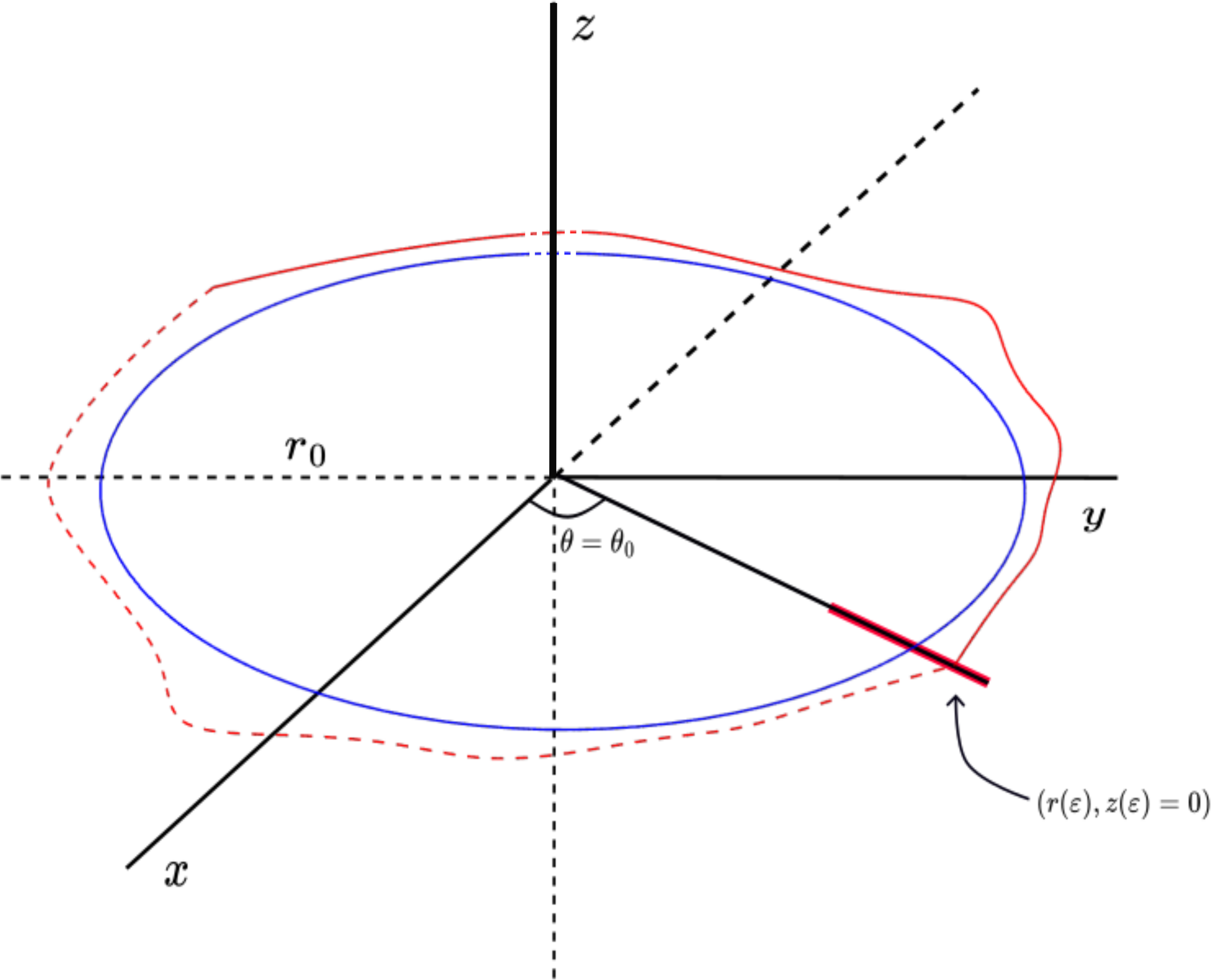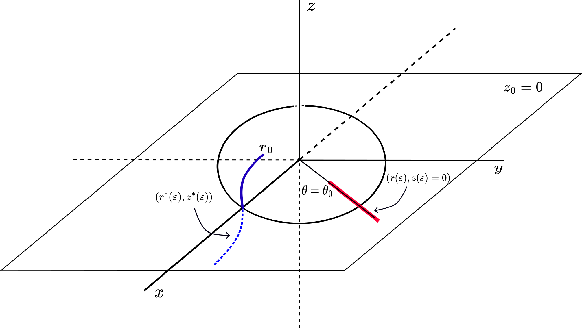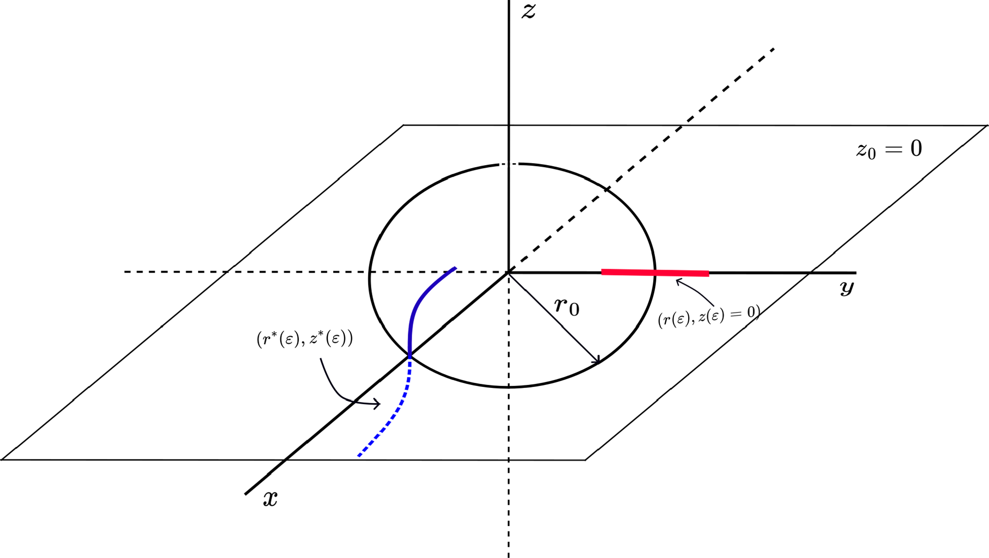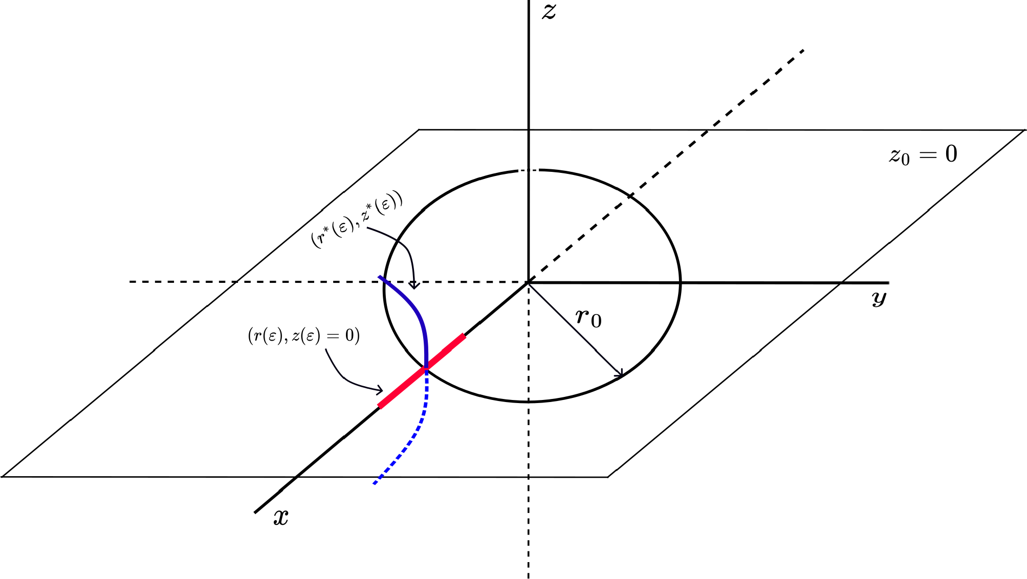



1 Introduction
The objective of this article is to demonstrate the existence of different families of reversible symmetric periodic solutions in close approximation to circular periodic solutions of some three-dimensional unperturbed ordinary differential equations (ODEs). In more precise terms, it is assumed that the ODEs are analytic and are symmetric with respect to some reversible symmetry, called S. That is, we consider the system
 $$ \begin{align} \dot{x}= X(x, \varepsilon), \end{align} $$
where
 $X: U \times \mathbb {R} \subset {\mathbb {R}}^3 \times \mathbb {R} \rightarrow {\mathbb {R}}^3$
(U is an open set of
 ${\mathbb {R}}^3$
) is an analytic function in both variables,
 $\varepsilon $
is assumed to be a small parameter. Let
 $S :{\mathbb {R}}^3 \rightarrow {\mathbb {R}}^3$
be a linear transformation in involution, that is,
 $S^2 = I$
. A vector field X is said S-reversible symmetric if
 $X \circ S = -S \circ X$
for all
 $x \in U$
, with
 $\varepsilon $
fixed; that is,
 $X(S x, \varepsilon )= -S(X(x, \varepsilon ))$
. Additionally, one solution
 $\mathbf {x}(t,\varepsilon )$
of the system (1) is called S-reversible symmetric if
 $\mathbf {x}(t,\varepsilon )= S(\mathbf {x}(-t,\varepsilon ))$
(see [Reference Moser21]).
In order to make this work self-contained, we recall the following basic but essential result for our purposes.
Lemma 1.1 Let
 $S: {\mathbb {R}}^3 \rightarrow {\mathbb {R}}^3$
be a reversible symmetry of the vector field (1). We denote the set of the fixed points of the symmetry S as
 $\mathscr {L}$
:=Fix
 $(S)=\{\xi \in {\mathbb {R}}^3: S(\xi )= \xi \}$
. Assume that
 $\mathbf {x}(t,\xi , \varepsilon )$
is solution of (1) such that:
-
1)
 $\xi \in \mathscr {L}$
,
-
2)
$\mathbf {x}(\tau /2,\xi , \varepsilon ) \in \mathscr {L}$
,


then
 $\mathbf {x}(t,\xi , \varepsilon )$
is a
 $\tau $
-periodic solution of (1). Moreover, this solution is S-reversible symmetric, that is,
 $\mathbf {x}(t)= S(\mathbf {x}(-t))$
.
The proof of this lemma can be found in [Reference Moser21].
The existence of periodic solutions has been the subject of study by many authors, who have employed a variety of approaches. It is important to recall the relevant literature on this topic, including the works of Poincaré [Reference Poincaré22], Hale [Reference Hale10, Reference Hale11], Farkas [Reference Farkas7], Sanders et al. [Reference Sanders, Verhulst and Murdock23], and Verhulst [Reference Verhulst24], among others. For example, in [Reference Duistermaat4], Duistermaat considers ODEs of the form
 $\dot {x} = f(t, x, \omega , \varepsilon )$
, with
 $x \in \mathbb {R}^n$
, where f is periodic in t with period
 $\omega $
. This study addresses the existence of periodic solutions as continuations of a known periodic solution of the unperturbed system
 $\dot {x} = f(t, x, \omega _0, \varepsilon _0)$
with initial condition
 $\xi _0$
. In another paper [Reference Duistermaat5], the same problem is considered, but under the assumption of the existence of a first integral. In both cases, the existence of periodic solutions is reduced to finding appropriate initial conditions
 $\xi $
of the unperturbed system, or equivalently, to solving the periodicity equation
 $\phi (\xi , \omega , \varepsilon ) = x(\omega , \xi , \omega , \varepsilon ) - \xi = 0$
. In this way, one obtains a periodic solution with initial condition
 $\xi $
and period
 $\omega $
. The authors study the case in which the rank of
 $D_{\xi } \phi (\omega _0, \xi _0, \omega _0, \varepsilon _0)$
is maximal. However, in the autonomous case, it is known that this rank is never maximal, and thus these results cannot be directly applied. The work [Reference Duistermaat5] also considers the case in which the dimension of
 $\ker D_{\xi } \phi (\omega _0, \xi _0, \omega _0, \varepsilon _0)$
is one. Lamb and Roberts [Reference Lamb and Roberts18] provide a comprehensive overview of the role of time-reversal symmetry in dynamical systems, with particular emphasis on its connections to Hamiltonian and equivariant structures. Their work surveys major developments in the theory of reversible systems, including symmetric periodic orbits, local bifurcations, homoclinic phenomena, and renormalization techniques. They also explore various contexts, both in physics and mathematics, where time-reversible dynamics naturally arise. The study includes an extensive bibliography, making it a valuable resource for further exploration of time-reversal symmetry in dynamical systems.
In this work, we present results aimed at obtaining reversible symmetric periodic solutions as a consequence of imposing symmetry on the vector field of the ODEs. In the Concluding Remarks section, we analyze each reversible symmetry considered in this article, comparing two different approaches: the method developed herein and the Averaging Method. We highlight the differences between these methods and discuss the type of information each provides regarding the existence of periodic solutions.
In this article, we consider the following family of ODEs in
 $\mathbb {R}^3$
of the form:
 $$ \begin{align} \begin{aligned} \dot{x}_1 & = -x_2 + \varepsilon^{\alpha} f_1(x_1,x_2,x_3) + \varepsilon^{\alpha+\ell} R_1(x_1,x_2,x_3, \varepsilon), \\[0.25pc] \dot{x}_2 & = \ \ x_1 + \varepsilon^{\alpha} g_1(x_1,x_2,x_3) + \varepsilon^{\alpha+\ell} R_2(x_1,x_2,x_3, \varepsilon),\\[0.25pc] \dot{x}_3 & = \varepsilon^{\alpha} h_1(x_1,x_2,x_3) + \varepsilon^{\alpha+\ell} R_3(x_1,x_2,x_3, \varepsilon), \end{aligned} \end{align} $$
where
 $\alpha , \ell \in \mathbb {N}$
. Here, the dot denotes the derivative with respect to the independent real variable t, and
 $\varepsilon $
is a small parameter. In these differential systems, the functions
 $f_1$
,
 $g_1$
,
 $h_1$
, and
 $R_i$
are analytic functions in the Cartesian variables, and moreover,
 $R_i$
are also analytic in
 $\varepsilon $
. As we will see throughout this article, these conditions can be weakened by requiring the functions to belong to the appropriate class
 $C^k$
. Of course, in the spatial case, the origin is an equilibrium point and
 ${\dim W^c(0,0,0) = 3}$
; in particular, for
 $\varepsilon = 0$
, the
 $xy$
-plane is foliated by periodic solutions of fixed period
 $2\pi $
.
There are many works in the literature that address the problem of symmetries and their implications in ODEs. In particular, we are interested in works concerning reversible or time-reversible symmetries, where conditions for the existence of symmetric periodic solutions are established.
For example, in [Reference Heinbockel and Struble13], the authors consider the system
 $\dot {x} = f(t, x)$
, where
 $x \in \mathbb {R}^n$
and f is T-periodic in t. It is assumed that
 $f(-t, Qx) = -Q f(t, x)$
for all t and x, for a certain constant matrix Q. In that work, the authors prove a simple theorem that characterizes the existence of periodic solutions of the system possessing the symmetry property induced by Q. This result is similar to that given in our Lemma 1.1. Moreover, in the two-dimensional case, periodic solutions are constructed using elementary geometrical and analytical arguments together with the presence of reversible symmetries.
In [Reference Fečkan, Rontó and Dilna8], the authors consider a nonlinear ODE of the form
 $\dot {x} = \varepsilon f(t, x)$
, where
 ${x \in \mathbb {R}^n}$
,
 $t \in \mathbb {R}$
, and
 $\varepsilon \in \mathbb {R}$
is a small parameter. It is assumed that f satisfies the following symmetry: there exist a matrix A and a function
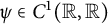 $\psi \in C^1(\mathbb {R}, \mathbb {R})$
such that
 $A f(t, x) = \psi '(t) f(\psi (t), A x)$
. For this class of weakly nonlinear ODEs, the authors prove the existence of a unique symmetric solution and provide information about its stability.
In [Reference Dilna and Fečkan3], the authors consider a nonlinear ODE of the form
 $\dot {x} = \varepsilon f(t, x, \mu )$
, where
 $x \in \mathbb {R}^n$
,
 $\mu \in \mathbb {R}^k$
,
 $t \in \mathbb {R}$
, and
 $\varepsilon \in \mathbb {R}$
is a small parameter. The symmetry condition assumed is
 $A f(t, x, \mu ) = -f(-t - \tau , A x, \mu )$
, where A is a constant matrix,
 $\tau \in \mathbb {R}$
is fixed, and f is
 $\tau $
-periodic in t. The authors establish two results about the existence of periodic symmetric solutions for this class of weakly nonlinear ODEs, under the assumption that the initial condition satisfies
 $x_0 \in \ker (I - A)$
. They analyze the cases when
 $\ker (I - A) = \{0\}$
and
 $\ker (I - A) \neq \{0\}$
, considering parametric dependence and time-reversal symmetries. Furthermore, they rigorously analyze the local asymptotic behavior of these solutions. It is worth noting that these previous works consider spatially non-autonomous ODEs, unlike the approach presented in this article.
In [Reference Knobloch and Vanderbauwhede17], the authors introduce a general reduction method to study periodic solutions near equilibrium points in autonomous reversible systems. They consider the autonomous differential equation
 $\dot {x} = f(x, \lambda )$
, where
 $f: \mathbb {R}^n \times \mathbb {R}^m \to \mathbb {R}^n$
is a smooth vector field satisfying
 $f(0, \lambda ) = 0$
for all
 $\lambda \in \mathbb {R}^m$
. For some
 $\lambda _0 \in \mathbb {R}^m$
, the linear operator
 $A_0 := D_x f(0, \lambda _0) \in \mathscr {L}(\mathbb {R}^n)$
is nonsingular. The system is assumed to be reversible, that is, there exists a linear involution
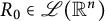 $R_0 \in \mathscr {L}(\mathbb {R}^n)$
(i.e.,
 $R_0^2 = I$
) such that
 $f(R_0 x, \lambda ) = -R_0 f(x, \lambda )$
. No restrictions are imposed on the linearization at the equilibrium, allowing for higher multiplicities and all types of resonances. The problem is reduced to one for a lower-dimensional system, which is either conservative or reversible and also possesses an additional symmetry. The proof combines normal forms and the Lyapunov–Schmidt reduction method.
There are also several studies in the literature where the proposed system undergoes a zero-Hopf bifurcation. Examples include predator–prey models and Chua’s system, a classical model in electronic circuits. Some references include [Reference Cardin and Llibre1, Reference Chen2, Reference Falconi, Vera-Damian and Vidal6, Reference Ginoux and Llibre9, Reference Han, Llibre and Tian12, Reference Huang and Wang15, Reference Li, Liu and Wei19, Reference Wang, Lu, Wang and Huang25]. In these works, the existence of periodic solutions is proven as a bifurcation from an equilibrium point with eigenvalues
 $\pm i$
and
 $0$
. The existence of such periodic solutions, typically with variable period, is often established using Averaging theory and cylindrical coordinates.
In our problem, the unperturbed system (2) also admits a zero-Hopf bifurcation, i.e., its linearization has eigenvalues
 $\pm i$
and
 $0$
. Therefore, the continuation of periodic solutions in the perturbed system is studied using symmetry conditions to obtain symmetric periodic solutions.
In [Reference Kassa, Llibre and Makhlouf16], Kassa, Llibre, and Makhlouf provide necessary and sufficient conditions for the existence of two or more limit cycles bifurcating from a zero-Hopf equilibrium in the following three-dimensional Lipschitzian differential system:
 $$ \begin{align} \dot{x} = y, \quad \dot{y} = z, \quad \dot{z} = -a|x| - y + 3y^3 - xz - b, \end{align} $$
when
 $a = b = 0$
. Although the system is not initially in the form of (2), the authors apply changes of coordinates and introduce a small parameter by setting
 $a = \varepsilon $
,
 $b = \varepsilon ^2 \beta $
, and rescaling
 $(x, y, z) = \varepsilon (X, Y, Z)$
. Then, they apply the transformation
 $(X, Y, Z) = (u + w, -v, -u)$
to rewrite the system in a form resembling ours. Finally, they use cylindrical coordinates and take
 $\theta $
as a new independent variable to compute the averaged function. By applying averaging theory, they prove the existence and uniqueness of a T-periodic solution based on the analysis of two equations. In contrast, our method often requires analyzing only one equation due to the presence of reversible symmetries.
The main objective of this article is to carry out an analytical study that provides sufficient conditions for the existence of several families of reversible symmetric periodic solutions of the spatial system (2), close to the circular solutions of the corresponding unperturbed differentiable system. We assume that the perturbed system (2) possesses a reversible symmetry, specifically reflections with respect to the coordinate axes or coordinate planes. More precisely, we aim to determine under which conditions the circular orbits of the system
 $$ \begin{align*}\dot{x}_1 = -x_2, \quad \dot{x}_2 = x_1, \quad \dot{x}_3 = 0 \end{align*} $$
can be continued as periodic orbits of the full system. To carry out our work, we introduce the change to cylindrical coordinates:
 $$ \begin{align*}x_1 = r \cos \theta, \quad x_2 = r \sin \theta, \quad x_3 = z, \end{align*} $$
then the system (2) takes the form
 $$ \begin{align} \begin{aligned} \dot{r} & = \varepsilon^{\alpha} \left[ \tilde{f}_1(r,\theta,z) \cos \theta + \tilde{g}_1(r,\theta,z) \sin \theta \right] + \mathcal{O}(\varepsilon^{\alpha+1}), \\ \dot{\theta} & = 1 + \frac{\varepsilon^\alpha}{r} \left[ \tilde{g}_1(r,\theta,z) \cos \theta - \tilde{f}_1(r,\theta,z) \sin \theta \right] + \mathcal{O}(\varepsilon^{\alpha+1}), \\ \dot{z} & = \varepsilon^\alpha \tilde{h}_1(r,\theta,z) + \mathcal{O}(\varepsilon^{\alpha+1}), \end{aligned} \end{align} $$
where
 $\tilde {f}_1(r,\theta ,z) = f_1(r \cos \theta , r \sin \theta , z)$
,
 $\tilde {g}_1(r,\theta ,z) = g_1(r \cos \theta , r \sin \theta , z)$
, and
 $\tilde {h}_1(r,\theta ,z) = h_1(r \cos \theta , r \sin \theta , z)$
.
We write the previous system in the reduced form:
 $$ \begin{align} \begin{aligned} \dot{r} & = \varepsilon^{\alpha} F_1(r,\theta,z) + \mathcal{O}(\varepsilon^{\alpha+1}), \\ \dot{\theta} & = 1 + \varepsilon^\alpha G_1(r,\theta,z) + \mathcal{O}(\varepsilon^{\alpha+1}), \\ \dot{z} & = \varepsilon^\alpha K_1(r,\theta,z) + \mathcal{O}(\varepsilon^{\alpha+1}), \end{aligned} \end{align} $$
where the functions
 $F_1$
,
 $G_1$
, and
 $K_1$
are given by
 $$ \begin{align} \begin{aligned} F_1(r,\theta,z) & = \tilde{f}_1(r,\theta,z) \cos \theta + \tilde{g}_1(r,\theta,z) \sin \theta, \\ G_1(r,\theta,z) & = \frac{1}{r} \left[ \tilde{g}_1(r,\theta,z) \cos \theta - \tilde{f}_1(r,\theta,z) \sin \theta \right], \\ K_1(r,\theta,z) & = \tilde{h}_1(r,\theta,z). \end{aligned} \end{align} $$
Remark 1. For simplicity, and to avoid complications arising from a possible singularity at
 $r = 0$
in system (5), we consider only the case where
 $r> 0$
.
We are now ready to state our first result for the spatial case, which provides sufficient conditions for the existence of
 $T_j$
-reversible symmetric periodic solutions of (5), both with fixed period
 $2\pi $
and with a period close to
 $2\pi $
(but not necessarily fixed). We consider reversible symmetries such that one maps
 $x_1 \mapsto -x_1$
and the other maps
 $x_2 \mapsto -x_2$
.
Theorem 1.1 (
$T_j$
-reversible symmetric periodic solutions)

Let
 $\delta _1 = 1$
and
 $\delta _2 = 0$
. Assume that the system (2) admits a reversible symmetry of the form:
 $$\begin{align*}T_j(x_1, x_2, x_3) = \left( (-1)^j x_1,\ (-1)^{j+1} x_2,\ x_3 \right), \quad j = 1,2. \end{align*}$$
Let
 $(r_0(t), \theta _0(t), z_0(t)) = \left ( r_0 + \delta r,\ t + \delta _j \frac {\pi }{2},\ z_0 + \delta z \right )$
be a
 $T_j$
-symmetric and
 $2\pi $
-periodic solution of the unperturbed system (5), of radius
 $r_0 + \delta r$
and lying in the plane
 $z = z_0 + \delta z$
with
 $\delta r$
and
 $\delta z$
sufficiently small. Suppose that there exist
 $r_0$
and
 $z_0$
such that the following conditions are satisfied:
-
a)
$\displaystyle \int _0^\pi \left [ \tilde {g}_1\left (r_0, s + \delta _j \frac {\pi }{2}, z_0\right ) \cos \left (s + \delta _j \frac {\pi }{2}\right ) - \tilde {f}_1\left (r_0, s + \delta _j \frac {\pi }{2}, z_0\!\right ) \!\sin \!\left (s + \delta _j \frac {\pi }{2}\!\right )\! \right ] ds {=} 0$
, -
b)
$\displaystyle \int _0^\pi\! \left [ \!\frac {\partial \tilde {g}_1}{\partial r} \!\left (\!r_0, s + \delta _j \frac {\pi }{2}, z_0\!\right ) \!\cos \!\left (\!s + \delta _j \frac {\pi }{2}\!\right )\! - \!\frac {\partial \tilde {f}_1}{\partial r} \!\left (\!r_0, s + \delta _j \frac {\pi }{2}, z_0\!\right ) \!\sin \!\left (\!s + \delta _j \frac {\pi }{2}\!\right ) \right ]\! ds \neq 0$
, -
c)
$\displaystyle \int _0^\pi \!\left [\! \frac {\partial \tilde {g}_1}{\partial z} \left (\!r_0, s \!+\! \delta _j \frac {\pi }{2}, z_0\!\right )\! \cos\! \left (s\! +\! \delta _j \frac {\pi }{2}\!\right )\! - \!\frac {\partial \tilde {f}_1}{\partial z} \!\left (r_0, s + \delta _j \frac {\pi }{2}, z_0\right ) \sin \left (s + \delta _j \frac {\pi }{2}\!\right ) \!\right ]\! ds \!\neq\! 0$
.



Then, the following holds:
-
i) (Fixed period and two parameters
$(\delta z, \varepsilon )$
) If conditions a) and b) hold for
$j = 1$
or
$j = 2$
, and
$\varepsilon $
is sufficiently small, then there exists a unique family of initial conditions
$ (r(\varepsilon ), \theta (\varepsilon ), z(\varepsilon )) = \left ( r_0 + \delta r(\delta z, \varepsilon ),\ \delta _j \frac {\pi }{2},\ z_0 + \delta z \right )$
, depending on two parameters, with
$\delta r(0,0) = 0$
, such that each of them defines a family of
$T_j$
-reversible symmetric periodic solutions (for
$j=1$
or
$j=2$
) of the full system (2) with fixed period
$T = 2\pi $
. Moreover, these solutions are close to the circular solution of radius
$r_0$
and near the plane
$z = z_0$
. -
ii) (Fixed period and two parameters
$(\delta r, \varepsilon )$
) If conditions a) and c) hold for
$j = 1$
or
$j = 2$
, and
$\delta r$
and
$\varepsilon $
are sufficiently small, then there exists a unique family of initial conditions
$(r(\varepsilon ), \theta (\varepsilon ), z(\varepsilon )) = \left ( r_0 + \delta r,\ \delta _j \frac {\pi }{2},\ z_0 + \delta z(\delta r, \varepsilon ) \right )$
, depending on two parameters, with
$\delta z(0,0) = 0$
, such that each of them defines a family of
$T_j$
-reversible symmetric periodic solutions (for
$j=1$
or
$j=2$
) of the full system (2) with fixed period
$T = 2\pi $
. Moreover, these solutions are close to the circular solution of radius
$r_0$
and near the plane
$z = z_0$
. -
iii) (Variable period and three parameters
$(\delta r, \delta z, \varepsilon )$
) If condition a) holds for
$j = 1$
or
$j = 2$
, and
$\delta r$
,
$\delta z$
, and
$\varepsilon $
are sufficiently small, then there exists a unique differentiable function
$\tau (\delta r, \delta z, \varepsilon )$
with
$\tau (0,0,0) = \pi $
, such that each initial condition
$(r_0 + \delta r,\ \delta _j \frac {\pi }{2},\ z_0 + \delta z)$
defines a family of
$T_j$
-reversible symmetric periodic solutions of the full system (2), depending on three parameters
$(\delta r, \delta z, \varepsilon )$
, with period close to
$2 \tau (\delta r, \delta z, \varepsilon ) = 2\pi + \mathcal {O}(\varepsilon ^\alpha )$
. Moreover, these solutions are close to the circular solution of radius
$r_0$
and near the plane
$z = z_0$
.















Furthermore, the characteristic multipliers of the
 $T_1$
-symmetric and
 $T_2$
-symmetric periodic solutions
 $\varphi (t, (r(\varepsilon ), \theta (\varepsilon ), z(\varepsilon )), \varepsilon )$
are, respectively
 $ 1,\ 1 + \varepsilon ^\alpha \lambda _1 +\mathcal {O}(\varepsilon ^{\alpha +1}),\ 1 + \varepsilon ^\alpha \lambda _2 + \mathcal {O}(\varepsilon ^{\alpha +1})$
and
 $ 1,\ 1 + \varepsilon ^\alpha \lambda _3 +\mathcal {O}(\varepsilon ^{\alpha +1}),\ 1 + \varepsilon ^\alpha \lambda _4 + \mathcal {O}(\varepsilon ^{\alpha +1})$
.
In Section 2, we present the proof of this theorem. Note that the conditions of the previous theorem involve only the functions
 $f_1$
and
 $g_1$
, however,
 $h_1$
must have the reversible symmetry condition. We include in Theorem 1.1 case
 $iii)$
, that is, the existence of periodic solutions with a period close to
 $2\pi $
but not fixed, because it requires fewer restrictions. Our second result assumes the existence of the reversible symmetry
 $T_3(x_1,x_2,x_3)= (x_1,x_2,-x_3)$
, that is, reflection with respect to the plane
 $x_1x_2$
.
Theorem 1.2 (
$T_3$
-reversible symmetric periodic solutions)

Assume that the system (2) possesses the reversible symmetry
 $\displaystyle T_3(x_1,x_2,x_3)= (x_1,x_2,-x_3)$
. Let
 $\displaystyle (r_0(t),\theta _0(t),z_0(t))=(r_0+ \delta r, t+ \theta _0, 0)$
(with
 $\theta _0 \in [0,2\pi )$
fixed) be a
 $T_3$
-symmetric and
 $2\pi $
-periodic solution of the unperturbed system in (5), of radius
 $r_0 + \delta r$
with
 $\delta r$
sufficiently small, and lying on the plane
 $z = 0$
. Assume that there exist
 $(r_0, \theta _0)$
such that the following conditions are satisfied:
-
a)
$\displaystyle \int _0^\pi \tilde {h}_1(r_0, s+\theta _0, 0) \, ds = 0$
; -
b)
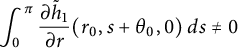
$\displaystyle \int _0^\pi \frac {\partial \tilde {h}_1}{\partial r}(r_0, s+\theta _0, 0) \, ds \neq 0$
; -
c)
$\tilde {h}_1(r_0, \pi +\theta _0, 0) \neq 0$
.


We have the following:
-
i) (Fixed period and one parameter
$\varepsilon $
) If conditions a) and b) hold and
$\varepsilon $
is sufficiently small, then there exists a unique family of initial conditions
$\displaystyle (r(\varepsilon ), \theta (\varepsilon ), z(\varepsilon )) = (r_0 + \delta r(\varepsilon ), \theta _0, 0)$
depending on one parameter, with
$\delta r(0) = 0$
, such that each of them generates a family of
$T_3$
-reversible symmetric periodic solutions of the complete system (2) with fixed period
$T = 2\pi $
. Moreover, these solutions are close to the circular solution of radius
$r_0$
and near the plane
$z = 0$
. -
ii) (Variable period and two parameters
$(\delta r, \varepsilon )$
) If conditions a) and c) hold and both
$\delta r$
and
$\varepsilon $
are sufficiently small, then there exists a unique differentiable function
$\tau (\delta r, \varepsilon )$
with
$\tau (0,0) = \pi $
, such that any initial condition
$(r_0 + \delta r, \theta _0, 0)$
generates a family of
$T_3$
-reversible symmetric periodic solutions of the complete system (2), depending on the two parameters
$(\delta r, \varepsilon )$
, with period close to
$2\tau (\delta r, \varepsilon ) = 2\pi + \mathcal {O}(\varepsilon ^\alpha )$
. Moreover, they are close to a circular solution of radius
$r_0$
and near the plane
$z = 0$
.











Furthermore, the characteristic multipliers of the periodic solution
 $\displaystyle \varphi (t, (r(\varepsilon ), \theta (\varepsilon ), z(\varepsilon )), \varepsilon )$
are
 $1, 1 + \varepsilon ^\alpha \lambda _1 + \mathcal {O}(\varepsilon ^{\alpha +1}), 1 + \varepsilon ^\alpha \lambda _2 + \mathcal {O}(\varepsilon ^{\alpha +1})$
.
Note that in the above theorem, the conditions involve only the function
 $h_1$
. Figure 1 shows the existence of the curve of initial conditions that give rise
 $T_3$
-reversible symmetric periodic solution of period fixed close to
 $2\pi $
and it is on the
 $z=0$
plane.




The next result concerns another type of reversible symmetry that changes two variables.
Theorem 1.3 (
$T_{j+4}$
-reversible symmetric periodic solutions)

Let
 $\delta _1 = 1$
and
 $\delta _2 = 0$
. Assume that the system (2) admits the reversible symmetry
 $$\begin{align*}T_{j+4}(x_1,x_2,x_3) = ((-1)^j x_1, (-1)^{j+1} x_2, -x_3), \quad j=1,2. \end{align*}$$
Let
 $(r_0(t), \theta _0(t), z_0(t)) = (r_0 + \delta r, t + \delta _j \frac {\pi }{2}, \delta z)$
be a
 $2\pi $
-periodic solution of the unperturbed system in (5) with
 $\delta r$
and
 $\delta z$
sufficiently small. Suppose that there exists
 $r_0> 0$
such that the following conditions are satisfied:
-
a)
$\displaystyle \int _0^{\pi } \tilde {h}_1\left (r_0, s + \delta _j \frac {\pi }{2}, 0\right ) \, ds = 0$
, -
b)
$\displaystyle \int _0^{\pi } \frac {\partial \tilde {h}_1}{\partial r} \left (r_0, s + \delta _j \frac {\pi }{2}, 0\right ) \, ds - \tilde {h}_1\left (r_0, \pi + \delta _j \frac {\pi }{2}, 0\right ) \cdot I \neq 0$
,


where
 $$\begin{align*}I = \int_0^{\pi} \left[ \frac{\partial \tilde{g}_1}{\partial r} \left(r_0, s + \delta_j \frac{\pi}{2}, 0\right) \cos \left(s + \delta_j \frac{\pi}{2} \right) - \frac{\partial \tilde{f}_1}{\partial r} \left(r_0, s + \delta_j \frac{\pi}{2}, 0\right) \sin \left(s + \delta_j \frac{\pi}{2} \!\right) \!\right] \ ds. \end{align*}$$
If conditions a) and b) are satisfied, and
 $\delta r$
and
 $\varepsilon $
are sufficiently small, then there exists a unique one-parameter family of initial conditions
 $(r_0+\delta r(\varepsilon ), \delta _j \frac {\pi }{2}, 0)$
, with
 $\delta r(0) = 0$
, and a differentiable function
 $\tau (\varepsilon )$
, such that each of them gives rise to a
 $T_{j+4}$
-reversible symmetric periodic solution of the complete system (2) with period
 $2\tau (\varepsilon ) = 2\pi + \mathcal {O}(\varepsilon ^\alpha )$
. Moreover, these solutions are close to a circular solution of radius
 $r_0$
and lie on the
 $x_1x_2$
-plane.
The proof of this result can be found in Section 4. Observe that the above theorem involves the functions
 $f_1$
,
 $g_1$
, and
 $h_1$
. Furthermore, we only obtained periodic solutions with variable period.
2 Proof of Theorem 1.1
Consider the system in
 $\mathbb {R}^3$
given by (2), and assume that it is
 $T_j$
-reversible symmetric for
 $j=1$
or
 $j=2$
. Note that when
 $j=1$
, the symmetry
 $T_1$
is a reflection with respect to the
 $x_2x_3$
-plane, and when
 $j=2$
,
 $T_2$
is a reflection with respect to the
 $x_1x_3$
-plane. The set of fixed points for
 $j=1$
or
 $j=2$
is given by
 $\mathcal {L}_j := \text {Fix}(T_j) = \{(x_1,x_2,x_3) \in \mathbb {R}^3 : x_j = 0\}$
. In this case, we have that
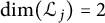 $\dim (\mathcal {L}_j) = 2$
.
From the reversible symmetry condition, we have that for
 $j=1$
,
 $$ \begin{align*} f_1(-x_1, x_2, x_3) &= f_1(x_1,x_2,x_3), \ g_1(-x_1, x_2, x_3) = -g_1(x_1,x_2,x_3), \ h_1(-x_1, x_2, x_3)\\& = -h_1(x_1,x_2,x_3), \end{align*} $$
that is, the functions
 $g_1$
and
 $h_1$
are odd in the variable
 $x_1$
, and
 $f_1$
is even in
 $x_1$
. For
 $j=2$
, we obtain
 $$ \begin{align*} \begin{aligned} f_1(x_1, -x_2, x_3) &= -f_1(x_1,x_2,x_3), \ g_1(x_1, -x_2, x_3) = g_1(x_1,x_2,x_3), \ h_1(x_1, -x_2, x_3)\\& = -h_1(x_1,x_2,x_3), \end{aligned} \end{align*} $$
that is, the functions
 $f_1$
and
 $h_1$
are odd in
 $x_2$
, and
 $g_1$
is even in
 $x_2$
.
Our next step is to obtain an approximation of the solutions of the perturbed system (5). For this, we suppose the solution has the form:
 $$ \begin{align} \begin{aligned} r(t,\varepsilon) &= r_0(t)+ \varepsilon^{\alpha} r_1(t)+\mathcal{O}(\varepsilon^{\alpha+1}), \\ \theta(t,\varepsilon) &= \theta_0(t)+ \varepsilon^{\alpha} \theta_1(t)+\mathcal{O}(\varepsilon^{\alpha+1}), \\ z(t,\varepsilon) &= z_0(t)+ \varepsilon^{\alpha} z_1(t)+\mathcal{O}(\varepsilon^{\alpha+1}). \end{aligned} \end{align} $$
It can be verified that the variational equations in this case are
 $$ \begin{align} \begin{aligned} \dot{r}_0 &= 0, \\ \dot{\theta}_0 &= 1, \\ \dot{z}_0 &= 0, \\ \dot{r}_1 &= F_1(r_0(t),\theta_0(t),z_0(t)), \\ \dot{\theta}_1 &= G_1(r_0(t),\theta_0(t),z_0(t)), \\ \dot{z}_1 &= K_1(r_0(t),\theta_0(t),z_0(t)). \end{aligned} \end{align} $$
Considering that the initial condition of the solution is of the form
 $(r_0, \theta _0, z_0)$
, and solving the equations in (8), we obtain
 $$ \begin{align} \begin{aligned} r_0(t) &= r_0, \\ \theta_0(t) &= t + \theta_0, \\ z_0(t) &= z_0, \\ r_1(t) &= \int_0^t \left[ \tilde{f}_1(r_0,s+\theta_0,z_0)\cos (s+\theta_0) + \tilde{g}_1(r_0,s+\theta_0,z_0)\sin (s+\theta_0) \right] ds, \\ \theta_1(t) &= \frac{1}{r_0} \int_0^t \left[ \tilde{g}_1(r_0,s+\theta_0,z_0) \cos (s+\theta_0)- \tilde{f}_1(r_0,s+\theta_0,z_0) \sin (s+\theta_0) \right] ds, \\ z_1(t) &= \int_0^t \tilde{h}_1(r_0,s+\theta_0,z_0)\, ds. \end{aligned} \end{align} $$
The characterization of the points in the set
 $\mathcal {L}_j$
in cylindrical coordinates is given by
 $\theta = \delta _j \frac {\pi }{2} \ (\text {mod } \pi )$
for
 $j=1,2$
, respectively, for each symmetry
 $T_1$
and
 $T_2$
. Thus, the solution of the unperturbed system has the form
 $(r_0(t), \theta _0(t), z_0(t)) = (r_0, t + \delta _j \frac {\pi }{2}, z_0)$
, with initial condition
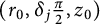 $(r_0, \delta _j \frac {\pi }{2}, z_0)$
, and it is a
 $2\pi $
-periodic circular solution of radius
 $r_0$
on the plane
 $z = z_0$
, with
 $(r_0, \delta _j \frac {\pi }{2}, z_0) \in \mathcal {L}_j$
for
 $j = 1,2$
.
Lemma 2.1 Let
 $j=1$
or
 $j=2$
such that
 $\delta _1=1$
and
 $\delta _2=0$
.
A solution
 $(r(t, (r_0,\theta _0,z_0),\varepsilon ),\theta (t,(r_0,\theta _0,z_0),\varepsilon ),z(t,(r_0,\theta _0,z_0),\varepsilon ))$
of the perturbed system (4) is
 $2\pi $
-periodic and
 $T_j$
-reversible (
 $j=1$
or
 $j=2$
) symmetric if we take
 $\theta _0= \delta _j \frac {\pi }{2}$
and it satisfies the condition
 $$\begin{align*}\theta(\pi,(r_0,\delta_j \tfrac{\pi}{2},z_0),\varepsilon)=\delta_j \tfrac{\pi}{2} \ (\textit{mod} \ \pi), \end{align*}$$
where
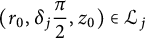 $\displaystyle (r_0,\delta _j \frac {\pi }{2},z_0) \in \mathcal {L}_j$
is the initial condition.
Now, from Lemma 2.1, since
 $\theta _0(\pi ) = \pi + \delta _j \tfrac {\pi }{2}$
, the first-order approximation
 $\theta _1(t,(r_0,\theta _0,z_0))$
at
 $t=\pi $
takes the form:
 $$ \begin{align*} \theta_1\left(\pi,\left(r_0,\delta_j \tfrac{\pi}{2},z_0\right)\right) &= \frac{1}{r_0} \int_0^\pi \left[ \tilde{g}_1\left(r_0,s+\delta_j \tfrac{\pi}{2},z_0\right) \cos\left(s+\delta_j \tfrac{\pi}{2}\right)\right.\\&\quad \left. - \tilde{f}_1\left(r_0,s+\delta_j \tfrac{\pi}{2},z_0\right) \sin\left(s+\delta_j \tfrac{\pi}{2}\right) \right] ds, \end{align*} $$
then, the symmetry condition from Lemma 2.1 takes the form:
 $$ \begin{align} \theta\left(\pi,\left(r_0,\delta_j \tfrac{\pi}{2},z_0\right),\varepsilon\right) & = \pi + \delta_j \tfrac{\pi}{2} + \frac{\varepsilon^\alpha}{r_0} \displaystyle \int_0^{\pi} \left[ \tilde{g}_1\left(r_0,s +\delta_j \tfrac{\pi}{2},z_0\right) \cos\left(s+\delta_j \tfrac{\pi}{2}\right) \right.\nonumber \\ &\quad \!\left. - \tilde{f}_1\left(r_0,s+\delta_j \tfrac{\pi}{2},z_0\right) \sin\left(s+\delta_j \tfrac{\pi}{2}\right) \right] ds+ \mathcal{O}(\varepsilon^{\alpha+1}). \end{align} $$
Since
 $\theta (\pi ,(r_0,\delta _j \tfrac {\pi }{2},z_0),\varepsilon ) = \delta _j \tfrac {\pi }{2} \ (\textit {mod} \ \pi )$
, we consider
 $$\begin{align*}\theta\left(\pi,\left(r_0,\delta_j \tfrac{\pi}{2},z_0\right),\varepsilon\right) = \pi + \delta_j \tfrac{\pi}{2}, \end{align*}$$
so equation (10) is equivalent to solving
 $$ \begin{align} &\int_0^\pi \left[ \tilde{g}_1\left(r_0,s+\delta_j \tfrac{\pi}{2},z_0\right)\cos\left(s+\delta_j \tfrac{\pi}{2}\right) \right.\nonumber\\&\qquad \left.- \tilde{f}_1\left(r_0,s+\delta_j \tfrac{\pi}{2},z_0\right)\sin\left(s+\delta_j \tfrac{\pi}{2}\right) \right]ds + \mathcal{O}(\varepsilon) = 0. \end{align} $$
To obtain families of
 $T_j$
-reversible symmetric periodic solutions of fixed period
 $T = 2\pi $
(or variable period close to
 $2\pi $
), we perturb the initial condition by replacing
 $r_0$
and
 $z_0$
with
 $r_0 + \delta r$
and
 $z_0 + \delta z$
, respectively, where
 $\delta r$
and
 $\delta z$
are small. Clearly, for
 $j=1$
or
 $j=2$
, we have
 $(r_0+ \delta r, \delta _j \tfrac {\pi }{2}, z_0+ \delta z) \in \mathcal {L}_j$
. Thus, the initial radius and height of the
 $T_j$
-symmetric circular solution are now
 $r_0 + \delta r$
and
 $z_0 + \delta z$
, respectively. For future computations, we introduce time
 $\tau $
as an additional independent variable. Then, equation (10) becomes
 $$ \begin{align} \mathcal{F}(\tau,\delta r, \delta z, \varepsilon) & = \tau - \pi+ \frac{\varepsilon^{\alpha}}{r_0 + \delta r} \displaystyle \int_0^{\tau} \left[ \tilde{g}_1\left(r_0+\delta r,s +\delta_j \tfrac{\pi}{2},z_0+\delta z\right) \cos \left(s+\delta_j \tfrac{\pi}{2}\right) \right.\nonumber \\ &\quad \left.\! - \tilde{f}_1\left(r_0+\delta r,s +\delta_j \tfrac{\pi}{2},z_0+\delta z\right) \sin \left(s+\delta_j \tfrac{\pi}{2}\right) \right] ds, \end{align} $$
for
 $\varepsilon \neq 0$
, with
 $\mathcal {F}:\mathbb {R} \times \mathbb {R} \times \mathbb {R} \times \mathbb {R} \rightarrow \mathbb {R}$
.
In the case of a fixed period, we set
 $\tau = \pi $
, and then we define a new function on the three variables
 $(\delta r, \delta z, \varepsilon )$
as
 $$ \begin{align*} \overline{\mathcal{F}}(\delta r, \delta z, \varepsilon) & = \int_0^{\pi} \left[ \tilde{g}_1\left(r_0+\delta r,s+\delta_j \tfrac{\pi}{2},z_0+\delta z\right) \cos\left(s+\delta_j \tfrac{\pi}{2}\right)\right.\\&\quad \left.\! - \tilde{f}_1\left(r_0+\delta r,s+\delta_j \tfrac{\pi}{2},z_0+\delta z\right)\sin\left(s+\delta_j \tfrac{\pi}{2}\right) \right]ds,\end{align*} $$
with
 $\overline {\mathcal {F}}: \mathbb {R} \times \mathbb {R} \times \mathbb {R} \rightarrow \mathbb {R}$
.
Note that under hypothesis (a), we have
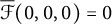 $\overline {\mathcal {F}}(0,0,0) = 0$
, since
 $\mathcal {F}(0,0,0,0) = 0$
. To prove item (i), we compute the derivative:
 $$ \begin{align*} \frac{\partial \overline{\mathcal{F}}}{\partial \delta r} (\delta r, \delta z, \varepsilon) &= \int_0^{\pi} \left[ \frac{\partial \tilde{g}_1}{\partial r}\left(r_0+\delta r,s+ \delta_j \tfrac{\pi}{2},z_0+\delta z\right) \cos\left(s+\delta_j \tfrac{\pi}{2}\right)\right.\\&\quad \left.\! - \frac{\partial \tilde{f}_1}{\partial r}\left(r_0+\delta r,s+ \delta_j \tfrac{\pi}{2},z_0+\delta z\right) \sin\left(s+\delta_j \tfrac{\pi}{2}\right) \right]ds. \end{align*} $$
Evaluating at
 $\delta r = 0$
,
 $\delta z = 0$
, and
 $\varepsilon = 0$
, hypothesis (b) implies that
 $$\begin{align*}\frac{\partial \overline{\mathcal{F}}}{\partial \delta r}(0,0,0) \neq 0, \end{align*}$$
and the Implicit Function Theorem ensures the result of item (i). The proof of item (ii) is analogous, taking the derivative with respect to
 $\delta z$
and using hypothesis (c).
To obtain
 $T_j$
-reversible symmetric periodic solutions (for
 $j=1$
or
 $j=2$
) of variable period close to
 $T = 2\pi $
, we treat time
 $\tau $
as an independent variable. Then, it is enough to observe that
 $$\begin{align*}\frac{\partial \mathcal{F}}{\partial \tau}(\pi, 0, 0, 0) = 1, \end{align*}$$
and by the Implicit Function Theorem, item (iii) follows.
In order to compute the characteristic multiplier associated with the family of periodic solutions
 $\varphi (t, (r_0+\delta r,\delta _j \frac {\pi }{2},z_0+\delta z),\varepsilon ) = (r(t,(r_0+\delta r,\delta _j \frac {\pi }{2},z_0+\delta z), \varepsilon ), \theta (t,(r_0+\delta r,\delta _j \frac {\pi }{2},z_0+\delta z), \varepsilon ), z(t,(r_0+\delta r,\delta _j \frac {\pi }{2},z_0+\delta z), \varepsilon ))$
obtained previously, we consider the cross section
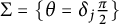 $\Sigma = \{ \theta = \delta _j \frac {\pi }{2} \}$
for the system (5). Thus, to study the stability of the
 $T(\varepsilon )$
-periodic solutions
 $\varphi (t, (r_0+\delta r,\delta _j \frac {\pi }{2},z_0+\delta z), \varepsilon )$
by means of the Poincaré map, we take this cross section as the domain of the return map. We take the map as
 $$\begin{align*}P : \Sigma \rightarrow \Sigma, \quad (r,z) \mapsto P(T(\varepsilon), r, z,\varepsilon)=P_\varepsilon(T(\varepsilon), r, z), \end{align*}$$
where
 $T(\varepsilon ) = 2\pi + \mathcal {O}(\varepsilon )$
. Since
 $$ \begin{align} r(T(\varepsilon), (r,\delta_j \tfrac{\pi}{2}, z), \varepsilon) &= r + \varepsilon^{\alpha} r_1(T(\varepsilon), (r,\delta_j \tfrac{\pi}{2}, z)) + \mathcal{O}(\varepsilon^{\alpha+1}), \end{align} $$
 $$ \begin{align} z(T(\varepsilon), (r,\delta_j \tfrac{\pi}{2}, z), \varepsilon) &= z + \varepsilon^{\alpha} z_1(T(\varepsilon), (r,\delta_j \tfrac{\pi}{2}, z)) + \mathcal{O}(\varepsilon^{\alpha+1}), \end{align} $$
the Poincaré map is
 $$\begin{align*}P_\varepsilon(r,z) = (r,z) + \varepsilon^{\alpha} \left( r_1(T(\varepsilon), (r,\delta_j \tfrac{\pi}{2}, z)), z_1(T(\varepsilon), (r,\delta_j \tfrac{\pi}{2}, z)) \right) + \mathcal{O}(\varepsilon^{\alpha+1}). \end{align*}$$
The derivative of
 $P_\varepsilon $
is
 $$\begin{align*}D_{(r,z)}P_\varepsilon(r,z) = \mathcal{I} + \varepsilon^{\alpha} A_j + \mathcal{O}(\varepsilon^{\alpha+1}), \end{align*}$$
where
 $$ \begin{align*}{\tiny A_j = \begin{pmatrix} \displaystyle\int_0^{2 \pi}\left[\frac{\partial \tilde{f}_1}{\partial r} \cos \left(s+\delta_j \frac{\pi}{2}\right)+ \frac{\partial \tilde{g}_1}{\partial r} \sin \left(s+\delta_j \frac{\pi}{2}\right)\right] ds & \displaystyle\int_0^{2 \pi}\left[\frac{\partial \tilde{f}_1}{\partial z} \cos \left(s+\delta_j \frac{\pi}{2}\right)+ \frac{\partial \tilde{g}_1}{\partial z} \sin \left(s+\delta_j \frac{\pi}{2}\right)\right] ds \\ \displaystyle\int_0^{2 \pi} \frac{\partial \tilde{h}_1}{\partial r} ds & \displaystyle\int_0^{2 \pi} \frac{\partial \tilde{h}_1}{\partial z} ds \end{pmatrix},} \end{align*} $$
and each function in the integrands is evaluated at the initial conditions
 $(r_0,s+\delta _j \frac {\pi }{2},z_0)$
for
 $j=1$
or
 $j=2$
. For the symmetry
 $T_2$
, the integrands of the integrals in the matrix
 $A_2$
are odd in s, so
 $A_2$
is the zero matrix when evaluated at
 $\delta r= 0$
,
 $\delta z= 0,$
and
 $\varepsilon =0$
and the derivate of
 $P_\varepsilon $
is
 $$\begin{align*}D_{(r,z)}P_\varepsilon(r,z) = \mathcal{I} + \mathcal{O}(\varepsilon^{\alpha+1}), \end{align*}$$
which applies to all families of
 $T_2$
-symmetric periodic solutions in items (i)–(iii).
However, for
 $T_1$
, the parity of
 $\tilde {f}_1$
,
 $\tilde {g}_1$
, and
 $\tilde {h}_1$
with respect to s cannot be determined, so the matrix
 $A_1$
may have nonzero entries. Therefore, the characteristic multipliers (i.e., eigenvalues of
 $D P_\varepsilon $
) can be calculated and may provide information about the stability of the associated symmetric periodic solution. This concludes the proof of Theorem 1.1.
Remark 2. The eigenvalues of the first approximation do not provide any information about the stability of the symmetric periodic solutions for any arbitrary functions possessing the
 $T_2$
-reversible symmetry.
We present the following example where we study the symmetry
 $T_1$
.
Example 2.1. Consider the system (2) with the following functions:
 $$ \begin{align} \begin{aligned} f_1(x_1,x_2,x_3)&= a_{200} x_1^2 + a_{210} x_1^2 x_2 + a_{201} x_1^2 x_3 + a_{012} x_2 x_3^2 + a_{030} x_2^3 + a_{400} x_1^4, \\ g_1(x_1,x_2,x_3)&= b_{101} x_1 x_3 + b_{300} x_1^3 + b_{120} x_1 x_2^2, \\ h_1(x_1,x_2,x_3)&= c_{110} x_1 x_2 + c_{101} x_1 x_3+c_{301} x^3 z, \end{aligned} \end{align} $$
where
 $a_{ij}, b_{ij}$
, and
 $c_{ij}$
are arbitrary real numbers, and
 $R_1,R_2$
, and
 $R_3$
arbitrary functions that have the reversible symmetry
 $T_1$
. Clearly, this system is
 $T_1$
-reversible. The previous functions (15) in cylindrical coordinates take the form as follows:
 $$ \begin{align*} \tilde{f}_1(r,\theta, z) &= a_{200} r^2 \cos ^2 \theta + a_{210} r^3 \sin \theta \cos ^2 \theta + a_{201} r^2 z \cos ^2 \theta\\&\quad + a_{012} r z^2 \sin \theta + a_{030} r^3 \sin ^3 \theta + a_{400} r^4 \cos ^4 \theta, \\ \tilde{g}_1(r,\theta, z) &= b_{101} r z \cos \theta + b_{300} r^3 \cos ^3 \theta + b_{120} r^3 \sin ^2 \theta \cos \theta , \\ \tilde{h}_1(r,\theta, z) &= c_{110} r^2 \sin \theta \cos \theta + c_{101} r z \cos \theta + c_{301} r^3 z \cos ^3 \theta. \end{align*} $$
We note that the equation in item a) of Theorem 1.1 reduces to
 $$ \begin{align} \displaystyle &\int_0^{\pi} \left[\tilde{g}_1\left(r_0,s+\frac{\pi}{2}, z_0\right) \sin s + \tilde{f}_1\left(r_0, s + \frac{\pi}{2},z_0\right) \cos s \right] d s\nonumber\\&\qquad = - \frac{4}{15} r^2 \left(5 a_{200}+5 a_{201} z+4 a_{400} r^2\right)=0. \end{align} $$
So, to apply item i) of Theorem 1.1, we need to solve (16) for
 $r_0$
, whose solution is
 $$ \begin{align*}r_0= \frac{\sqrt{5}}{2} \sqrt{\frac{-a_{200}-a_{201}z}{a_{400}}}, \end{align*} $$
whether
 $$ \begin{align*}a_{400}(-a_{200}-a_{201}z)>0. \end{align*} $$
Now, the condition of no-degeneration, that is, item b) of Theorem 1.1, becomes
 $$ \begin{align*}\frac{\sqrt{(-a_{200}-a_{201}z)^3}}{a_{400}} \neq 0. \end{align*} $$
On the other hand, to apply the second part of Theorem 1.1, we need to solve (16) with respect to
 $z_0$
. In this case, we find a solution:
 $$ \begin{align*}z= -\frac{5 a_{200}+4 a_{400} r^2}{5 a_{201}}, \end{align*} $$
whether
 $a_{201} \neq 0$
. Condition c) of Theorem 1.1 becomes
 $$ \begin{align*}4 a_{201} r^2 \neq 0. \end{align*} $$
In conclusion, by Theorem 1.1, we have the following result.
Theorem 2.1. Consider the spatial system (2), where the functions
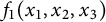 $f_1(x_1,x_2,x_3)$
,
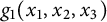 $g_1(x_1,x_2,x_3)$
, and
 $h_1(x_1,x_2,x_3)$
are given by (15), and let
 $R_1$
,
 $R_2$
, and
 $R_3$
be arbitrary functions that preserve the
 $T_1$
-reversible symmetry. Then, we have the following results:
-
i) (Fixed period) Let
$z_0$
be fixed such that
$ a_{400}(a_{200} + a_{201} z_0) < 0$
, and let
$\varepsilon $
be sufficiently small. Then, there exists a unique two-parameter family of initial conditions of the form
$(r(\varepsilon ), \theta (\varepsilon ), z(\varepsilon )) = (r_0 + \delta r(\varepsilon , \delta z), \frac {\pi }{2}, z_0)$
, with
$\delta r(0,0) = 0$
, such that each initial condition gives rise to a
$T_1$
-reversible symmetric periodic solution of the system (4) with fixed period
$T = 2\pi $
. Moreover, these solutions are close to the circular solution of radius
$r_0 = \frac {\sqrt {5}}{2} \sqrt {\frac {-a_{200} - a_{201} z_0}{a_{400}}}$
and lie near the plane
$z = z_0$
. -
ii) (Fixed period) Let
$a_{201} \neq 0$
, and let
$\varepsilon $
be sufficiently small. Then, there exists a two-parameter family of initial conditions of the form
$(r(\varepsilon ), \theta (\varepsilon ), z(\varepsilon )) = (r_0, \frac {\pi }{2}, z_0 + \delta z(\varepsilon , \delta r))$
, with
$\delta z(0,0) = 0$
, such that each initial condition yields a
$T_1$
-reversible symmetric periodic solution of the system (4) with fixed period
$T = 2\pi $
. Moreover, these solutions are close to the circular solution of radius
$r_0$
and near the plane
$z_0 = -\frac {5 a_{200} + 4 a_{400} r_0^2}{5 a_{201}}$
.












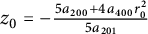
Now, we present an other example for the case of the reversible symmetry
 $T_2$
.
Example 2.2 Consider the system (2) with the following functions:
 $$ \begin{align} \begin{aligned} f_1(x_1,x_2,x_3)&= a_{210} x_1^2 x_2 + a_{030} x_2^3+ a_{012} x_2 x_3^2, \\ g_1(x_1,x_2,x_3)&= b_{120} x_1 x_2^2 + b_{101} x_1 x_3 + b_{002} x_3^2, \\ h_1(x_1,x_2,x_3)&= c_{110} x_1 x_2 + c_{011} x_2 x_3, \end{aligned} \end{align} $$
where
 $a_{ij}, b_{ij}$
, and
 $c_{ij}$
are arbitrary real numbers, and
 $R_1,R_2$
, and
 $R_3$
arbitrary functions that have the reversible symmetry
 $T_2$
. Clearly, this system is
 $T_2$
-reversible. Moreover, the previous functions (17) in cylindrical coordinates take the form:
 $$ \begin{align*} \tilde{f}_1(r,\theta, z) &= a_{210} r^3 \cos^2 \theta \sin \theta + a_{030} r^3 \sin^3 \theta+ a_{102} r z^2 \cos \theta, \\ \tilde{g}_1(r,\theta, z) &= b_{120} r^3 z \cos \theta \sin^2 \theta + b_{101} r z \cos \theta+ b_{002} z^2 , \\ \tilde{h}_1(r,\theta, z) &= c_{110} r^2 \cos \theta \sin \theta + c_{011} r z \sin \theta. \end{align*} $$
Next, we point out that the equation in item a) of Theorem 1.1 becomes
 $$ \begin{align} &\displaystyle \int_0^{\pi} \left[\tilde{g}_1(r_0,s, z_0) \cos s - \tilde{f}_1(r_0, s,z_0) \sin s \right] d s\nonumber\\&\qquad = \frac{1}{8} \pi r_0 \left[4 z_0 (b_{101}- a_{012} z_0)+ r_0^2 (-3 a_{030}- a_{210}+ b_{120})\right]=0. \end{align} $$
To apply item i) of Theorem 1.1, we need to solve (18) for
 $r_0$
, whose solution is
 $$ \begin{align*}r_0= 2 \sqrt{\frac{(b_{101}-a_{012} z_0) z_0}{3 a_{030}+ a_{210}- b_{120}}}, \end{align*} $$
whether
 $$ \begin{align*}\frac{(b_{101}-a_{012} z_0) z_0}{3 a_{030}+ a_{210}- b_{120}}>0. \end{align*} $$
Condition b) of Theorem 1.1 becomes
 $$ \begin{align*}z_0 (-b_{101}+ a_{012} z_0) \neq 0. \end{align*} $$
On the other hand, if we want to apply the second part of Theorem 1.1, we have to solve (18) with respect to
 $z_0$
, so we find two solutions
 $$ \begin{align*}z_{0\pm}= \frac{b_{101} \pm \sqrt{b_{101}^2+ a_{102}(-3 a_{030}- a_{210}+ b_{120}) r_0^2}}{2 a_{012}}, \end{align*} $$
whether
 $b_{101}^2+ a_{102}(-3 a_{030}- a_{210}+ b_{120}) r_0^2>0$
. Condition c) of Theorem 1.1 becomes
 $$ \begin{align*}\pm \frac{\pi r_0}{2} \sqrt{b_{101}^2+ a_{102} (-3 a_{030}- a_{210}+ b_{120}) r_0^2 } \neq 0. \end{align*} $$
In conclusion, by Theorem 1.1, we have the following result.
Theorem 2.2. Consider the spatial system (2), where the functions
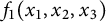 $f_1(x_1,x_2,x_3)$
,
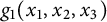 $g_1(x_1,x_2,x_3)$
, and
 $h_1(x_1,x_2,x_3)$
are as given in (17), and let
 $R_1$
,
 $R_2$
, and
 $R_3$
be arbitrary functions that preserve the
 $T_2$
-reversible symmetry. Then, we have the following results:
-
i) (Fixed period) Let
$z_0$
be fixed such that
$\frac {(b_{101} - a_{012} z_0) z_0}{3 a_{030} + a_{210} - b_{120}}> 0,$
and let
$\varepsilon $
be sufficiently small. Then, there exists a unique two-parameter family of initial conditions of the form
$(r(\varepsilon ), \theta (\varepsilon ), z(\varepsilon )) = \left (r_0 + \delta r(\varepsilon ), 0, z_0\right )$
, with
$\delta r(0,0) = 0$
, such that each initial condition gives rise to a
$T_2$
-reversible symmetric periodic solution of the system (4) with fixed period
$T = 2\pi $
. Moreover, these solutions are close to the circular solution of radius
$r_0 = 2 \sqrt {\frac {(b_{101} - a_{012} z_0) z_0}{3 a_{030} + a_{210} - b_{120}}},$
and lie near the plane
$z = z_0$
. -
ii) (Fixed period) Let
$r_0$
be fixed such that
$b_{101}^2 + a_{102}(-3 a_{030} - a_{210} + b_{120}) r_0^2> 0, a_{012} \neq 0,$
and let
$\varepsilon $
be sufficiently small. Then, there exist two families of initial conditions of the form
$(r(\varepsilon ), \theta (\varepsilon ), z(\varepsilon )) = \left (r_0, 0, z_{0\pm } + \delta z(\varepsilon )\right ),$
with
${\delta z(0,0) = 0}$
, such that each initial condition gives rise to a
$T_2$
-reversible symmetric periodic solution of the system (4) with fixed period
$T = 2\pi $
. Moreover, these solutions are close to the circular solution of radius
$r_0$
and near the plane
$z = z_{0\pm } = \frac {b_{101} \pm \sqrt {b_{101}^2 + a_{102}(-3 a_{030} - a_{210} + b_{120}) r_0^2}}{2 a_{012}}$
.














3 Proof of Theorem 1.2
Consider the system in
 $\mathbb {R}^3$
given by (2), and assume that it is
 $T_3$
-reversible symmetric, where
 $T_3(x_1, x_2, x_3) = (x_1, x_2, -x_3)$
. Note that
 $T_3$
represents a reflection with respect to the
 $x_1x_2$
-plane. The set of fixed points under
 $T_3$
is given by
 $$\begin{align*}\mathcal{L}_3 := \mathrm{Fix}(T_3) = \{(x_1, x_2, x_3) \in \mathbb{R}^3 : x_3 = 0\}, \end{align*}$$
which is a plane of dimension
 $\dim (\mathcal {L}_3) = 2$
. From the
 $T_3$
-reversibility condition, we obtain the following identities:
 $$ \begin{align*} f_1(x_1, x_2, -x_3) &= -f_1(x_1, x_2, x_3), g_1(x_1, x_2, -x_3)\\ & = -g_1(x_1, x_2, x_3), h_1(x_1, x_2, -x_3) = h_1(x_1, x_2, x_3). \end{align*} $$
Therefore, the functions
 $f_1$
and
 $g_1$
are odd in the variable
 $x_3$
, while
 $h_1$
is even in
 $x_3$
.
The characterization of the points in the set
 $\mathcal {L}_3$
in cylindrical coordinates is given by
 $z = 0$
. Moreover, the solution of the unperturbed system has the form
 $(r_0(t), \theta _0(t), z_0(t)) = (r_0, t + \theta _0, 0)$
, with initial condition
 $(r_0, \theta _0, 0) \in \mathcal {L}_3$
. Thus, it is a
 $2\pi $
-periodic circular solution of radius
 $r_0$
of the unperturbed system, lying in the plane
 $z = 0$
.
Lemma 3.1 A solution
 $(r(t, (r_0, \theta _0, z_0), \varepsilon ),\, \theta (t, (r_0, \theta _0, z_0), \varepsilon ),\, z(t, (r_0, \theta _0, z_0), \varepsilon ))$
of the perturbed system (4) is
 $2\pi $
-periodic and
 $T_3$
-reversible symmetric if we take
 $z_0 = 0$
and it satisfies the condition
 $z(\pi , (r_0, \theta _0, 0), \varepsilon ) = 0,$
where
 $(r_0, \theta _0, 0) \in \mathcal {L}_3$
is the initial condition.
Since
 $z_0 = 0$
, then by (9), the first-order approximation
 $z_1$
becomes
 $$ \begin{align} z_1(t, (r_0, \theta_0, 0)) = \int_0^t \tilde{h}_1(r_0, s + \theta_0, 0)\, ds, \end{align} $$
and the condition in Lemma 3.1 reduces to
 $$ \begin{align} z(\pi, (r_0, \theta_0, 0), \varepsilon) = \int_0^\pi \tilde{h}_1(r_0, s + \theta_0, 0)\, ds. \end{align} $$
To obtain families of
 $T_3$
-reversible symmetric periodic solutions with fixed period
 $T = 2\pi $
(or not fixed but close to
 $2\pi $
), we modify the initial condition by perturbing
 $r_0$
to
 $r_0 + \delta r$
, where
 $\delta r$
is a small parameter. That is, we consider a perturbation of the initial radius of the
 $T_3$
-symmetric circular solution of the unperturbed system. Then, equation (19) becomes
 $$ \begin{align} \mathcal{F}(\delta r, \varepsilon) = \int_0^{\pi} \tilde{h}_1(r_0 + \delta r, s + \theta_0, 0)\, ds + \mathcal{O}(\varepsilon), \end{align} $$
where, in this case,
 $\mathcal {F} : \mathbb {R} \times \mathbb {R} \rightarrow \mathbb {R}$
.
Now, by hypothesis
 $a),$
we have that
 $\mathcal {F}(0,0) = 0$
. In order to prove item
 $i)$
, we compute the following derivative:
 $$\begin{align*}\frac{\partial \mathcal{F}}{\partial \delta r} (\delta r, \varepsilon) = \int_0^{\pi} \frac{\partial\tilde{h}_1}{\partial r}(r_0 + \delta r, s + \theta_0, 0) \, ds. \end{align*}$$
Evaluating at
 $\delta r = 0$
and
 $\varepsilon = 0$
, by hypothesis
 $b),$
we get
 $$\begin{align*}\frac{\partial \mathcal{F}}{\partial \delta r} (0, 0) \neq 0, \end{align*}$$
thus, by the Implicit Function Theorem, the proof of item
 $i)$
follows.
For the case of variable period, we consider the function
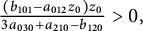
 $$ \begin{align} \overline{\mathcal{F}}(\tau, \delta r, \varepsilon) = \int_0^\tau \tilde{h}_1(r_0 + \delta r, s + \theta_0, 0)\, ds + \mathcal{O}(\varepsilon). \end{align} $$
By item
 $a)$
, we have
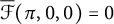 $\overline {\mathcal {F}}(\pi , 0, 0) = 0$
, and by item
 $c)$
,
 $$\begin{align*}\frac{\partial \overline{\mathcal{F}}}{\partial \tau}(\pi, 0, 0) = \tilde{h}_1(r_0, \pi + \theta_0, 0) \neq 0, \end{align*}$$
thus, again by the Implicit Function Theorem, the proof of item
 $ii)$
follows.
In order to compute the characteristic multipliers associated the family of the previous periodic solutions
 $\varphi (t, (r_0+\delta r,\theta _0,0),\varepsilon )=(r(t, (r_0+\delta r,\theta _0,0), \varepsilon ), \theta (t,(r_0+\delta r,\theta _0,0), \varepsilon ), z(t, (r_0+\delta r,\theta _0,0), \varepsilon ))$
, we consider the cross section
 $\Sigma =\{ \theta = 0\}$
for the system (5). Thus, to study the stability of the
 $T(\varepsilon )$
-periodic solutions
 $\varphi (t, (r_0+\delta r,0,0), \varepsilon )$
by considering the Poincaré map, we take
 $$ \begin{align} P_\varepsilon : \Sigma \rightarrow \Sigma, \quad (r, z) \mapsto P_\varepsilon(T(\varepsilon), r, z) = \left(r(T(\varepsilon), (r, 0, z), \varepsilon),\, z(T(\varepsilon), (r, 0, z), \varepsilon)\right), \end{align} $$
where
 $T(\varepsilon ) = 2\pi + \mathcal {O}(\varepsilon )$
.
We expand the flow components as:
 $$ \begin{align} r(T(\varepsilon), (r, 0, 0), \varepsilon) &= r + \varepsilon^{\alpha} r_1(T(\varepsilon), (r, 0, 0)) + \mathcal{O}(\varepsilon^{\alpha + 1}), \end{align} $$
 $$ \begin{align} z(T(\varepsilon), (r, 0, 0), \varepsilon) &= z + \varepsilon^{\alpha} z_1(T(\varepsilon), (r, 0, 0)) + \mathcal{O}(\varepsilon^{\alpha + 1}). \end{align} $$
Thus, the Poincaré map on
 $\Sigma $
becomes:
 $$ \begin{align} P_\varepsilon(r, z) = (r, z) + \varepsilon^{\alpha} \left(r_1(T(\varepsilon), (r, s, 0)), z_1(T(\varepsilon), (r, s, 0))\right) + \mathcal{O}(\varepsilon^{\alpha + 1}). \end{align} $$
In particular, the derivative of
 $P_\varepsilon $
with respect to
 $(r, z)$
takes the form:
 $$ \begin{align} D_{(r,z)} P_{\varepsilon}(r, z) = \mathcal{I} + \varepsilon^{\alpha} A + \mathcal{O}(\varepsilon^{\alpha + 1}), \end{align} $$
where
 $$\begin{align*}A_j &= \left(\begin{array}{@{}c}\displaystyle\int_0^{2 \pi}\left[\frac{\partial \tilde{f}_1}{\partial r} \cos \left(s+\theta_0\right)+ \frac{\partial \tilde{g}_1}{\partial r} \sin \left(s+\theta_0 \right)\right] ds \\ \displaystyle\int_0^{2 \pi} \frac{\partial \tilde{h}_1}{\partial r} ds \end{array}\right.\\&\quad\left.\begin{array}{cc}\displaystyle\displaystyle\int_0^{2 \pi}\left[\frac{\partial \tilde{f}_1}{\partial z} \cos \left(s+\theta_0\right)+ \frac{\partial \tilde{g}_1}{\partial z} \sin \left(s+\theta_0 \right)\right] ds \\ \displaystyle \displaystyle\int_0^{2 \pi} \frac{\partial \tilde{h}_1}{\partial z} ds\end{array}\right),\end{align*}$$
and each function in the integrands is evaluated at the initial condition
 $(r_0, s + \theta _0, 0)$
. According to our calculations, the parity of the functions
 $\tilde {f}_1$
,
 $\tilde {g}_1$
, and
 $\tilde {h}_1$
with respect to the variable s cannot be determined when evaluated at
 $\delta r = 0$
and
 $\varepsilon = 0$
under the symmetry
 $T_3$
. Therefore, the entries
 $a_{ij}$
of the matrix A are not necessarily zero. This enables the analysis of the characteristic multipliers, which correspond to the eigenvalues of A, providing information about the stability of the associated symmetric periodic solution. This concludes the proof of Theorem 1.2.
Now, we are going to show an example where we can apply Theorem 1.2.
Example 3.1 Consider the system (2) with the following functions:
 $$ \begin{align} \begin{aligned} f_1(x_1,x_2,x_3)&= a_{111} x_1 x_2 x_3+ a_{011} x_2 x_3+ a_{101} x_1 x_3, \\ g_1(x_1,x_2,x_3)&= b_{111} x_1 x_2 x_3 + b_{011} x_2 x_3 + b_{101} x_1 x_3, \\ h_1(x_1,x_2,x_3)&= c_{200} x_1^2 + c_{110} x_1 x_2 + c_{002} x_3^2 + c_{210} x_1^2 x_2 + c_{320} x_1^2 x_2^2 , \end{aligned} \end{align} $$
where
 $a_{ij}, b_{ij}$
, and
 $c_{ij}$
are arbitrary real numbers, and
 $R_1,R_2$
, and
 $R_3$
arbitrary but satisfying the reversible symmetry
 $T_3$
. Clearly, this system is
 $T_3$
-reversible. Moreover, the previous functions (28) in cylindrical coordinates take the form:
 $$ \begin{align*} \tilde{f}_1(r,\theta, z) &= a_{111} r^2 z \cos \theta \sin \theta + a_{011} r z \sin \theta +a_{101} r z \cos \theta, \\\tilde{g}_1(r,\theta, z) &= b_{111} r^2 z \cos \theta \sin \theta + b_{011} r z \sin \theta + b_{101} r z \cos \theta, \\\tilde{h}_1(r,\theta, z) &= c_{200} r^2 \cos ^2 \theta + c_{110} r^2 \sin \theta \cos \theta + c_{002} z^2 + c_{210} r^3 \sin \theta \cos ^2 \theta\\ &\quad + c_{320} r^4 \sin ^2 \theta \cos ^2 \theta. \end{align*} $$
We note that the equation in item a) of Theorem 1.1 reduces to
 $$ \begin{align} \int_0^\pi \tilde{h}_1(r_0, s+ \theta_0, 0) ds = \frac{r_0^2}{24} \left[3 \pi \left(4 c_{200}+c_{320} r^2 \right)+ 16 c_{210} r_0 \cos^3 \theta_0 \right]=0. \end{align} $$
To apply item i) of Theorem 1.2, we solve the equation for
 $r_0$
and for
 $c_{320} \neq 0$
, we obtain two possible roots, namely,
 $$ \begin{align} r_{0\pm} = \frac{ -8 c_{210} \cos ^3\theta_0 \pm 2 \sqrt{16 c_{210}^2 \cos ^6\theta_0-9 \pi ^2 c_{200} c_{320}}}{3 \pi c_{320}}. \end{align} $$
Now, we are going to analyze different situations according to the number of solutions.
Two distinct positive roots: This occurs when the discriminant is positive, i.e.,
 $$ \begin{align*}16 c_{210}^2 \cos^6 \theta_0 - 9 \pi^2 c_{200} c_{320}> 0, \end{align*} $$
and in addition, one of the conditions below is satisfied:
-
(i)
$ \theta _0 \in (\pi /2,3\pi /2) , \quad c_{320}> 0, \quad c_{210} > 0, \quad 0 < c_{200} < \dfrac {16 c_{210}^2 \cos ^6 \theta _0}{9 \pi ^2 c_{320}} $
, -
(ii)
$\theta _0 \in [0,\pi /2) \cup (3\pi /2,2\pi ], \quad c_{320}> 0, \quad c_{210} < 0, \quad 0 < c_{200} < \dfrac {16 c_{210}^2 \cos ^6 \theta _0}{9 \pi ^2 c_{320}} $
.


The previous set will be called
 $\Omega _1$
of parameters.
Unique positive root: We obtain one root when
 $c_{320} < 0,\ c_{200}> 0$
or
 $c_{320}> 0,\ c_{200} < 0$
. Or when occurs that,
 $$ \begin{align*}cos^6\theta_0 = \frac{9 \pi^2 c_{320} c_{200}}{16 c_{210}^2 }, \end{align*} $$
and one of the following conditions holds:
-
(i)
$ \theta _0 \in (\pi /2,3\pi /2) , \quad c_{210}> 0, \quad c_{320} < 0 $
, or
$ \quad c_{210} < 0, \quad c_{320}> 0$
. -
(ii)
$ \theta _0 \in [0,\pi /2) \cup (3\pi /2,2\pi ] , \quad c_{210}> 0, \quad c_{320} < 0 $
, or
$\quad c_{210} < 0, \quad c_{320}> 0 $
.




The previous set of parameters will be called
 $\Omega _2$
.
Now, the computation of the condition in item b) of Theorem 1.2 reduces to
 $$ \begin{align} \displaystyle\int_0^\pi \frac{\partial \tilde{h}_1}{\partial r} (r_0, s+\theta_0, 0) ds = \frac{A_{\pm}B_{\pm}}{27\pi^2 c_{320}^2}, \end{align} $$
where
 $$ \begin{align*} \begin{aligned} A_{\pm} &= -8 c_{210} \cos ^3\theta_0 \pm 2\sqrt{16 c_{210}^2 \cos ^6\theta_0-9 \pi ^2 c_{200} c_{320}} ,\\ B_{\pm} &= 9 \pi^2 c_{200} c_{320}-16 c_{210}^2 \cos ^6 \theta_0 \mp 4 c_{210} \cos ^3\theta_0 \sqrt{16 c_{210}^2 \cos ^6\theta_0-9 \pi ^2 c_{200} c_{320}}. \end{aligned} \end{align*} $$
It is verified that in the regions
 $\Omega _1$
and
 $\Omega _2$
that
 $A_{\pm }\neq 0$
and
 $B_{\pm } \neq 0$
. Therefore, conditions in items a) and b) are satisfied.
For the other case, the computation of the condition in item c) of Theorem 1.2 reduces to
 $$ \begin{align} \tilde{h}_1(r_0, \pi + \theta_0, 0) = r_0^2 \cos \theta_0 \left[ c_{110} \sin \theta_0 + \cos \theta_0 \left( c_{200}-c_{210} r_0 \sin \theta_0 + c_{320} r_0^2 \sin ^2\theta_0 \right)\right]. \end{align} $$
Now, if
 $r_0=r_{0\pm }$
as in (30), on the regions
 $\Omega _1$
and
 $\Omega _2$
, the condition
 $$ \begin{align*}\tilde{h}_1(r_{0\pm}, \pi + \theta_0, 0) = A_{+} B_1 \ or \ A_{-} B_2 \neq 0\end{align*} $$
is always satisfied if
 $B_i \neq 0$
, where
 $$ \begin{align*} \begin{aligned} A_{\pm} =\ & 4 \frac{\left(\sqrt{16 c_{210}^2 \cos^6\theta_0-9 \pi ^2 c_{200} c_{320}}\pm4 c_{210} \cos^3\theta_0 \right)^2 \cos \theta_0}{9 \pi ^2 c_{320}^2},\\B_1 =\; & c_{110} \sin \theta_0 + \frac{\cos \theta_0}{9 \pi^2 c_{320}} \Bigg( 4 \sin^2 \theta_0 \left( \sqrt{16 c_{210}^2 \cos^6 \theta_0 - 9 \pi^2 c_{200} c_{320}} + 4 c_{210} \cos^3 \theta_0 \right)^2 \\& + 6 \pi c_{210} \sin \theta_0 \cdot \left( \sqrt{16 c_{210}^2 \cos^6 \theta_0 - 9 \pi^2 c_{200} c_{320}} + 4 c_{210} \cos^3 \theta_0 \right) + 9 \pi^2 c_{200} c_{320} \Bigg),\\B_2 =\; & c_{110} \sin \theta_0 + \cos \theta_0 \Bigg( \frac{4 \sin^2 \theta_0 \big( \sqrt{16 c_{210}^2 \cos^6 \theta_0 - 9 \pi^2 c_{200} c_{320}} - 4 c_{210} \cos^3 \theta_0 \big)^2}{9 \pi^2 c_{320}} \\& \quad - \frac{2 c_{210} \sin \theta_0 \cdot \big( \sqrt{16 c_{210}^2 \cos^6 \theta_0 - 9 \pi^2 c_{200} c_{320}} - 4 c_{210} \cos^3 \theta_0 \big)}{3 \pi c_{320}} + c_{200} \Bigg). \end{aligned} \end{align*} $$
In conclusion, by Theorem 1.2, we obtain the following result.
Theorem 3.1. Consider the spatial system (2), where
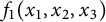 $f_1(x_1, x_2, x_3)$
,
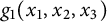 $g_1(x_1, x_2, x_3)$
, and
 $h_1(x_1, x_2, x_3)$
are as in (28), and let
 $R_1$
,
 $R_2$
, and
 $R_3$
be arbitrary functions possessing the symmetry
 $T_3$
. Then, we have the following:
-
i) (Fixed period) Let
$z = 0$
such that condition (31) is satisfied, and let
$\varepsilon $
be sufficiently small. If
$(c_{200}, c_{210}, c_{320}, \theta _0)$
satisfy the conditions of the set
$\Omega _1$
, then there exist two one-parameter families of initial conditions given by
$(r(\varepsilon ), \theta (\varepsilon ), z(\varepsilon )) = (r_{\pm } + \delta r_i(\varepsilon ), \theta _0, 0), \quad \delta r_i(0) = 0$
, such that they generate two
$T_3$
-reversible symmetric periodic solutions of system (4) with fixed period
$T = 2\pi $
. Moreover, these solutions are close to the circular ones with radius
$ r_{0\pm } = \frac {2 \left (-4 c_{210} \cos ^3 \theta _0 \mp \sqrt {16 c_{210}^2 \cos ^6 \theta _0 - 9 \pi ^2 c_{200} c_{320}} \right )}{3 c_{320} \pi },$
and lie close to the plane
$z = 0$
. -
ii) (Fixed period) Let
$z = 0$
such that condition (31) is satisfied, and let
$\varepsilon $
be sufficiently small. If
$(c_{200}, c_{210}, c_{320}, \theta _0)$
satisfy the conditions of the set
$\Omega _2$
, then there exists a one-parameter family of initial conditions
$(r(\varepsilon ), \theta (\varepsilon ), z(\varepsilon )) = (r_0 + \delta r(\varepsilon ), \theta _0, 0), \delta r(0) = 0$
, that generates a
$T_3$
-reversible symmetric periodic solution of system (4) with fixed period
$T = 2\pi $
. Moreover, this solution is close to the circular one with radius
$r_{0\pm } = \frac {2 \left (-4 c_{210} \cos ^3 \theta _0 \mp \sqrt {16 c_{210}^2 \cos ^6 \theta _0 - 9 \pi ^2 c_{200} c_{320}} \right )}{3 c_{320} \pi }$
, and close to the plane
$z = 0$
. -
iii) (Variable period) Let
$\varepsilon $
be sufficiently small and suppose
$(c_{200}, c_{210}, c_{320}, \theta _0)$
satisfy the conditions of the set
$\Omega _3 := \Omega _1 \cup \Omega _2$
. If
$B_i \neq 0$
, then there exists a differentiable function
$\tau (\delta r, \varepsilon )$
, such that
$\tau (0, 0) = \pi $
, and the full system (2) admits a two-parameter family of
$T_3$
-reversible symmetric periodic solutions parameterized by
$(\delta r, \varepsilon )$
, with period close to
$2 \tau (\delta r, \varepsilon ) = 2\pi + \mathcal {O}(\varepsilon ^\alpha )$
. Moreover, these solutions are close to a circular solution with radius
$r_{0\pm }$
and close to the plane
$z = 0$
.

























4 Proof of Theorem 1.3
Consider the system in
 $\mathbb {R}^3$
given by (2) and assume that the system admits the reversible symmetry
 $T_{j+4}$
for
 $j=1$
or
 $j=2$
. Consider the set of fixed points
 $\mathcal {L}_{j+4}=\{x_j=0,x_3=0\}$
with
 $dim (\mathcal {L}_{j+4})= 1$
. In cylindrical coordinates, the set
 $\mathcal {L}_{j+4}$
is characterized by
 $\theta \equiv \delta _j \frac {\pi }{2} \pmod \pi $
and
 $z = 0$
. Note that this set has two conditions, which is an important difference with respect to previous cases. Due to the reversible symmetry, the functions of the vector field satisfy the following properties: (a) for the symmetry
 $T_5$
, the functions
 $f_1$
and
 $h_1$
are even in the variables
 $(x_1, x_3)$
, while
 $g_1$
is odd in
 $(x_1, x_3)$
and (b) for the symmetry
 $T_6$
, the function
 $f_1$
is odd in the variables
 $(x_2, x_3)$
, and
 $g_1$
and
 $h_1$
are even in
 $(x_2, x_3)$
. In cylindrical coordinates, we have the following characterization.
Lemma 4.1 One solution
 $(r(t, (r_0,\theta _0,z_0),\varepsilon ),\theta (t, (r_0,\theta _0,z_0), \varepsilon ), z(t, (r_0,\theta _0,z_0),\varepsilon ))$
of the perturbed system (4) is
 $2 \pi $
-periodic and
 $T_{j+4}$
-reversible symmetric if it is satisfied the system
 $$ \begin{align} \begin{aligned} \theta\left(\pi, \left(r_0, \delta_j \frac{\pi}{2}, 0\right), \varepsilon \right) & =\delta_j \frac{\pi}{2} \ (\textit{mod}\ \pi), \\ z\left(\pi, \left(r_0, \delta_j \frac{\pi}{2}, 0\right), \varepsilon \right) & = 0, \end{aligned} \end{align} $$
where
 $(r_0, \delta _j \frac {\pi }{2}, 0) \in \mathcal {L}_{j+4}$
is the initial condition for
 $j=1$
and
 $j=2$
, respectively.
Next, the system of equations in (33) takes the form:
 $$ \begin{align} \begin{aligned}\theta\left(\pi,\left(r_0, \delta_j \frac{\pi}{2}, 0\right),\varepsilon\right)= &\ \pi + \delta_j \frac{\pi}{2}+ \frac{\varepsilon^{\alpha}}{r_0}\int_0^{\pi} \left[\tilde{g}_1\left(r_0, s+\delta_j \frac{\pi}{2},0\right) \cos \left(s+\delta_j \frac{\pi}{2}\right) \right. \\[0.5 pc] & \left. - \tilde{f}_1\!\left(\!r_0, s+\delta_j \frac{\pi}{2},0\!\right) \!\sin \!\left(\!s+\delta_j \frac{\pi}{2}\!\right)\!\right]\! ds + \!\mathcal{O}\left(\varepsilon^{\alpha+1}\right) = \delta_j \frac{\pi}{2} \ (\textit{mod}\ \pi), \\ z\left(\pi,\left(r_0,\delta_j \frac{\pi}{2}, 0\right),\varepsilon\right) = &\ \varepsilon^{\alpha} \int_0^{\pi} \tilde{h}_1\left(r_0,s+\delta_j \frac{\pi}{2},0\right) ds + \mathcal{O}(\varepsilon^{\alpha+1})=0, \end{aligned} \end{align} $$
and here we will consider the symmetry condition as
 $\theta (\pi ,(r_0,\delta _j \frac {\pi }{2}, 0),\varepsilon )= \pi + \delta _j \frac {\pi }{2}$
and
 $z(\pi ,(r_0,\delta _j \frac {\pi }{2}, 0),\varepsilon )=0$
. In order to obtain
 $T_{j+4}$
-reversible symmetric periodic solutions with period close to
 $T=2\pi $
, we modify the initial condition
 $(r_0, \delta _j \frac {\pi }{2}, 0)$
by taking
 $(r_0 + \delta r, \delta _j \frac {\pi }{2}, 0) \in \mathcal {L}_{j+4}$
for
 $j=1,2$
. Thus, the
 $T_{j+4}$
-reversible symmetric periodic solutions of the unperturbed system with initial condition
 $(r_0 + \delta r, \delta _j \frac {\pi }{2}, 0)$
are
 $(r_0(t), \theta _0(t), z_0(t)) = (r_0 + \delta r, \delta _j \frac {\pi }{2}, 0)$
. Moreover, for this symmetry, since there are two equations in (34) and two variables
 $(\delta r, \varepsilon )$
, it is necessary to include the time
 $\tau $
as an independent variable. Thus, the system (34) admits the following equivalent form:
 $$ \begin{align} \begin{array}{r@{\ }l} \mathcal{F}_1\left(\tau, \delta r,\varepsilon\right) & =\tau- \pi+ \frac{\varepsilon^{\alpha}}{r_0+ \delta r} \displaystyle \int_0^{\tau} \left[ \tilde{g}_1\left(r_0+\delta r, s+\delta_j \frac{\pi}{2}, 0\right) \cos \left(s+ \delta_j \frac{\pi}{2}\right) \right. \\[0.5 pc] &\quad -\left. \tilde{f}_1\left(r_0+\delta r, s+ \delta_j \frac{\pi}{2}, 0\right) \sin \left(s+\delta_j \frac{\pi}{2}\right)\right] ds + \mathcal{O}(\varepsilon^{\alpha+1}),\\ \mathcal{F}_2\left(\tau, \delta r,\varepsilon\right) & = \displaystyle \int_0^{\tau} \tilde{h}_1\left(r_0+\delta r, s+ \delta_j \frac{\pi}{2}, 0\right) ds + \mathcal{O}(\varepsilon). \end{array} \end{align} $$
Note that the function
 $\mathcal {F}=(\mathcal {F}_1, \mathcal {F}_2): \mathbb {R} \times \mathbb {R} \times \mathbb {R} \rightarrow \mathbb {R}^2$
. Thus, by hypotheses
 $a)$
and
 $b)$
, we get that
 $\mathcal {F}(\pi , 0,0)= (0, 0)$
. On the other hand,
 $$ \begin{align*}\frac{\partial (\mathcal{F}_1, \mathcal{F}_2)}{\partial (\tau, \delta r)} = \begin{pmatrix} 1 & \displaystyle\int_0^{\pi}\left[\frac{\partial \tilde{g}_1}{\partial r} \cos \left(s+\delta_j \frac{\pi}{2}\right) - \frac{\partial \tilde{f}_1}{\partial r} \sin \left(s+\delta_j \frac{\pi}{2}\!\right)\!\right] ds \\ \tilde{h}_1(r_0, \pi + \delta_j \frac{\pi}{2}, 0) & \displaystyle\int_0^{\pi} \frac{\partial \tilde{h}_1}{\partial r} ds \end{pmatrix}, \end{align*} $$
which is non-singular at
 $\tau = \pi , \delta r=0$
, and
 $\varepsilon =0$
, by hypothesis c) for
 $j=1$
or
 $j=2$
. Therefore, the proof of the theorem follows from the Implicit Function Theorem.
Example 4.1 Consider the system (2) with the following functions:
 $$ \begin{align} \begin{aligned} f_1(x_1,x_2,x_3)&= a_{222} x_1^2 x_2^2 x_3^2 + a_{202} x_1^2 x_3^2 + a_{022} x_2^2 x_3^2, \\ g_1(x_1,x_2,x_3)&= b_{110} x_1 x_2 + b_{011} x_2 x_3 + b_{300} x_1^3, \\ h_1(x_1,x_2,x_3)&= c_{220} x_1^2 x_2^2 + c_{202} x_1^2 x_3^2 + c_{022} x_2^2 x_3^2 + c_{240} x_1^2 x_2^4, \end{aligned} \end{align} $$
where
 $a_{ij}, b_{ij}$
, and
 $c_{ij}$
are arbitrary real numbers, and
 $R_1,R_2$
, and
 $R_3$
are arbitrary functions that have the reversible symmetry
 $T_5$
. Clearly, this system is
 $T_5$
-reversible. Moreover, the previous functions (36) in cylindrical coordinates take the form:
 $$ \begin{align*} \tilde{f}_1(r,\theta, z) &= a_{222} r^4 z^2 \cos^2 \theta \sin^2 \theta + a_{202} r^2 z^2 \cos^2 \theta + a_{022} r^2 z^2 \sin^2 \theta, \\ \tilde{g}_1(r,\theta, z) &= b_{110} r^2 \cos \theta \sin \theta + b_{011} r z \sin \theta + b_{300} r^3 \cos^3 \theta, \\ \tilde{h}_1(r,\theta, z) &= c_{220} r^4 \cos^2 \theta \sin^2 \theta + c_{202} r^2 z^2 \cos^2 \theta + c_{022} r^2 z^2 \sin^2 \theta + c_{240} r^6 \cos^2 \theta \sin^4 \theta. \end{align*} $$
Next, we point out that the integral in item a) of Theorem 1.3 becomes
 $$ \begin{align} \int_0^\pi \tilde{h}_1(r_0, s+ \pi/2, 0) ds = \frac{\pi r^4}{16} \left(2 c_{220}+c_{240} r^2\right). \end{align} $$
In order to apply item i) of Theorem 1.3, we need to solve the equation
 $$ \begin{align*}\frac{\pi r^4}{16} \left(2 c_{220}+c_{240} r^2\right)=0. \end{align*} $$
Then, there is a unique
 $r_0>0$
 $$ \begin{align*}r_0= \sqrt{2}\sqrt{-\frac{c_{220}}{c_{240}}}, \end{align*} $$
whether
 $c_{220} c_{240} <0$
. The calculation of condition b) of Theorem 1.3 becomes
 $$ \begin{align} \frac{ \displaystyle \pi c_{220}^{5/2}}{\sqrt{2} c_{240}^{3/2}}. \end{align} $$
In conclusion, by Theorem 1.3, we have the following result.
Theorem 4.1 Let the spatial system (2) with
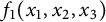 $f_1(x_1,x_2,x_3)$
,
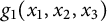 $g_1(x_1,x_2,x_3)$
, and
 $h_1(x_1,x_2,x_3)$
as in (36), and let
 $R_1, R_2$
, and
 $R_3$
be arbitrary functions possessing the symmetry
 $T_5$
. Assume that
 $c_{220} c_{240} < 0$
. Then, there exists a unique one-parameter family of initial conditions
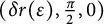 $(\delta r(\varepsilon ), \frac {\pi }{2}, 0)$
with
 $\delta r(0) = 0$
and a differentiable function
 $\tau (\varepsilon )$
such that each initial condition gives a
 $T_5$
-reversible symmetric periodic solution of the full system (2)
 $,$
with period
 $2 \tau (\varepsilon ) = 2 \pi + \mathcal {O}(\varepsilon ^{\alpha })$
. Moreover, these solutions are close to a circular solution with radius
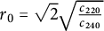 $r_0 = \sqrt {2} \sqrt {\frac {c_{220}}{c_{240}}}$
and lie on the
 $x_1 x_2$
-plane.
5 Concluding remarks
In this work, we have considered the following analytic (or
 $C^k-$
differentiable) family of ODE in
 ${\mathbb {R}}^3$
of the form:
 $$ \begin{align} \begin{array}{r@{\ }l} \dot{x_1} & = -x_2 + \varepsilon^{\alpha} f_1(x_1,x_2,x_3) + \varepsilon^{\alpha+1} R_1(x_1,x_2,x_3, \varepsilon), \\[0.5pc] \dot{x_2} & = x_1 + \varepsilon^{\alpha} g_1(x_1,x_2,x_3) + \varepsilon^{\alpha+1} R_2(x_1,x_2,x_3, \varepsilon),\\[0.5pc] \dot{x_3} & = \varepsilon^{\alpha} h_1(x_1,x_2,x_3)+ + \varepsilon^{\alpha+1} R_3(x_1,x_2,x_3, \varepsilon), \end{array} \end{align} $$
where
 $\alpha \in \mathbb {N}$
. Here,
 $\varepsilon $
is a small parameter. Note that the unperturbed system is
 $$ \begin{align*}\dot x_1= -x_2, \, \dot x_2= x_1, \, \dot x_3= 0, \end{align*} $$
which is foliated by circular solutions of fixed period
 $2 \pi $
on each plane
 $x_3 = x_{30}$
.
For our approach, we introduce cylindrical coordinates
 $ x_1 = \ r \cos \theta , \ x_2 = \ r \sin \theta , \ x_3 = \ x_3$
, then the system (39) takes the form:
 $$ \begin{align} \begin{aligned} \dot{r} & = \ \varepsilon^{\alpha}F_1(r,\theta,z) + \varepsilon^{\alpha+1}F_2(r,\theta,z) + \mathcal{O}(\varepsilon^{\alpha+2}) \\ \dot{\theta} & = 1+ \varepsilon^\alpha G_1(r,\theta,z) + \varepsilon^{\alpha+1}G_2(r,\theta,z)+\mathcal{O}(\varepsilon^{\alpha+2}) \\ \dot{z} & = \ \varepsilon^\alpha K_1(r,\theta,z) + \varepsilon^{\alpha+1}K_2(r,\theta,z) + \mathcal{O}(\varepsilon^{\alpha+2}), \end{aligned} \end{align} $$
where
 $$ \begin{align} \begin{aligned} F_1(r,\theta,z) & = \tilde{f}_1(r,\theta,z) \cos \theta + \tilde{g}_1(r,\theta,z)\sin \theta \\ G_1(r,\theta,z) & = \frac{1}{r} \left[\tilde{g}_1(r,\theta,z) \cos \theta - \tilde{f}_1(r,\theta,z) \sin \theta\right], \\ K_1(r,\theta,z)& = \tilde{h}_1(r,\theta,z), \end{aligned} \end{align} $$
with the functions
 $\tilde {f}_1(r, \theta , z)= f_1(r \cos \theta , r \sin \theta , z)$
,
 $\tilde {g}_1(r, \theta , z)= g_1(r \cos \theta , r \sin \theta , z),$
and
 $\tilde {h}_1(r, \theta , z)= h_1(r \cos \theta , r \sin \theta , z)$
.
In this work, we combine the reversible-discrete symmetries T of the system (39) and the Poincaré continuation method, strongly using the first approximation of the solutions of the full ordinary differential system given by a variational system. The main contribution of this article is to provide sufficient conditions for the existence of different families of reversible-symmetric periodic solutions for spatial perturbations (39) using cylindrical variables. Furthermore, we provide information about the characteristic multipliers of these solutions. We prove different theorems that give sufficient conditions for the existence of two types of families of initial conditions that produce reversible-symmetric periodic solutions for the system (39). The first type corresponds to reversible-symmetric periodic solutions with the same period as the circular orbit of the unperturbed system. The second type corresponds to reversible-symmetric periodic solutions with variable period, but close to that of the unperturbed circular orbit.
We point out that the periodicity equations (conditions for the existence of reversible-symmetric periodic solutions) depend on the dimension of the fixed point set S. Since S can be a reflection with respect to the plane
 $x=0$
, or
 $y=0$
, or
 $z=0$
, or a reflection with respect to the straight lines
 $x=y=0$
,
 $x=z=0$
, or
 $y=z=0$
, it follows that
 $S)$
can be 1 or 2. In the case
 $\dim (S)=2,$
there is only one condition to be satisfied, while in the case
 $\dim (S)=1,$
two conditions must be satisfied.
The importance of stating many theorems as results in this work lies in the different cases obtained by imposing a reversible symmetry on the system (39) in order to find symmetric periodic solutions, which is the main objective of this work. Hence, the relevance lies in the set of fixed points for each symmetry and their corresponding periodicity equations, as well as in the conditions required to apply the Implicit Function Theorem. We would like to highlight the impossibility of applying our method for certain symmetries. For the reversible symmetry
 $T_4(x_1, x_2, x_3)= (-x_1, -x_2, x_3)$
, we have
 $\mathcal {L}_4 = \mathrm {Fix}(T_4): x_1 = x_2 = 0$
. In cylindrical coordinates, a solution with
 $r> 0$
would be
 $T_4$
-reversible symmetric if
 $\theta _0 = 0$
and
 $\theta _0 = \pi /2 \ (\mathrm {mod}\ \pi )$
simultaneously, which is impossible.
5.1 A comparison with the averaging method
In order to complement our study, we analyze the possibility of using the Averaging method. We conclude that it is not possible to use this method in some cases due to the degeneracy of the averaging function at its zeros.
We start our analysis by considering the variable
 $\theta $
as a new time parameter, so the system (4) assumes the form:
 $$ \begin{align} \begin{aligned} \frac{d r}{d \theta} = & \ \frac{\varepsilon^{\alpha}F_1(r,\theta,z) + \varepsilon^{\alpha+1} F_2(r,\theta,z) + \mathcal{O}(\varepsilon^{\alpha+2})}{1+ \varepsilon^\alpha G_1(r,\theta,z) + \varepsilon^{\alpha+1} G_2(r,\theta,z)+ \mathcal{O}(\varepsilon^{\alpha+2})},\\ \frac{d z}{d \theta} = & \ \frac{\varepsilon^{\alpha}K_1(r,\theta,z) + \varepsilon^{\alpha+1} K_2(r,\theta,z) + \mathcal{O}(\varepsilon^{\alpha+2})}{1+ \varepsilon^\alpha G_1(r,\theta,z) + \varepsilon^{\alpha+1} G_2(r,\theta,z) + \mathcal{O}(\varepsilon^{\alpha+2})}. \end{aligned} \end{align} $$
Making the respective Taylor series approximation and
 $\varepsilon =0$
, we obtain the new equations
 $$ \begin{align} \begin{aligned} \frac{d r}{d \theta} & = \varepsilon^{\alpha} F_1(r,\theta,z) + \varepsilon^{\alpha+1} \left[F_2(r,\theta,z)-F_1(r,\theta,z)G_1(r,\theta,z)\right] + \mathcal{O}(\varepsilon^{\alpha +2} ),\\ \frac{d z}{d \theta} & = \varepsilon^{\alpha} K_1(r,\theta,z) +\varepsilon^{\alpha+1}\left[K_2(r,\theta,z)-K_1(r,\theta,z)G_1(r,\theta,z)\right] + \mathcal{O}(\varepsilon^{\alpha+2} ), \end{aligned} \end{align} $$
where
 $F_1,G_1$
, and
 $K_1$
are as (41) and
 $F_2= \tilde {f}_2(r,\theta ,z) \cos \theta + \tilde {g}_2(r,\theta ,z)\sin \theta $
and
 $K_2=\tilde {h}_2(r,\theta ,z),$
where
 $\tilde {f}_2(r,\theta ,z)=f_2(r \cos \theta , r \sin \theta ,z),\tilde {g}_2(r,\theta ,z)=g_2(r \cos \theta , r \sin \theta ,z),$
and
 $\tilde {h}_2(r,\theta ,z)=h_2(r \cos \theta , r \sin \theta ,z)$
. Moreover,
 $\tilde {f}_2,\tilde {h}_2$
are odd functions in
 $\theta $
and
 $\tilde {h}_2$
is even in
 $\theta $
. Now, we obtain the averaged functions for the first order,
 $$ \begin{align} \overline{F}_1(r,z) = \int_0^{2 \pi} F_1(r,z,\theta) d\theta,\quad \overline{K}_1(r,z) = \int_0^{2 \pi} K_1(r,z,\theta) d\theta. \end{align} $$
We call the attention that in order to apply the Averaging theorem of first order, we need initially to find
 $(r_0,z_0)$
such that,
 $$ \begin{align} \overline{F}_1(r_0,z_0) = 0, \quad \overline{K}_1(r_0,z_0)= 0, \end{align} $$
i.e., we need to solve a system of two equations. In particular, in order to find
 $(r_0,z_0)$
for this, the method notes that we need to solve a system of two equations, this is an important difference with our approach in this work, because in some cases of our symmetries, we need to solve only one equation.
It is important to emphasize that the existence of a family of periodic solutions bifurcates from the point
 $(r_0,z_0)$
. We need to verify the additional condition of non-degeneration
 $$ \begin{align*} \det \begin{pmatrix} \displaystyle \frac{\partial \overline{K}_1}{\partial r} & \displaystyle \frac{\partial \overline{K}_1}{\partial \theta} \\[8pt] \displaystyle \frac{\partial \overline{F}_1}{\partial r} & \displaystyle \frac{\partial \overline{F}_1}{\partial \theta} \end{pmatrix}_{\big| \substack{r=r_0 \\ z=z_0}} \neq 0. \end{align*} $$
5.1.1 Analysis of the symmetry
$T_1$

We will analyze the integrals that define the functions
 $F_1$
and/or
 $K_1$
, assuming that the vector field associated with system (39) possesses the reversible symmetry
 $T_1$
.
Lemma 5.1 Assume that the vector field (2) has the
 $T_1$
symmetry. Then, we have the following:
-
(1)
$ \overline {F}_1(r,z) \equiv 0$
; -
(2)
$ \overline {K}_1(r,z) \equiv 0$
.


Proof Under the symmetry
 $T_1$
, we have the following symmetry properties with respect to the angular variable
 $\theta $
:
 $$ \begin{align} \begin{aligned} \tilde{f}_1(r,\theta,z)= \tilde{f}_1(r,\pi-\theta,z), \tilde{g}_1(r,\theta,z)= -\tilde{g}_1(r,\pi-\theta,z), \tilde{h}_1(r,\theta,z)= -\tilde{h}_1(r,\pi-\theta,z). \end{aligned} \end{align} $$
Then, it is verified that
 $F_1(r,\pi -\theta ,z)=-F_1(r,\theta ,z),\ G_1(r,\pi -\theta ,z)=G_1(r,\theta ,z),$
and
 $K_1(r,\pi -\theta ,z)=-K_1(r,\theta ,z)$
. Let
 $u=\pi -\theta $
be a coordinate change, then
 $$ \begin{align*} \displaystyle \int_0^{ \pi} F_1(r,\theta,z) d\theta &= \displaystyle - \int_{\pi}^{ 0} F_1(r,\pi-u,z) du = \int_0^{ \pi} F_1(r,\pi-u,z) du\\& = -\int_0^{ \pi} F_1(r,u,z)du. \end{align*} $$
Returning to the variable
 $\theta ,$
we have that
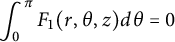 $\displaystyle \int _0^{ \pi } F_1(r,\theta ,z) d\theta = 0$
. Similarly, making the change of coordinates
 $u=3\pi -\theta $
, we can prove that
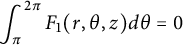 ${\displaystyle \int _\pi ^{ 2\pi } F_1(r,\theta ,z) d\theta = 0}$
. Analogously to the previous process, we prove that
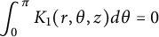 $\displaystyle \int _0^{ \pi } K_1(r,\theta ,z) d\theta = 0$
and
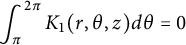 $\displaystyle \int _\pi ^{ 2\pi } K_1(r,\theta ,z) d\theta = 0$
.
Remark 3. From the previous lemma, it is clear that the first-order Averaging theory cannot be applied if the vector field in (2) or (39) possesses the reversible symmetry
 $T_1$
. In particular, the first-order Averaging method fails to yield periodic solutions in our Example 2.1, where
 $f_1$
,
 $g_1$
, and
 $h_1$
are as given in (15).
Motivated by the results in [Reference Llibre, Novaes and Teixeira20], we must examine whether any conclusions about the existence of periodic solutions can be obtained via the second-order averaging theory. For this, it is necessary to calculate the solutions of the system
 $\tilde {F}_2=0$
and
 ${\tilde {K}_2=0,}$
where
 $$ \begin{align} \begin{aligned} \tilde{F}_2(r,z) & = \int_0^{2\pi} \left[F_2(r,\theta,z)-F_1(r,\theta,z)G_1(r,\theta,z)\right]d\theta,\\ \tilde{K}_2(r,z) & = \int_0^{2\pi} \left[K_2(r,\theta,z)-K_1(r,\theta,z)G_1(r,\theta,z)\right]d\theta. \end{aligned} \end{align} $$
By the symmetry
 $T_1$
, we have the following symmetry properties with respect to the angular variable
 $\theta $
:
 $$ \begin{align} \begin{aligned} \tilde{f}_2(r,\theta,z)= & \tilde{f}_2(r,\pi-\theta,z), \\ \tilde{g}_2(r,\theta,z)= & -\tilde{g}_2(r,\pi-\theta,z), \\ \tilde{h}_2(r,\theta,z)= & -\tilde{h}_2(r,\pi-\theta,z). \end{aligned} \end{align} $$
Then, it verifies the following symmetry properties:
 $$ \begin{align} \begin{aligned} F_2(r,\pi-\theta,z)&=-F_2(r,\theta,z),\\ G_2(r,\pi-\theta,z)&=G_2(r,\theta,z),\\ K_2(r,\pi-\theta,z)&=-K_2(r,\theta,z). \end{aligned} \end{align} $$
We present the following result.
Lemma 5.2 Assume that the vector field (2) or (39) has the
 $T_1$
symmetry. Then, we have the following:
-
(1)
$\displaystyle \tilde {F}_2(r,z)=0$
; -
(2)
$\displaystyle \tilde {K}_2(r,z)=0$
.


Proof For item
 $(1)$
, we write
 $$ \begin{align*} \int_0^{ 2\pi} \left[F_2(r,\theta,z)-F_1(r,\theta,z)G_1(r,\theta,z)\right] d\theta& =\int_0^{ 2\pi}F_2(r,\theta,z)d\theta \\&\quad- \int_0^{ 2\pi}F_1(r,\theta,z)G_1(r,\theta,z)d\theta. \end{align*} $$
Since
 $F_2(r,\theta ,z) = -F_2(r,\pi -\theta ,z)$
, the integral
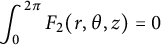 $\displaystyle \int _0^{2\pi }F_2(r,\theta ,z) = 0 $
, the proof is similar to item
 $(1)$
of Lemma 5.1. Now, we will focus on demonstrating
 $$ \begin{align*} \int_{0}^{2\pi} F_1(r,\theta,z)G_1(r,\theta,z)d\theta=0. \end{align*} $$
For this, rewrite the integral as
 $$ \begin{align*} \int_{0}^{2\pi} F_1(r,\theta,z)G_1(r,\theta,z)d\theta &= \int_{0}^{\pi} F_1(r,\theta,z)G_1(r,\theta,z)d\theta\\ &\quad +\int_{\pi}^{2\pi} F_1(r,\theta,z)G_1(r,\theta,z)d\theta. \end{align*} $$
If we take the change of coordinates
 $u=\pi -\theta $
and by the symmetry properties (49), we have that
 $$ \begin{align} \begin{aligned} \int_{0}^{\pi} F_1(r,\theta,z)G_1(r,\theta,z)d\theta & = -\int_{\pi}^{0} F_1(r,\pi-u,z)G_1(r,\pi-u,z)du, \\ & = -\int_{0}^{\pi} F_1(r,u,z)G_1(r,u,z)du. \end{aligned} \end{align} $$
So, we obtain that
 $\displaystyle \int _{0}^{\pi } F_1(r,\theta ,z)G_1(r,\theta ,z)d\theta =0$
. On the other hand, if we take the change of coordinates
 $u=3\pi -\theta $
, we get similarly that
 $\displaystyle \int _{\pi }^{2\pi } F_1(r,\theta ,z) G_1(r,\theta ,z)d\theta =0$
. Analogously, by performing the same procedure, we prove the result for item
 $(2)$
.
Remark 4 Consequently, the second-order averaging method yields no information regarding the existence of periodic solutions. Recursively, following the results in [Reference Llibre, Novaes and Teixeira20], the higher-order averaging theory also fails to provide information on the existence of periodic solutions.
5.1.2 Analysis of the symmetry
$T_2$

Now, we proceed to analyze the symmetry
 $T_2$
. In this case, we have the following result.
Lemma 5.3 Assume that the vector field (39) has the
 $T_2$
symmetry. Then, we have the following:
-
(1)
$ \overline {F}_1(r,z)=0$
; -
(2)
$ \overline {K}_1(r,z)=0$
.


Proof We know that
 $ F_1(r,\theta,z) = \tilde{f}_1(r,\theta,z) \cos \theta + \tilde{g}_1(r,\theta,z) \sin \theta$
and
 $ K_1(r,\theta,z) = \tilde{h}_1(r,\theta,z)$
. By the reversible symmetry T
2, the functions f
1 and h
1 are odd in the variable y, while g
1 is even. Consequently,
 $\tilde{f}_1$
and
 $\tilde{h}_1$
are odd functions of θ, and
 $\tilde{g}_1$
is even. It follows that both F
1 and K
1 are odd in θ, and therefore their integrals over a symmetric interval vanish.
Remark 5 Analogously to the previous case, we cannot apply the Averaging theory of first order if the vector field (2) or (39) possesses the reversible symmetry
 $T_2$
. In particular, we cannot obtain periodic solutions by the Averaging method of first order in our Example 2.2 with
 $f_1,g_1$
, and
 $h_1$
as in (17).
5.1.3 Analysis of the symmetry
$T_3$

To compare our results with our method and the theory of Averaging, we will concentrate on studying a polynomial vector field as in (39). The existence of the reversible implies that
 $f_1,g_1$
are odd in z and
 $h_1$
is even in z, this implies that
 $$ \begin{align*}f_1(x,y,z)=z \tilde{f}_1(x,y,z^2), \, g_1(x,y,z)=z \tilde{g}_1(x,y,z^2), \, \mathrm{and \ } h_1(x,y,z)= \tilde{h}_1(x,y,z^2), \end{align*} $$
for some polynomials
 $\tilde {f}_1, \tilde {g}_1$
, and
 $\tilde {h}_1$
. Then,
 $$ \begin{align*}\overline{F}_1(r,z)= z \displaystyle \int_0^{ 2\pi} \left[\tilde{f}_1(r,\theta,z^{2}) \cos \theta + \tilde{g}_1(r,\theta,z^{2})\sin \theta \right] d\theta. \end{align*} $$
Remark 6 From the previous calculus, we observe that
 $z_0=0$
can be part of an equilibrium point of the Averaging criteria of first order and
 $r_0$
must be computed by the equation
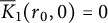 $\overline {K}_1(r_0,0)=0$
. On the other hand, in our main result for the reversible symmetry
 $T_3$
, that is, Theorem 1.2, we have that the continued periodic solutions bifurcate from the circular solution on the plane
 $z_0=0$
and
 $r_0$
is computed by the equation
 $\displaystyle \int _0^{\pi } \tilde {h}_1(r_0,\theta +\theta _0,0) ds=0$
. Therefore, we deduce that, in both methods,
 $z_0=0$
could generate periodic solutions.
Remark 7 We consider Example 3.1 in order to compare the applicability of the averaging method of the first order. We note that
 $$ \begin{align*}\overline{F}_1(r,z) & = \pi r z (a_{101}+b_{011}), \\ \overline{K}_1(r,z) & = \displaystyle \frac{1}{4} \pi \left(8 c_{002} z^2+4 c_{200} r^2+c_{320} r^4\right). \end{align*} $$
From this system, we obtain a unique equilibrium point
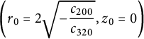 $\left (r_0=2 \sqrt { \displaystyle -\frac {c_{200}}{c_{320}}},z_0=0 \right )$
under the condition
 $c_{200}c_{320} <0 $
. It is verified that the determinant of its monodromy matrix is
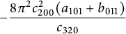 $ \displaystyle -\frac {8 \pi ^2 c_{200}^2 (a_{101}+b_{011})}{c_{320}}$
. If we impose that
 $(a_{101}+b_{011}) c_{200} \neq 0 $
, then by the Averaging theorem of first order, we obtain a unique family of periodic solution of period close to
 $2\pi $
which are close to the plane
 $z=0$
.
On the other hand, using our method
 $r_0$
must satisfy the equation
 $$ \begin{align*}\int_0^\pi \tilde{h}_1(r_0, s+ \theta_0, 0) ds = \frac{1}{24} r^2 \left[3 \pi \left(4 c_{200}+c_{320} r^2\right)+16 c_{210} r \cos^3 \theta_0 \right]=0. \end{align*} $$
From where given conditions on the parameters, we obtain
 $1$
or
 $2$
positive roots.
We point out that by Theorem 1.2, we obtain a family of initial conditions parameterized by
 $ \varepsilon $
, given by
 $ (r(\varepsilon ), \theta (\varepsilon ), z(\varepsilon )) = (r_0 + \delta r(\varepsilon ), \theta _0, 0) $
, where
 $ \theta _0 $
is initially arbitrary. The application of the Averaging method yields a different family of initial conditions of the form
 $ (\tilde {r}(\varepsilon ), \tilde {\theta }(\varepsilon ), \tilde {z}(\varepsilon )) = (r_0 + \mathcal {O}(\varepsilon ^3), 0, \mathcal {O}(\varepsilon ^3))$
. It is important to note that these two families of initial conditions are not the same. In Example 3.1 by the method presented in this work and the Averaging theory, the bifurcation of periodic solutions from the same point
 $(r_0,z_0=0)$
. Note that these families of initial conditions are not the same. In Figure 2, we show how these two different families of initial conditions are generated by both methods.
Families of initial conditions
 $(r(\varepsilon ),z(\varepsilon )=0)$
and
 $(r^*(\varepsilon ),z^*(\varepsilon ))$
parameterized by
 $\varepsilon $
, obtained by Theorem 1.2 and the Averaging theorem of first order, respectively, when the field (2) is under the reversible symmetry
 $T_3$
. Initially,
 $\theta =\theta _0$
is an arbitrary angle.
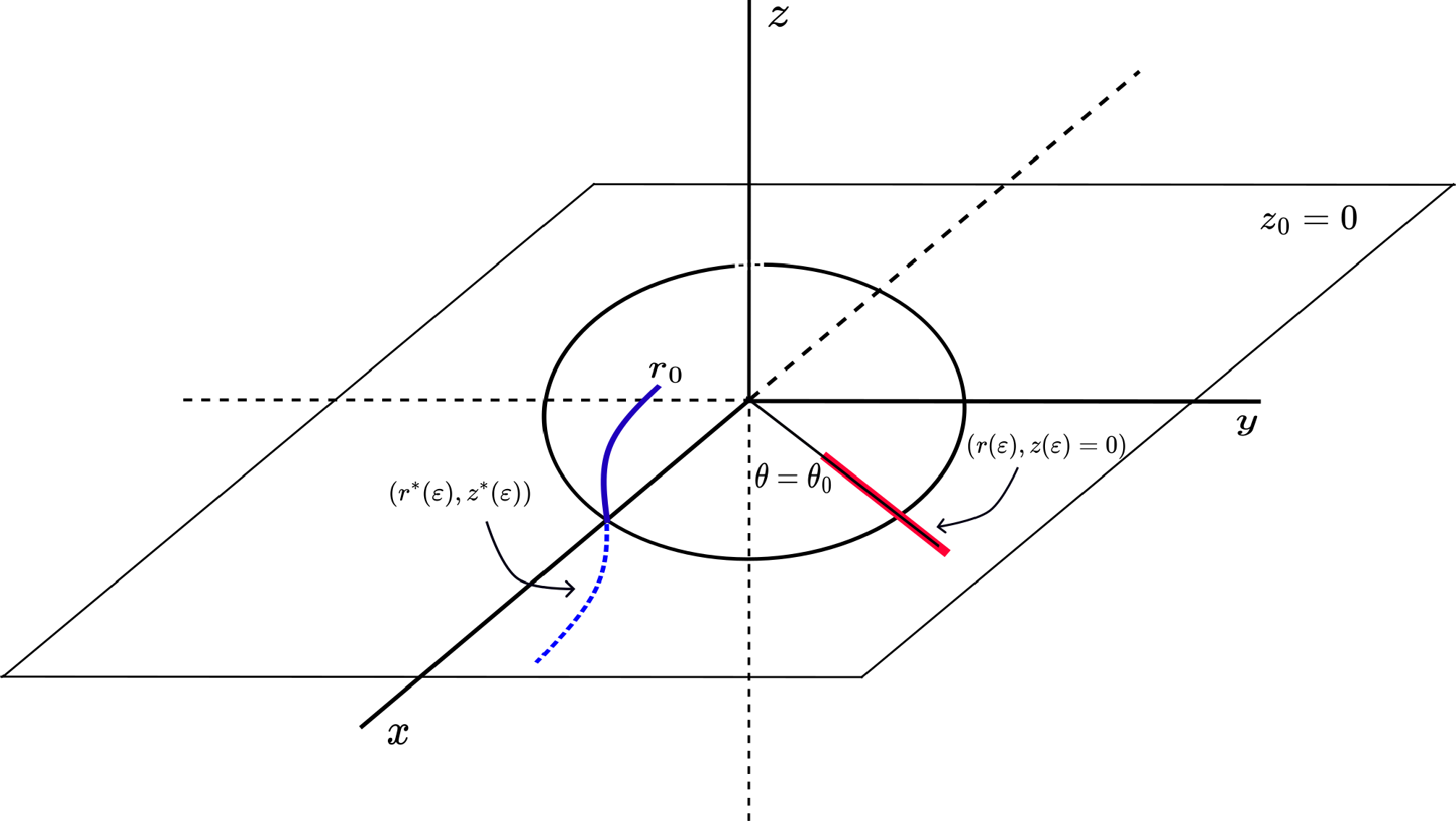
5.1.4 Analysis of the symmetry
$T_5$

For the purpose of analyzing the symmetry
 $T_5$
, we will assume that the functions
 $f_j,g_j,h_j$
are polynomials. So, we have that they can be written as
 $$ \begin{align*} f_1(x,y,z)& = f_{11}(x^2,y,z^2),\\ g_1(x,y,z)&= x\ g_{11}(x^2,y,z^2)+z\ g_{12}(x^2,y,z^2),\\ h_1(x,y,z)&= h_{11}(x^2,y,z^2). \end{align*} $$
For some polynomials
 $f_1,g_1$
, and
 $h_1$
. Now, we begin by presenting the following result.
Lemma 5.4 It verifies the following:
-
(1)
$\displaystyle \int _0^{2\pi } \cos ^{2\ell +1 }\theta \sin ^m \theta d\theta = 0$
, -
(2)
$\displaystyle \int _0^{2\pi } \cos ^{2\ell }\theta \sin ^m \theta d\theta = 0$
if m is odd, -
(3)
$\displaystyle \int _0^{2\pi } \cos ^{2\ell }\theta \sin ^m \theta d\theta = 2 \int _0^{\pi } \cos ^{2\ell }\theta \sin ^m \theta d\theta $
if m is even, -
(4)
$\displaystyle \int _0^{2\pi } \cos ^{2\ell + 1}\theta d\theta = 0$
, -
(5)
$\displaystyle \int _0^{2\pi } \cos ^{2\ell }\theta d\theta = 2\pi \frac {(2l)!}{2^{2l} (l!)^2}$
,

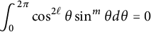

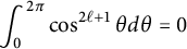
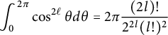
for
 $\ell ,m \in {\mathbb {N}}_0$
.
Lemma 5.5 Assume that the vector field (2) or (39) has the reversible symmetry
 $T_5$
. Then,
-
(1)
$\displaystyle \int _0^{ 2\pi } F_1(r,\theta ,z) d\theta = r z \int _{0}^{2\pi } \cos \theta \ \tilde {g}_{12}(r^2 \cos ^2 \theta ,r \sin \theta ,z^2) d\theta $
, -
(2)
$\displaystyle \int _0^{ 2\pi } K_1(r,\theta ,z) d\theta = 2 \int _0^{\pi } \tilde {h}_{11}(r^2 \cos ^2 \theta ,r \sin \theta ,z^2) d\theta $
.


Proof In cylindrical coordinates, the functions
 $f_1,g_1$
, and
 $h_1$
with the symmetry
 $T_5$
have the form:
 $$ \begin{align*} \begin{aligned} \tilde{f}_1(r,\theta,z) & =\tilde{f}_{11}(r^{2} \cos^{2}\theta,r \sin \theta,z^{2}), \\ \tilde{g}_1(r,\theta,z)& =r \cos \theta \ \tilde{g}_{11}(r^2 \cos^2 \theta,r \sin \theta,z^2)+z \ \tilde{g}_{12}(r^2 \cos^2 \theta,r \sin \theta,z^2), \\ \tilde{h}_1(r,\theta,z) & =\tilde{h}_{11}(r^{2} \cos^{2}\theta,r \sin \theta,z^{2}). \end{aligned} \end{align*} $$
Then, by equation (44), we have that
 $$ \begin{align*}F_1(r,\theta,z) & = \tilde{f}_{11}(r^{2} \cos^{2}\theta,r \sin \theta,z^{2}) \cos \theta\\&\quad + \left[ r \cos \theta \ \tilde{g}_{11}(r^2 \cos^2 \theta,r \sin \theta,z^2) + z \ \tilde{g}_{12}(r^2 \cos^2 \theta,r \sin \theta,z^2) \right]\sin \theta, \\ K_1(r,\theta,z)& = \tilde{h}_{11}(r^{2} \cos^{2}\theta,r \sin \theta,z^{2}). \end{align*} $$
Now, we analyze the following integrals that are part of the first equation in (44):
 $$ \begin{align*} I_1 &= \int_0^{2\pi} \tilde{f}_{11}(r^2 \cos^2 \theta,r \sin \theta, z^2) \cos \theta d\theta, \\ I_2 &= r\int_0^{2\pi} \cos \theta \sin \theta \ \tilde{g}_{11}(r^2 \cos^2 \theta,r \sin \theta, z^2)d\theta, \\ I_3 &= rz\int_0^{2\pi} \sin \theta \ \tilde{g}_{12}(r^2 \cos^2 \theta,r \sin \theta, z^2)d\theta. \end{align*} $$
It is verified that
 $I_1=0, I_2=0$
by virtue of the previous Lemma 5.4. Since the integrand is polynomial, it results in a combination of sine and cosine functions of that form:
 $$ \begin{align*}\cos^{2l+1}\theta \sin^m \theta, sin^{2l} \cos \theta, \end{align*} $$
and using the items of the previous Lemma 5.4, we obtain the result.
Remark 8 In general, it is not true that
 $\overline {F}_1 \equiv 0 $
and
 $ \overline {K}_1 \equiv 0 $
. In fact, we obtain
 $$ \begin{align*}\begin{array}{rl} \overline{F}_1(r,z) & = \pi b_{011} r z \\ \overline{K}_1(r,z) & = \displaystyle \frac{1}{8} \pi r^2 \left[ \left(8 z^2 (c_{022}+ c_{202})+2 c_{220} r^2+ c_{240} r^4 \right) \right]. \end{array} \end{align*} $$
Moreover, we obtain a unique zero given by
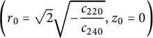 $\left (r_0=\sqrt {2} \sqrt { \displaystyle -\frac {c_{220}}{c_{240}}},z_0=0 \right )$
under the condition
 $c_{220}c_{240} <0 $
. It is verified that the determinant of its monodromy matrix is
 $ \displaystyle \frac {2 \pi ^2 b_{011} c_{220}^3}{c_{240}^2}$
. If we impose that
 $b_{011}c_{220}c_{240} \neq 0$
, we obtain a family of periodic solutions with period close to
 $2\pi $
by the Averaging method.
Now, as we see in Theorem 1.3 with
 $j=1$
, we obtain a family of initial conditions parameterized by
 $\varepsilon $
as follows
 $(r(\varepsilon ),\theta (\varepsilon ),z(\varepsilon ))=(r_0+\delta r(\varepsilon ), \pi /2,0)$
(with the same value of
 $r_0$
). However, by the use of the Averaging method, we obtain a family of initial conditions given by
 $(\tilde {r}(\varepsilon ),\tilde {\theta }(\varepsilon ),\tilde {z}(\varepsilon ))=(r_0 + \mathcal {O}(\varepsilon ^3),0 ,0 + \mathcal {O}(\varepsilon ^3))$
. Furthermore, we obtain, via our method and the Averaging theory, the bifurcation of periodic solutions from the same point
 $(r_0,z_0=0)$
. However, these families of initial conditions are not the same as shown in Figure 3.
Families of initial conditions
 $(r(\varepsilon ),z(\varepsilon )=0)$
and
 $(r^*(\varepsilon ),z^*(\varepsilon ))$
parameterized by
 $\varepsilon $
, obtained by Theorem 1.3 with
 $j=1$
(this is the
 $T_5$
-symmetry) and the Averaging theorem, respectively, when the field (2) is under the reversible symmetry
 $T_5$
and
 $\theta _0=\pi /2$
.
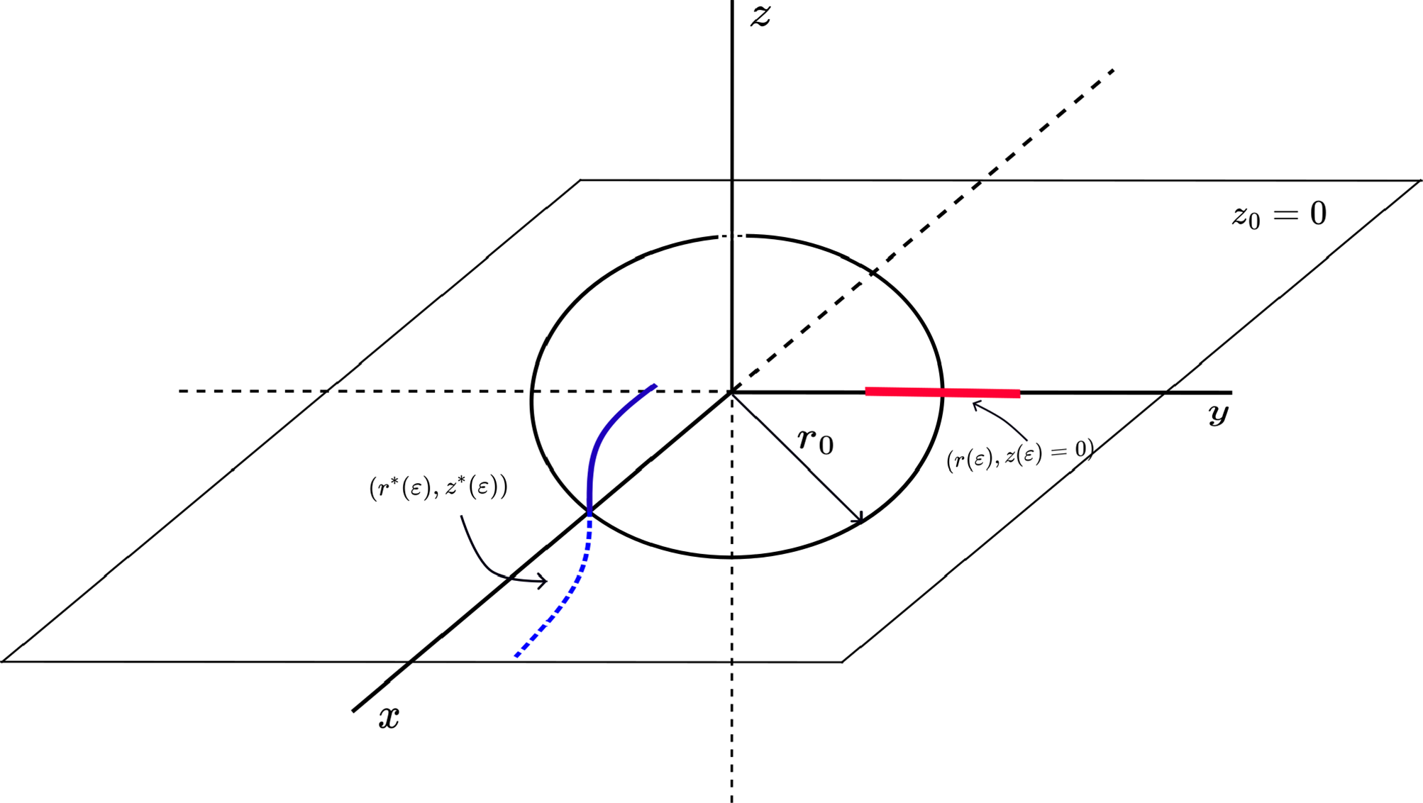
5.1.5 Analysis of the symmetry
$T_6$

For the purpose of analyzing the symmetry
 $T_6$
, we will again assume that the functions
 $f_1,g_1,h_1$
are polynomials. Then, by virtue of the symmetry, we have that
 $$ \begin{align*} f_1(x,y,z)& = y\ f_{11}(x,y^2,z^2)+z\ f_{12}(x,y^2,z^2),\\ g_1(x,y,z)&= g_{11}(x,y^2,z^2),\\ h_1(x,y,z)&= h_{11}(x,y^2,z^2) \end{align*} $$
for some polynomials
 $f_1,g_1$
, and
 $h_1$
. In cylindrical coordinates, the functions take the form:
 $$ \begin{align*} \tilde{f}_1(r,\theta,z)& = r \sin \theta \ \tilde{f}_{11}(r \cos \theta, r^2 \sin^2 \theta, z^2)+z\ \tilde{f}_{12}(r \cos \theta, r^2 \sin^2 \theta, z^2),\\ \tilde{g}_1(r,\theta,z)& = \tilde{g}_{11}(r \cos \theta, r^2 \sin^2 \theta, z^2),\\ \tilde{h}_1(r,\theta,z)& = \tilde{h}_{11}(r \cos \theta, r^2 \sin^2 \theta, z^2). \end{align*} $$
Lemma 5.6 Assume that the vector field (2) and (39) has the reversible symmetry
 $T_6$
. Then, we have the following:
 $\displaystyle \int _0^{ 2\pi } F_1(r,\theta ,z) d\theta = z \int _0^{2\pi } \tilde {f}_{12}(r \cos \theta , r^2 \sin ^2 \theta , z^2) \cos \theta d\theta $
,
 $\displaystyle \int _0^{ 2\pi } \tilde {h}_{11}(r \cos \theta ,r \sin ^2 \theta ,z^2) d\theta = 2 \int _0^{\pi } \tilde {h}_{11}(r \cos \theta ,r \sin ^2 \theta ,z^2) d\theta $
.
Proof By equation (44), the integral of
 $F_1$
takes the form:
 $$ \begin{align*} &\int_0^{2\pi} \left[ \big( r \sin \theta \ \tilde{f}_{11}(r \cos \theta, r^2 \sin^2 \theta, z^2)+z\ \tilde{f}_{12}(r \cos \theta, r^2 \sin^2 \theta, z^2) \big) \cos \theta\right. \\&\qquad \left.+ \tilde{g}_{11}(r \cos \theta, r^2 \sin^2 \theta, z^2) \sin \theta \right] d\theta \end{align*} $$
and we write it as the sum of the following three integrals:
 $$ \begin{align*} I_1 = & \int_0^{2\pi} r \sin \theta \tilde{f}_{11}(r \cos \theta,r^2 \sin^2 \theta, z^2) \cos \theta d\theta, \\ I_2 = & \int_0^{2\pi} z \ \tilde{f}_{12}(r \cos \theta,r^2 \sin^2 \theta, z^2) \cos \theta d\theta, \\ I_3 = & \int_0^{2\pi} \sin \theta \ \tilde{g}_1(r \cos \theta,r^2 \sin^2 \theta, z^2)d\theta. \end{align*} $$
It is verified that
 $I_1=0$
and
 $I_3=0$
due to the parity of the integrand, since they are odd in the variable
 $\theta $
. For the integral
 $I_2$
, we cannot say anything because the integrand is even in
 $\theta $
. Now, we rewrite the integral
 $$ \begin{align*} \displaystyle \int_0^{ 2\pi} \tilde{h}_1(r \cos \theta ,r \sin^2 \theta,z^2) &= \int_{0}^{\pi} \tilde{h}_1(r \cos \theta,r^2 \sin^2 \theta,z^2) d\theta\nonumber\\&\quad + \int_{\pi}^{2\pi} \tilde{h}_1(r \cos \theta,r^2 \sin^2 \theta,z^2) d\theta. \end{align*} $$
Let
 $u=2\pi -\theta $
be a change of coordinates and observe that
 $$ \begin{align*} \begin{aligned} \int_{\pi}^{2\pi} \tilde{h}_1(r \cos \theta,r^2 \sin^2 \theta,z^2) d\theta & = -\int_{\pi}^{0} \tilde{h}_1(r \cos (2\pi-u),r^2 \sin^2 (2\pi-u),z^2) du, \\ & = \int_{0}^{\pi} \tilde{h}_1(r \cos u, r^2 \sin^2 u,0) du. \end{aligned} \end{align*} $$
This concludes the proof.
Remark 9 By item
 $(1)$
of the previous Lemma 5.6, it is possible to apply the averaging method and obtain information about the existence of periodic solutions when the vector field (2) or (39) admits the reversible symmetry
 $T_6$
. Our objective now is to present the differences between both methods, highlighting the advantages and disadvantages of each. For this purpose, we will present three examples that we consider important to illustrate the relevance of these differences depending on the symmetry.
Example 5.1 Consider the system (2) with the following functions that admit symmetry
 $T_6$
:
 $$ \begin{align} \begin{aligned} f_1(x_1,x_2,x_3)&= a_{210} x_1^2 x_2 + a_{030} x_2^3+ a_{201} x_1^2 x_3, \\ g_1(x_1,x_2,x_3)&= b_{120} x_1 x_2^2 + b_{102} x_1 x_3^2 + b_{022} x_2^2 x_3^2, \\ h_1(x_1,x_2,x_3)&= c_{220} x_1^2 x_2^2 + c_{020} x_2^2+ c_{002} x_3^2 , \end{aligned} \end{align} $$
where
 $a_{ij}, b_{ij}$
, and
 $c_{ij}$
are arbitrary real numbers, and
 $R_1=R_2=R_3=0$
. The previous functions in cylindrical coordinates take the form:
 $$ \begin{align*} \tilde{f}_1(r,\theta, z) &= a_{210} r^3 \cos^2 \theta \sin \theta + a_{030} r^3 \sin^3 \theta + a_{201} z r^2 \cos^2 \theta, \\ \tilde{g}_1(r,\theta, z) &= b_{120} r^3 \cos \theta \sin^2 \theta + b_{102} r z^2 \cos \theta + b_{022} r^2 z^2 \sin^2 \theta, \\ \tilde{h}_1(r,\theta, z) &= c_{220} r^4 \cos^2 \theta \sin^2 \theta + c_{020} r^2 \sin^2 \theta + c_{002} z^2. \end{align*} $$
We verified that
 $\overline {F}_1(r,z)\equiv 0$
, thus, we cannot apply the Averaging method of first order.
Next, we present other important example for the analysis.
Example 5.2 Let
 $$ \begin{align} \begin{aligned} f_1(x_1,x_2,x_3)&= a_{210} x_1^2 x_2 + a_{030} x_2^3+ a_{201} x_1^2 x_3+a_{301} x^3 z, \\ g_1(x_1,x_2,x_3)&= b_{120} x_1 x_2^2 + b_{102} x_1 x_3^2 + b_{022} x_2^2 x_3^2, \\ h_1(x_1,x_2,x_3)&= c_{220} x_1^2 x_2^2 + c_{020} x_2^2+ c_{002} x_3^2 \end{aligned} \end{align} $$
be polynomials that admit the reversible symmetry
 $T_6$
, where
 $a_{ij}, b_{ij}$
, and
 $c_{ij}$
are arbitrary real numbers, and
 $R_1=R_2=R_3=0$
. The previous functions in cylindrical coordinates take the form:
 $$ \begin{align*} \tilde{f}_1(r,\theta, z) &= a_{210} r^3 \cos^2 \theta \sin \theta + a_{030} r^3 \sin^3 \theta + a_{201} z r^2 \cos^2 \theta + r^3 z \cos^3 \theta, \\ \tilde{g}_1(r,\theta, z) &= b_{120} r^3 \cos \theta \sin^2 \theta + b_{102} r z^2 \cos \theta + b_{022} r^2 z^2 \sin^2 \theta, \\ \tilde{h}_1(r,\theta, z) &= c_{220} r^4 \cos^2 \theta \sin^2 \theta + c_{020} r^2 \sin^2 \theta + c_{002} z^2. \end{align*} $$
We obtain that
 $$ \begin{align*} \overline{F}_1(r,z)& = \frac{3 a_{301} \pi}{4} r^3 z, \\ \overline{K}_1(r,z)& =\frac{1}{4} \pi \left( 8 c_{002} z^2+4 c_{020} r^2+ c_{220} r^4 \right). \end{align*} $$
This system has a zero with radius
 $r_0 = 2 \sqrt {\frac {c_{020}}{c_{220}}}$
and
 $z=0$
, when the condition
 $c_{202} c_{220}<0$
is satisfied.
Remark 10 By Theorem (1.3) with
 $j=2$
, the point
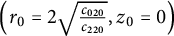 $\left (r_0 = 2 \sqrt { \frac {c_{020}}{c_{220}}},z_0=0\right )$
is exactly the point
 $(r_0,0)$
from which the
 $T_6$
-reversible symmetric periodic solution close to the
 $z=0$
-plane bifurcate. However, the curve of initial conditions that generated by the Averaging method is not the same curve of initial condition generated by our method, similar to happened with the symmetry
 $T_5$
, so in this case, the curve of initial condition is taken in
 $z_0=0$
and
 $\theta _0=0$
and it is on the x-axis as shown in Figure 4.
Families of initial conditions
 $(r(\varepsilon ),z(\varepsilon )=0)$
and
 $(r^*(\varepsilon ),z^*(\varepsilon ))$
parameterized by
 $\varepsilon $
, obtained by Theorem 1.3 with
 $j=2$
(this is, the
 $T_6$
-symmetry) and the Averaging theorem, respectively, when the field (2) has the reversible symmetry
 $T_6$
and
 $\theta _0=0$
.

Example 5.3 Consider the following polynomials:
 $$ \begin{align} \begin{aligned} f_1(x_1,x_2,x_3)= & a_{210} x_1^2 x_2 + a_{030} x_2^3+ z \left(a_{300} x^3+a_{500} x^5\right), \\ g_1(x_1,x_2,x_3)= & b_{120} x_1 x_2^2 + b_{102} x_1 x_3^2 + b_{022} x_2^2 x_3^2, \\ h_1(x_1,x_2,x_3)= & c_{220} x_1^2 x_2^2 + c_{020} x_2^2+ c_{002} x_3^2 , \end{aligned} \end{align} $$
that admit the
 $T_6$
-reversible symmetry,
 $a_{ij}, b_{ij}$
, and
 $c_{ij}$
are arbitrary real numbers, and
 $R_1=R_2=R_3=0$
. The previous functions in cylindrical coordinates take the form:
 $$ \begin{align*} \tilde{f}_1(r,\theta, z) &= a_{210} r^3 \cos^2 \theta \sin \theta + a_{030} r^3 \sin^3 \theta + z \left( a_{201} r^2 \cos^2 \theta + r^3 \cos^3 \theta\right), \\ \tilde{g}_1(r,\theta, z) &= b_{120} r^3 \cos \theta \sin^2 \theta + b_{102} r z^2 \cos \theta + b_{022} r^2 z^2 \sin^2 \theta, \\ \tilde{h}_1(r,\theta, z) &= c_{220} r^4 \cos^2 \theta \sin^2 \theta + c_{020} r^2 \sin^2 \theta + c_{002} z^2. \end{align*} $$
We have that
 $$ \begin{align*} \overline{F}_1(r,z)& = \frac{3 a_{301} \pi}{4} r^3 z, \\ \overline{K}_1(r,z)& =\frac{1}{4} \pi \left(8 c_{002} z^2+4 c_{020} r^2+c_{220} r^4\right). \end{align*} $$
Then, solving the equations
 $\overline {F}_1(r,z) = 0$
and
 $\overline {K}_1(r,z) =0$
, we obtain three no-degenerate isolated zeros
 $$ \begin{align*} r_0 &= 2 \sqrt{ \frac{c_{020}}{c_{220}} }, \quad z_0 = 0, \\ r_0 &= \sqrt{\frac{6}{5}} \sqrt{ \frac{a_{300}}{a_{500}} }, \quad z_0 = \frac{3}{10} \frac{ \sqrt{10\ a_{300}\ a_{500}\ c_{020} - 3 a_{300}^2\ c_{220}} }{ a_{500}\ \sqrt{c_{002}} }, \\ r_0 &= \sqrt{\frac{6}{5}} \sqrt{ \frac{a_{300}}{a_{500}} }, \quad z_0 = -\frac{3}{10} \frac{ \sqrt{10 a_{300}\ a_{500}\ c_{020} - 3 a_{300}^2\ c_{220}} }{ a_{500}\ \sqrt{c_{002}} }. \end{align*} $$
Thus, by the Averaging theorem of first order from each point, there are periodic solutions close to each plane
 $z_0$
, respectively. Now, using our Theorem 1.3, we obtain the existence of reversible symmetric periodic solutions close to circle with radius
 $r_0 = 2 \sqrt {\frac {c_{020}}{c_{220}}}$
on the plane
 $z_0=0$
under the condition that
 $c_{202} c_{220}>0$
.
Note that in this work, our analysis does not cover the case of double symmetry, because the vector field of system (2) does not form a group under the composition of its reversible symmetries, unlike what occurs in Hamiltonian systems (see, for example, [Reference Howison and Meyer14]).
In order to get an approximation of the reversible symmetric periodic solutions, we propose an approximation of the solution for the system (2):
 $$ \begin{align} \begin{aligned} x(t,\xi,\varepsilon) & = x_0(t)+\varepsilon^{\alpha} x_1(t)+ \mathcal{O}(\varepsilon^{\alpha+1}) \\ y(t,\xi,\varepsilon) & = y_0(t)+\varepsilon^{\alpha} y_1(t)+ \mathcal{O}(\varepsilon^{\alpha+1}) \\ z(t,\xi,\varepsilon) & = z_0(t)+\varepsilon^{\alpha} z_1(t)+ \mathcal{O}(\varepsilon^{\alpha+1}), \end{aligned} \end{align} $$
where
 $\xi =(x_0,y_0,z_0)$
is the initial condition. By the change of cylindrical variables, we have that
 $$ \begin{align} \begin{aligned} x(t) & = r(t) \cos \theta(t) \\ y(t) & = r(t) \sin \theta(t)\\ z(t) & = z(t), \end{aligned} \end{align} $$
where
 $(r(t),\theta (t),z(t))$
is as in (7). Thus, the approximation of the solution of the complete system is given by
 $$ \begin{align} \begin{aligned} x(t) & = (r_0(t)+\varepsilon^{\alpha}r_1(t)+\mathcal{O}(\varepsilon^{\alpha}))\cos (\theta_0(t)+\varepsilon^{\alpha}\theta_1(t)+\mathcal{O}(\varepsilon^{\alpha+1})),\\ y(t) & = (r_0(t)+\varepsilon^{\alpha}r_1(t)+\mathcal{O}(\varepsilon^{\alpha}))\sin (\theta_0(t)+\varepsilon^{\alpha}\theta_1(t)+\mathcal{O}(\varepsilon^{\alpha+1})), \\ z(t) & = z_0(t)+\varepsilon^{\alpha}z_1(t)+\mathcal{O}(\varepsilon^{\alpha+1}) \end{aligned} \end{align} $$
when
 $$ \begin{align} \begin{array}{l@{\ }l@{\ }l} x_0(t) & = r_0(t)\cos \theta_0(t),\\ y_0(t) & = r_0(t)\sin \theta_0(t),\\ z_0(t) & = z_0(t), \end{array} \begin{array}{l@{\ }l@{\ }l} x_1(t) & = r_1(t)\cos \theta_1(t),\\ y_1(t) & = r_1(t)\sin \theta_1(t),\\ z_1(t) & = z_1(t). \end{array} \end{align} $$
In our approach, it is possible to compute a second approximation of the solution but additional information is required.
Acknowledgements
This article is part of the Anderson Mercado Ph.D. thesis in the Program Doctorado en Matemática Aplicada, Universidad del Bío-Bío.