



1. Introduction
The Bessel process with constant drift was first studied in detail by Linetsky [Reference Linetsky23], who explicitly calculated the spectral representation of its transition density, making it statistically tractable. His motivation for studying this particular stochastic process stemmed from its applications in mathematical finance and queueing theory. In particular, [Reference Coffman, Puhalskii and Reiman8] presents the well-known heavy-traffic averaging principle (HTAP). In queueing theory language, this principle states that the work in each queue is emptied and refilled at a rate much faster than the rate at which the total workload changes. This implies that the total workload can be treated as approximately constant during the course of a cycle, while the individual queue workloads fluctuate in a fluid-like manner.
In polling systems (multi-queue systems where a single server visits queues in a fixed order), HTAP leads to a diffusion approximation involving the Bessel process with negative constant drift. Additionally, Linetsky shows that this process can be transformed into well-known models in mathematical finance, such as the
 $3/2$
model and the reciprocal of the square-root CIR process, thereby facilitating tractable pricing methods, for example, in the evaluation of Asian options [Reference Linetsky23].
Motivated by the analytical tractability and wide applicability of this process, we propose a new time-changed version of the Bessel process with constant drift. In our formulation, the time change is governed by the inverse of a stable subordinator, independent of the outer process. This extension introduces flexibility into the model and enables it to capture subdiffusive behavior and long-range dependence, phenomena frequently observed in complex systems. Such time-changed processes arise naturally when modeling power-law waiting times between particle jumps, and have proved useful across disciplines such as hydrology [Reference Chakraborty, Meerschaert and Lim6], biology [Reference Leonenko and Pirozzi18], and finance [Reference Fontana, Gnoatto and Szulda11]. For a broader perspective on the interplay between stochastic modeling, fractional calculus, and differential equations, see [Reference Meerschaert and Sikorskii25].
Since Linetsky’s foundational work, the Bessel process with constant drift has continued to attract significant interest, both theoretical and applied. Alternative closed-form expressions for its transition density have been derived in recent works [Reference Cui and Nguyen9, Reference Guarnieri, Moon and Wettlaufer13], though our analysis builds on Linetsky’s spectral approach. Moreover, the process has appeared as a special case of more general models driven by fractional Brownian motion [Reference Bishwal3]. Its applications span diverse domains: in climatology, it has been used to describe Arctic sea-ice thickness dynamics [Reference Toppaladoddi and Wettlaufer33, Reference Toppaladoddi and Wettlaufer34]; in biology, it models the dynamics of DNA bubble formation under thermal fluctuations [Reference Fogedby and Metzler10]; and in bird navigation, it appears under the name ‘pole-seeking Brownian motion’ [Reference Kendall15]. In conformal quantum mechanics, the process is linked to quantum Hamiltonians with Coulomb potentials [Reference Rajabpour29], which is also noted by Linetsky. Further applications in mathematical finance and economics can be found in [Reference Burtnyak and Malytska5] and [Reference Li21].
The structure of the paper is as follows. In Section 2 we briefly review key properties of the Bessel process with constant drift. Section 3 introduces the fractional Bessel process (with constant drift) and presents our main results. Specifically, we derive the spectral representation of its transition density and provide a strong solution to the corresponding fractional Cauchy problem. We also demonstrate that the stationary distribution remains the same as in the non-fractional case (a gamma distribution). Furthermore, the spectral representation enables us to compute the correlation structure of the (fractional) Bessel process, an expression not previously available in the literature, even for the non-fractional case. As a result, we establish that the process exhibits long-range dependence. Finally, in Section 4, we present concrete application of the model in queueing theory.
2. Bessel process
The Bessel process with constant drift was studied in detail in [Reference Linetsky23], where the spectral representation of the associated transition density was explicitly computed. The defining stochastic differential equation (SDE) for this process is
 \begin{equation}{\mathrm{d}} X(t)=\biggl(\dfrac{\nu+{\frac{1}{2}}}{X(t)}+\mu\biggr)\,{\mathrm{d}} t + {\mathrm{d}} B(t), \quad \nu \in (\! -1, +\infty ) \backslash \bigg\{\!-{\dfrac{1}{2}}\bigg\}, \ \mu \in \mathbb{R} \backslash \{0\},\end{equation}
where
 $(B(t), \, t \geq 0)$
denotes a standard Brownian motion. The state space of this process is
 $[ 0, +\infty)$
, and its parameters are
 $\mu$
and
 $\nu$
. The infinitesimal generator of the process is given by
 \begin{equation}\mathcal{G}f(x)=\biggl(\dfrac{\nu+{\frac{1}{2}}}{x}+\mu\biggr)\,f'(x)+\dfrac{1}{2}\,f''(x),\end{equation}
with the domain
 \begin{equation}D(\mathcal{G})=\biggl\{ f \in L^{2}([ 0, +\infty), \mathfrak{m}) \cap C^2( [ 0, +\infty) ) \colon \mathcal{G}f \in L^{2}([ 0, +\infty), \mathfrak{m} ), \ \lim_{x \downarrow 0}\dfrac{f'(x)}{\mathfrak{s}(x)}=0\biggr\},\end{equation}
where the speed and scale densities are
 \begin{equation*}\mathfrak{s}(x)=x^{-2\nu-1}\,{\mathrm{e}}^{-2\mu x}, \quad \mathfrak{m}(x)=2x^{2\nu +1}\,{\mathrm{e}}^{2\mu x}.\end{equation*}
If the parameter
 $\mu$
is positive, the process is transient, while for negative
 $\mu$
, the process admits a stationary distribution with gamma density
 \begin{equation}\pi(x)=\dfrac{-2\mu}{\Gamma(2\nu+2)}(\! -2\mu x)^{2\nu+1}\,{\mathrm{e}}^{2\mu x}, \quad x \geq 0.\end{equation}
We fully adopt the notation in [Reference Linetsky23], as our main result is an extension of that work.
The spectral representation of a stochastic process in this context involves solving the eigenvalue problem for the generator
 $\mathcal{G}$
(or equivalently, for the Sturm–Liouville operator
 $(\! -\mathcal{G})$
):
 \begin{equation*}(\! -\mathcal{G})f=\lambda \,f, \quad \lambda > 0.\end{equation*}
In general, the spectrum consists of two disjoint components: a discrete and a continuous (essential) part (see [Reference Linetsky22] and [Reference Reed and Simon30] for details).
In our setting, the discrete spectrum of
 $\mathcal{G}$
, given by (2.2), depends on the following parameter values.
-
• For
 $(\nu, \mu) \in (\! -{\tfrac{1}{2}}, +\infty ) \times (\! -\infty, 0 )$
: with eigenvalues
\begin{equation*}\sigma_d(\mathcal{G})=\biggl\{\dfrac{\mu^2}{2}\biggl(1-\biggl(\dfrac{\nu+{\frac{1}{2}}}{n+\nu+{\frac{1}{2}}}\biggr)^2\biggr), \,n \in \mathbb{N}_0\biggr\},\end{equation*}
(2.5)and eigenfunctions related to generalized Laguerre polynomials
\begin{equation}\lambda_n=\dfrac{\mu^2}{2}\biggl(1-\biggl(\dfrac{\nu+{\frac{1}{2}}}{n+\nu+{\frac{1}{2}}}\biggr)^2\biggr), \quad n \in \mathbb{N}_0,\end{equation}
$L_n^{2\nu}(x)$
, which solve The corresponding eigenfunctions are
\begin{equation*}xy''+ (2\nu+1-x )y'+ny=0, \quad n \in \mathbb{N}_0.\end{equation*}
(2.6)Note that the eigenvalues cluster near the constant
\begin{align} &\Psi_n(x)\nonumber\\ &\quad=\dfrac{n! \Gamma(1+2\nu)}{\Gamma(1+2\nu+n)}\exp\biggl({-\frac{n\mu x}{(\nu+n+{\tfrac{1}{2}})}}\biggr)\biggl(\! -2 \dfrac{\mu (\nu+{\tfrac{1}{2}})}{\nu+n+{\tfrac{1}{2}}}\biggr)^{\nu+1/2} L^{2\nu}_n \biggl(\! -2x \dfrac{\mu (\nu+{\tfrac{1}{2}})}{\nu+n+{\tfrac{1}{2}}}\biggr).\end{align}
$\mu^2/2$
.
-
• For
$(\nu, \mu) \in (\! -1, -{\tfrac{1}{2}} ) \times (\! -\infty, 0 )$
:
\begin{equation*}\sigma_d(\mathcal{G})=\{0\}.\end{equation*}
-
• For
$(\nu, \mu) \in (\! -{\tfrac{1}{2}}, +\infty ) \times ( 0, \infty )$
:
\begin{equation*}\sigma_d(\mathcal{G})=\emptyset.\end{equation*}
-
• For
$(\nu, \mu) \in (\! -1, -{\tfrac{1}{2}} ) \times ( 0, \infty )$
:
\begin{equation*}\sigma_d(\mathcal{G})=\biggl\{\dfrac{\mu^2}{2}\biggl(1-\biggl(\dfrac{\nu+{\frac{1}{2}}}{n+\nu+{\frac{1}{2}}}\biggr)^2\biggr), \,n \in \mathbb{N}_0\biggr\}.\end{equation*}









The essential part of the spectrum corresponds to the continuous spectrum
 \begin{equation}\sigma_c(\mathcal{G})=\biggl[\dfrac{\mu^2}{2}, +\infty\biggr),\end{equation}
while functions associated with the essential part of the spectrum are
 \begin{align}\Psi(x, \lambda)=x^{-\nu-1/2} \,{\mathrm{e}}^{-\mu x}M_{{\mathrm{i}} \beta/\sqrt{2\lambda-\mu^2}, \nu}\Bigl(\! -2{\mathrm{i}}\sqrt{2\lambda-\mu^2} x\Bigr), \end{align}
 \begin{align} \hat{\Psi}(x, \lambda)=x^{-\nu-1/2} \,{\mathrm{e}}^{-\mu x} W_{{\mathrm{i}} \beta/\sqrt{2\lambda-\mu^2}, \nu}\Bigl(\! -2{\mathrm{i}}\sqrt{2\lambda-\mu^2} x\Bigr),\end{align}
where
 \begin{align*}M_{\chi, \nu}(z)&\,:\!=\, z^{\nu+1/2}\,{\mathrm{e}}^{-z/2} M\biggl(\nu-\chi+\frac{1}{2};\,1+2\nu,z\biggr), \\W_{\chi, \nu}(z)&\,:\!=\, z^{\nu+1/2}\,{\mathrm{e}}^{-z/2} U\biggl(\nu-\chi+\frac{1}{2};\,1+2\nu,z\biggr), \quad -\pi < \arg(z)\leq \pi,\end{align*}
are the Whittaker functions, with
 $M(a,b;\,z)$
and
 $U(a,b;\,z)$
being first and second confluent hypergeometric functions (for details about Whittaker and related special functions, see e.g. [Reference Buchholz4]).
The Bessel process is a time-homogeneous diffusion. Let
 $p(x, t;\, y)$
denote its transition density:
 \begin{equation*}p(x, t;\, y) = \dfrac{{\mathrm{d}}}{{\mathrm{d}} x}\mathbb{P}(X(t) \leq x \mid X(0)=y).\end{equation*}
Define
 \begin{equation}\beta\,:\!=\, -\mu\biggl(\nu+\dfrac{1}{2}\biggr).\end{equation}
Notice that
 $\beta>0$
when
 $\mu <0$
and
 $\nu>-{\tfrac{1}{2}}$
, while
 $\beta<0$
in the case
 $\mu<0$
and
 $\nu\in(\! -1,-\frac{1}{2})$
. According to [Reference Linetsky23], the spectral representation of the transition density
 $p(x, t;\, y)$
of the Bessel process with constant drift (as defined by (2.1)) is given by
 \begin{equation}p(x,t;\,y)=p_d(x,t;\,y)+p_c(x,t;\,y),\end{equation}
where
 $p_d$
corresponds to the discrete spectrum contribution and
 $p_c$
to the continuous one. The explicit expressions for
 $ p_d $
and
 $ p_c $
vary depending on the values of
 $ \nu $
and
 $ \mu $
, and are given below. They reflect the decomposition of the transition density into discrete and continuous spectral components associated with the generator
 $ \mathcal{G}$
:
 \begin{align*}&p_d(x,t;\,y)\\&\ =\left\{\begin{array}{ll} \pi(x)+\sum\limits_{n=1}^{\infty}\dfrac{n!\beta(2\beta x)^{2\nu+1}}{\big(n+\nu+{\frac{1}{2}}\big)^{2\nu+3}\Gamma(2\nu+n+1)}L^{2\nu}_{n}\biggl(\dfrac{2 \beta x}{n+\nu+{\frac{1}{2}}}\biggr) & \\[13pt] \times\,\exp\biggl(2\mu x-\dfrac{\mu n}{n+\nu+\frac{1}{2}}(x+y)-\lambda_n t\biggr) L^{2\nu}_{n}\biggl(\dfrac{2 \beta y}{n+\nu+{\frac{1}{2}}}\biggr), & \big(\! -{\tfrac{1}{2}}, +\infty \big) \times (\! -\infty, 0 ),\\ \pi(x), & \big(\! -1, -{\tfrac{1}{2}} \big) \times (\! -\infty, 0 ),\\[2pt] 0, & \big(\! -{\tfrac{1}{2}}, +\infty \big) \times ( 0, +\infty ),\\ \sum\limits_{n=1}^{\infty}\dfrac{n!\beta(2\beta x)^{2\nu+1}}{\big(n+\nu+{\frac{1}{2}}\big)^{2\nu+3}\Gamma(2\nu+n+1)}L^{2\nu}_{n}\biggl(\dfrac{2 \beta x}{n+\nu+{\frac{1}{2}}}\biggr) & \\[14pt] \times\, \exp\biggl(2\mu x-\dfrac{\mu n}{n+\nu+\frac{1}{2}}(x+y)-\lambda_n t\biggr) L^{2\nu}_{n}\biggl(\dfrac{2 \beta y}{n+\nu+{\frac{1}{2}}}\biggr), & \big(\! -1, -{\tfrac{1}{2}} \big) \times ( 0, +\infty ),\end{array}\right.\end{align*}
where the sets on the right-hand side specify the corresponding range of
 $(\nu, \mu)$
, and
 \begin{align*}p_{c}(x,t;\,y)&=\dfrac{1}{2\pi}\int_{\mu^2/2}^{\infty}\dfrac{1}{k(\lambda)}\biggl|\dfrac{\Gamma({\frac{1}{2}}+\nu+{\mathrm{i}} \beta/ k(\lambda))}{\Gamma(1+2\nu)}\biggr |^2 \,{\mathrm{e}}^{-\lambda t}\biggl(\dfrac{x}{y}\biggr)^{\nu+{{1}/{2}}}\,{\mathrm{e}}^{\mu(x-y)+\pi \beta /k(\lambda)} \\&\quad \times M_{{\mathrm{i}} \beta/ k(\lambda),\, \nu}(\! -2{\mathrm{i}} k(\lambda) y) M_{-{\mathrm{i}} \beta/ k(\lambda), \, \nu}(2{\mathrm{i}} k(\lambda) x)\, {\mathrm{d}} \lambda ,\end{align*}
for
 $y>0$
, while
 \begin{align*}&p_d(x,t;\,0)\\&\ =\left\{\begin{array}{ll}\pi(x)+\sum\limits_{n=1}^{\infty}\dfrac{\beta(2\beta x)^{2\nu+1}}{\big(n+\nu+{\frac{1}{2}}\big)^{2\nu+3}\Gamma(2\nu+1)} & \\[15pt]\times\, \exp\biggl(2\mu x - \dfrac{\mu n}{n + \nu + \frac{1}{2}} x - \lambda_n t\biggr)L^{2\nu}_{n}\biggl(\dfrac{2 \beta x}{n+\nu+{\frac{1}{2}}}\biggr) , &\quad \big(\! -{\tfrac{1}{2}}, +\infty \big) \times (\! -\infty, 0 ),\\\pi(x) , & \quad \big(\! -1, -{\tfrac{1}{2}} \big) \times (\! -\infty, 0 ),\\[2pt]0 , & \quad \big(\! -{\tfrac{1}{2}}, +\infty \big) \times ( 0, +\infty ),\\\sum\limits_{n=1}^{\infty}\dfrac{\beta(2\beta x)^{2\nu+1}}{\big(n+\nu+{\frac{1}{2}}\big)^{2\nu+3}\Gamma(2\nu+1)} & \\[14pt]\times\, \exp\biggl(2\mu x - \dfrac{\mu n}{n + \nu + \frac{1}{2}} x - \lambda_n t\biggr) L^{2\nu}_{n}\biggl(\dfrac{2 \beta x}{n+\nu+{\frac{1}{2}}}\biggr) , &\quad \big(\! -1, -{\tfrac{1}{2}} \big) \times ( 0, +\infty ),\end{array}\right.\end{align*}
and
 \begin{align*}p_{c}&(x,t;\,0) \\ &=\dfrac{1}{2\pi}\int_{\mu^2/2}^{\infty}2^{\nu+1/2}k(\lambda)^{\nu - 1/2}\,{\mathrm{e}}^{{\mathrm{i}}\pi (\nu/2+1/4)}\biggl|\dfrac{\Gamma({\frac{1}{2}}+\nu+{\mathrm{i}} \beta/ k(\lambda))}{\Gamma(1+2\nu)}\biggr |^2 \,{\mathrm{e}}^{-\lambda t}x^{\nu+{{1}/{2}}}\,{\mathrm{e}}^{\mu x+\pi \beta /k(\lambda)} \\&\quad \times M_{{\mathrm{i}} \beta/ k(\lambda), \, \nu}(\! -2{\mathrm{i}} k(\lambda) x)\, {\mathrm{d}} \lambda,\end{align*}
for
 $y=0$
, where
 $k(\lambda)=\sqrt{2\lambda-\mu^2}$
(for details and the proof, see [Reference Linetsky23, Proposition 1]).
3. Fractional Bessel process
Let
 $ (D(t),\, t \geq 0) $
be a standard stable subordinator with index
 $ 0 < \alpha < 1 $
. This is a non-decreasing Lévy process characterized by the Laplace transform
 \begin{equation*}\mathbb{E}\big[{\mathrm{e}}^{-s D(t)}\big] = \exp(\! -t s^{\alpha}), \quad s \geq 0.\end{equation*}
We define the inverse subordinator (also known as the first passage or hitting time process) by
 \begin{equation}E(t) = \inf \{ x > 0 \colon D(x) > t \}, \quad t \geq 0.\end{equation}
The process
 $(E(t), \,t \geq 0)$
is non-Markovian and non-decreasing. For every fixed
 $ t \geq 0 $
, the random variable E(t) has a probability density function
 $ f_t(x) $
whose Laplace transform is given by
 \begin{equation} \mathbb{E}\big[{\mathrm{e}}^{-s E(t)}\big] = \int_{0}^{\infty} \,{\mathrm{e}}^{-s x} f_t(x)\, {\mathrm{d}} x = \mathcal{E}_{\alpha}(\! -s t^{\alpha}),\end{equation}
where
 \begin{equation*}\mathcal{E}_{\alpha}(z) \,:\!=\, \sum_{j=0}^{\infty} \dfrac{z^j}{\Gamma(1 + \alpha j)}, \quad z \in \mathbb{C},\end{equation*}
is the Mittag–Leffler function, which converges absolutely for all complex z (see e.g. [Reference Gorenflo, Kilbas, Mainardi and Rogosin12]).
The fractional Bessel process is defined as the time-changed Bessel process via the inverse of the stable subordinator:
 \begin{equation}X_{\alpha}(t)\,:\!=\, X(E(t)),\end{equation}
where
 $(X(t), \, t \geq 0)$
is the Bessel process corresponding to the SDE (2.1) and
 $(E(t), \, t \geq 0)$
is the inverse
 $\alpha$
-stable subordinator (3.1), assumed to be independent of the Bessel process. We emphasize that the resulting process is non-Markovian, but nevertheless the function
 $p_{\alpha}(x,t;\,y)$
such that
 \begin{equation*}\mathbb{P}(X_{\alpha}(t) \in B \mid X_{\alpha}(0)=y)=\int_{B}p_{\alpha}(x,t;\,y)\,{\mathrm{d}} x\quad \text{for any Borel subset }\textit{B}\, \text{of } [0,+\infty)\end{equation*}
will be referred to as transition density of the fractional Bessel process.
3.1. Spectral representation of transition density of the fractional Bessel process
In order to prove the main result, we first state and prove two technical lemmas.
Lemma 3.1. Let
 $\nu \in (\! -1, +\infty ) \setminus \{\!-\frac{1}{2}\}, \, \mu \in \mathbb{R} \setminus \{0\}$
and
 $\beta$
given by (2.10), with
 $\mathcal{E}_{\alpha}(\!\cdot\!)$
denoting Mittag–Leffler function and
 $L^{2\nu}_{n}(\!\cdot\!)$
the generalized Laguerre polynomial. Then, for
 $x \geq 0, y >0$
,
 \begin{align*}&\sum_{n=1}^{\infty}\dfrac{n!\beta(2\beta x)^{2\nu+1}\exp\bigl(2\mu x - \frac{\mu n}{n + \nu +1/2}(x+y)\bigr)}{\big(n+\nu+{\frac{1}{2}}\big)^{2\nu+3}\Gamma(2\nu+n+1)}\mathcal{E}_{\alpha}(\! -\lambda_n t^{\alpha})\biggl|L^{2\nu}_{n}\biggl(\dfrac{2 \beta x}{n+\nu+{\frac{1}{2}}}\biggr) L^{2\nu}_{n}\biggl(\dfrac{2 \beta y}{n+\nu+{\frac{1}{2}}}\biggr)\biggr| \\&\quad < \infty,\end{align*}
while for
 $x \geq 0$
,
 \begin{equation*}\sum_{n=1}^{\infty}\dfrac{\beta(2\beta x)^{2\nu+1}}{\big(n+\nu+{\frac{1}{2}}\big)^{2\nu+3}\Gamma(2\nu+1)}\exp\biggl(2\mu x - \frac{\mu n x}{n + \nu + \frac{1}{2}}\biggr)\mathcal{E}_{\alpha}(\! -\lambda_n t^{\alpha})\biggl|L^{2\nu}_{n}\biggl(\dfrac{2 \beta x}{n+\nu+{\frac{1}{2}}}\biggr) \biggr| < \infty.\end{equation*}
Proof. In order to prove the convergence of the series, it is sufficient to show that for large values of n, the terms are bounded by those of a convergent series.
According to [Reference Sansone31, p. 348, (36)], we have
 \begin{equation*}L^{2\nu}_{n}\biggl(\dfrac{2 \beta x}{n+\nu+{\frac{1}{2}}}\biggr) \thicksim {\mathrm{O}} \bigl((2\beta x)^{-1/4-\nu}n^{2\nu}\bigr), \quad n \to \infty.\end{equation*}
On the other hand, the sequence
 $(\lambda_n, \, n \in \mathbb{N} )$
, where
 $\lambda_n$
is given by (2.5), is an increasing sequence of eigenvalues such that
 \begin{equation*}\lim_{n \to \infty}\lambda_n=\dfrac{\mu^2}{2}.\end{equation*}
Therefore the Mittag–Leffler function
 $\mathcal{E}_{\alpha}(\! -\lambda_n t^{\alpha})$
, which is a decreasing and bounded function (with respect to n), is also bounded for large values of n.
Now using the asymptotic relation
 \begin{equation*} \Gamma(2\nu+n+1) \thicksim \Gamma(n)\cdot n^{2\nu+1}, \quad n \to \infty, \end{equation*}
we obtain
 \begin{equation*}\dfrac{n!\beta(2\beta x)^{2\nu+1}}{\big(n+\nu+{\frac{1}{2}}\big)^{2\nu+3}\Gamma(2\nu+n+1)}\exp\biggl(2\mu x - \dfrac{\mu n}{n + \nu + \frac{1}{2}}(x+y)\biggr) \thicksim {\mathrm{O}} \biggl(\beta \dfrac{ (2\beta x)^{2\nu+1}}{n^{4\nu+3}}\,{\mathrm{e}}^{\mu (x-y)}\biggr)\end{equation*}
as
 $n \to \infty$
. Taking all of the above estimates into account, we conclude
 \begin{align*}&\dfrac{n!\beta(2\beta x)^{2\nu+1}\exp\bigl(2\mu x - \frac{\mu n}{n + \nu + 1/2}(x+y)\bigr)}{\big(n+\nu+{\frac{1}{2}}\big)^{2\nu+3}\Gamma(2\nu+n+1)}\mathcal{E}_{\alpha}(\! -\lambda_n t^{\alpha})\biggl|L^{2\nu}_{n}\biggl(\dfrac{2 \beta x}{n+\nu+{\frac{1}{2}}}\biggr) L^{2\nu}_{n}\biggl(\dfrac{2 \beta y}{n+\nu+{\frac{1}{2}}}\biggr)\biggr|\\&\quad \leq \dfrac{c_{x,y,\mu, \nu }}{n^3},\end{align*}
and
 \begin{align*}\dfrac{\beta(2\beta x)^{2\nu+1}}{\big(n+\nu+{\frac{1}{2}}\big)^{2\nu+3}\Gamma(2\nu+1)}\exp\biggl({2\mu x-\frac{\mu n}{n+\nu+{\frac{1}{2}}}x}\biggr)\mathcal{E}_{\alpha}(\! -\lambda_n t^{\alpha})\biggl|L^{2\nu}_{n}\biggl(\dfrac{2 \beta x}{n+\nu+{\frac{1}{2}}}\biggr) \biggr| < \dfrac{c_{x,\mu, \nu}}{n^{3}},\end{align*}
where
 $c_{x,y,\mu, \nu }$
and
 $c_{x,\mu, \nu }$
are some positive constants depending on
 $x, y, \mu$
and
 $\nu$
.
Lemma 3.2. Let
 $\nu \in (\! -1, +\infty ) \setminus \{\!-\frac{1}{2}\}, \, \mu \in \mathbb{R} \setminus \{0\}$
and
 $\beta$
given by (2.10), with
 $\mathcal{E}_{\alpha}(\!\cdot\!)$
denoting the Mittag–Leffler function and
 $M_{\chi, \mu}(\!\cdot\!)$
the Whittaker function. Then, for
 $x \geq 0$
and
 $y>0$
,
 \begin{align*}&\int_{\mu^2/2}^{\infty}\dfrac{1}{k(\lambda)}\biggl|\dfrac{\Gamma\big({\frac{1}{2}}+\nu+{\mathrm{i}} \beta/ k(\lambda)\big)}{\Gamma(1+2\nu)}\biggr |^2 \mathcal{E}_{\alpha}(\! -\lambda t^{\alpha})\biggl(\dfrac{x}{y}\biggr)^{\nu+{{1}/{2}}}\,{\mathrm{e}}^{\mu(x-y)+\pi \beta /k(\lambda)} \\&\quad \times | M_{{\mathrm{i}} \beta/ k(\lambda),\, \nu}(\! -2{\mathrm{i}} k(\lambda) y) M_{-{\mathrm{i}} \beta/ k(\lambda), \, \nu}(2{\mathrm{i}} k(\lambda) x)|\, {\mathrm{d}} \lambda < +\infty,\end{align*}
while for
 $x \geq 0$
and
 $-1 <\nu <{\tfrac{1}{2}}$
,
 \begin{align*}&\int_{\mu^2/2}^{\infty}k(\lambda)^{\nu-1/2}\biggl|\dfrac{\Gamma\big({\frac{1}{2}}+\nu+{\mathrm{i}} \beta/ k(\lambda)\big)}{\Gamma(1+2\nu)}\biggr |^2 \mathcal{E}_{\alpha}(\! -\lambda t^{\alpha})\\ &\quad \times x^{\nu+{{1}/{2}}}\,{\mathrm{e}}^{\mu x+\pi \beta /k(\lambda)}| M_{{\mathrm{i}} \beta/ k(\lambda), \, \nu}(\! -2{\mathrm{i}} k(\lambda) x)|\, {\mathrm{d}} \lambda < +\infty.\end{align*}
Proof. Let
 \begin{align*}h(\lambda)&=\dfrac{1}{k(\lambda)}\biggl|\dfrac{\Gamma\big({\frac{1}{2}}+\nu+{\mathrm{i}} \beta/ k(\lambda)\big)}{\Gamma(1+2\nu)}\biggr |^2 \mathcal{E}_{\alpha}(\! -\lambda t^{\alpha})\biggl(\dfrac{x}{y}\biggr)^{\nu+{{1}/{2}}}\,{\mathrm{e}}^{\mu(x-y)+\pi \beta /k(\lambda)} \\ &\quad \times|M_{{\mathrm{i}} \beta/ k(\lambda),\, \nu}(\! -2{\mathrm{i}} k(\lambda) y) M_{-{\mathrm{i}} \beta/ k(\lambda), \, \nu}(2{\mathrm{i}} k(\lambda) x)|.\end{align*}
According to [Reference Olver, Lozier, Boisvert and Clark26, p. 335], the regularized Whittaker function
 $M_{\chi, \nu}(z)/\Gamma(1+2\nu)$
is an entire function in both parameters
 $\chi$
and
 $\nu$
, Therefore the subintegral function
 $h(\lambda)$
is also entire. Since
 \begin{equation*}\lim_{\lambda \to \mu^2/2} k(\lambda)=0, \quad \lim_{\lambda \to +\infty} k(\lambda)=+\infty ,\end{equation*}
to complete the proof we must verify that
 $h(\lambda)$
is bounded by an integrable function in the neighborhood of the endpoints
 $\mu^2/2$
and
 $+\infty$
. According to [Reference Buchholz4, p. 100, (21a)],
 \begin{align*}| M_{{\mathrm{i}} \beta/ k(\lambda),\, \nu}(\! -2{\mathrm{i}} k(\lambda)y) | \thicksim c_{\beta, \nu, y} \cdot k(\lambda)^{\nu+{{1}/{2}}}, \quad \lambda \to \mu^2/2, \\| M_{-{\mathrm{i}} \beta/ k(\lambda),\, \nu}(2{\mathrm{i}} k(\lambda)x) | \thicksim c_{\beta, \nu, x} \cdot k(\lambda)^{\nu+{{1}/{2}}}, \quad \lambda \to \mu^2/2,\end{align*}
where
 $c_{\beta, \nu, x}$
and
 $c_{\beta, \nu, y}$
are positive constants depending on
 $\beta$
,
 $\nu$
, x, and y. On the other hand (see [Reference Olver, Lozier, Boisvert and Clark26, p. 141]),
 \begin{equation*}\biggl|\Gamma\biggl(\dfrac{1}{2}+\nu+{\mathrm{i}} \beta/ k(\lambda)\biggr)\biggr|^2 \thicksim 2\pi (\beta/k(\lambda))^{2\nu} \,{\mathrm{e}}^{-\pi |\beta|/k(\lambda)}, \quad \lambda \to \mu^2/2.\end{equation*}
Since the Mittag–Leffler function
 $\lambda \mapsto \mathcal{E}_{\alpha}(\! -\lambda t^{\alpha})$
is monotone decreasing and bounded (in fact,
 $\mathcal{E}_{\alpha}(0)=1$
), it follows that:
-
• for
$\beta \geq 0$
,
$h(\lambda) \thicksim {\mathrm{O}} (c), \,c \in \mathbb{R}, \, \lambda \to \mu^2/2$
, -
• for
$\beta <0$
,
$h(\lambda) \thicksim {\mathrm{O}} ({\mathrm{e}}^{-\pi |\beta|/k(\lambda)}), \, \lambda \to \mu^2/2$
.




In both cases,
 $h(\lambda)$
is dominated by an integrable function near the lower limit.
For the upper endpoint
 $\lambda \to +\infty $
, the following asymptotic expansion holds for the Whittaker function (see [Reference Buchholz4, p. 92, (4)]):
 \begin{equation*}| M_{{\mathrm{i}} \beta/ k(\lambda),\, \nu}(\! -2{\mathrm{i}} k(\lambda)y) | \leq \biggl|\dfrac{\exp\bigl({\frac{\pi}{2}\frac{\beta}{k(\lambda)}+{\mathrm{i}}({\frac{1}{2}}+\nu)}\bigr)}{\Gamma({\frac{1}{2}}+\nu+{\mathrm{i}} \beta/k(\lambda))}\biggr| \sum_{l=0}^{N}\dfrac{\bigl(\frac{\beta}{2 k(\lambda)^2y}\bigr)^l}{l!}\cdot \Biggl(\prod_{r=1}^{l}\sin\rho^{(+)}_r \sin\rho^{(\! -)}_r\Biggr)^{-1},\end{equation*}
where
 $N\in \mathbb{N}$
is an arbitrary fixed constant, and
 \begin{equation*}\tan{\rho^{(\pm)}_r}=\dfrac{\beta}{k(\lambda)(r-{\tfrac{1}{2}}\pm \nu)}, \quad \beta >0.\end{equation*}
Using the identity
 \begin{equation*}|\!\sin{\rho^{(\pm)}_r}|=\Biggl|\dfrac{\tan{\rho^{(\pm)}_r}}{\sqrt{1+\tan{\rho^{(\pm)}_r}^2}}\Biggr|,\end{equation*}
we find
 \begin{equation*}\Biggl|\Biggl(\prod_{r=1}^{l}\sin\rho^{(+)}_r \sin\rho^{(\! -)}_r\Biggr)^{-1}\Biggr| \thicksim {\mathrm{O}} (k(\lambda)^{2l}), \quad \lambda \to \infty.\end{equation*}
Hence, since
 $k(\lambda) \to \infty$
as
 $\lambda \to \infty$
,
 \begin{equation*}| M_{{\mathrm{i}} \beta/ k(\lambda),\, \nu}(\! -2{\mathrm{i}} k(\lambda)y) | \thicksim {\mathrm{O}} (b_{\beta, \nu, y}), \quad \lambda \to \infty,\end{equation*}
where
 $b_{\beta, \nu, x}$
is a positive constant depending on
 $\beta$
,
 $\nu$
, and x. This asymptotic estimate is valid for
 $\beta > 0$
, but using the symmetry of the Whittaker function in its first parameter,
 \begin{equation*}M_{{\mathrm{i}} \beta/ k(\lambda),\, \nu}(\! -2{\mathrm{i}} k(\lambda)y)={\mathrm{e}}^{-{\mathrm{i}}\pi(\nu+1/2)}M_{-{\mathrm{i}} \beta/ k(\lambda),\, \nu}(2{\mathrm{i}} k(\lambda)y),\end{equation*}
we conclude that for
 $\beta \in \mathbb{R}$
,
 \begin{equation*}| M_{{\mathrm{i}} \beta/ k(\lambda),\, \nu}(\! -2{\mathrm{i}} k(\lambda)y) M_{-{\mathrm{i}} \beta/ k(\lambda),\, \nu}(2{\mathrm{i}} k(\lambda)x) | \thicksim {\mathrm{O}} (b_{\beta, \nu, x,y}), \quad \lambda \to \infty.\end{equation*}
From [Reference Haubold, Mathai and Saxena14, (6.5)],
 \begin{equation*}\mathcal{E}_{\alpha}(\! -\lambda t^{\alpha}) \thicksim \dfrac{1}{\Gamma(1-\alpha)\lambda t^{\alpha}}, \quad \lambda \to +\infty ,\end{equation*}
we deduce
 \begin{equation*} |h(\lambda)| \thicksim {\mathrm{O}} (\lambda^{-{{3}/{2}}}), \quad \lambda \to +\infty.\end{equation*}
This completes the proof for the first integral, while the proof for the second integral is omitted as it follows a similar reasoning.
Remark 3.1. The restriction on the parameter
 $\nu$
is essential to establish the convergence of the second integral. Consequently, for the fractional Bessel process to start at the initial point
 $y=0$
, the parameter
 $\nu$
must lie within the range
 $(\! -1, {\tfrac{1}{2}} ) \backslash \{\!-{\tfrac{1}{2}}\}$
.
Now we are ready to state and prove our main result.
Theorem 3.1. Spectral representation of the transition density of the fractional Bessel process (3.3) is given by
 \begin{equation} p_{\alpha}(x,t;\,y)=p_{\alpha, d}(x,t;\,y)+p_{\alpha, c}(x,t;\,y),\end{equation}
where
 \begin{align*}&p_{\alpha, d}(x,t;\,y)\\&\ =\left\{\begin{array}{ll}\pi(x)+\sum\limits_{n=1}^{\infty}\dfrac{n!\beta(2\beta x)^{2\nu+1}\exp\bigl(2\mu x - \frac{\mu n}{n + \nu + 1/2}(x+y)\bigr)}{\big(n+\nu+{\frac{1}{2}}\big)^{2\nu+3}\Gamma(2\nu+n+1)} \\[12pt]\times\, \mathcal{E}_{\alpha}(\! -\lambda_n t^{\alpha})L^{2\nu}_{n}\biggl(\dfrac{2 \beta x}{n+\nu+{\frac{1}{2}}}\biggr)L^{2\nu}_{n}\biggl(\dfrac{2 \beta y}{n+\nu+{\frac{1}{2}}}\biggr) , & \big(\! -{\tfrac{1}{2}}, +\infty \big) \times (\! -\infty, 0 ),\\\pi(x) , & \big(\! -1, -{\tfrac{1}{2}} \big) \times (\! -\infty, 0 ),\\0 , & \big(\! -{\tfrac{1}{2}}, +\infty \big) \times ( 0, +\infty ),\\\sum\limits_{n=1}^{\infty}\dfrac{n!\beta(2\beta x)^{2\nu+1}}{\big(n+\nu+{\frac{1}{2}}\big)^{2\nu+3}\Gamma(2\nu+n+1)}\exp\biggl(2\mu x - \dfrac{\mu n}{n + \nu + \frac{1}{2}}(x+y)\biggr) \\[8pt]\times\, \mathcal{E}_{\alpha}(\! -\lambda_n t^{\alpha})L^{2\nu}_{n}\biggl(\dfrac{2 \beta x}{n+\nu+{\frac{1}{2}}}\biggr)L^{2\nu}_{n}\biggl(\dfrac{2 \beta y}{n+\nu+{\frac{1}{2}}}\biggr) , & \big(\! -1, -{\tfrac{1}{2}} \big) \times ( 0, +\infty ),\end{array}\right.\end{align*}
for
 $x \geq 0, y>0$
, where the sets on the right-hand side specify the corresponding range of
 $(\nu, \mu)$
, and
 \begin{align*}&p_{\alpha, d}(x,t;\,0)\\&\ =\left\{\begin{array}{ll}\pi(x)+\!\sum\limits_{n=1}^{\infty}\dfrac{\beta(2\beta x)^{2\nu+1}}{\big(n+\nu+{\frac{1}{2}}\big)^{2\nu+3}\Gamma(2\nu+1)}\exp\biggl(2\mu x - \dfrac{\mu n x}{n + \nu + \frac{1}{2}}\biggr) &\\[10pt]\times\, \mathcal{E}_{\alpha}(\! -\lambda_n t^{\alpha})L^{2\nu}_{n}\biggl(\dfrac{2 \beta x}{n+\nu+{\frac{1}{2}}}\biggr) , & \big(\! -{\tfrac{1}{2}}, {\tfrac{1}{2}} \big) \times (\! -\infty, 0 ),\\ \pi(x) , & \big(\! -1, -{\tfrac{1}{2}} \big) \times (\! -\infty, 0 ),\\ 0 , & \big(\! -{\tfrac{1}{2}}, {\tfrac{1}{2}} \big) \times ( 0, +\infty ),\\ \sum\limits_{n=1}^{\infty}\dfrac{\beta(2\beta x)^{2\nu+1}}{\big(n+\nu+{\frac{1}{2}}\big)^{2\nu+3}\Gamma(2\nu+1)}\exp\biggl(2\mu x - \dfrac{\mu n x}{n + \nu + \frac{1}{2}}\biggr) &\\[10pt] \times\, \mathcal{E}_{\alpha}(\! -\lambda_n t^{\alpha})L^{2\nu}_{n}\biggl(\dfrac{2 \beta x}{n+\nu+{\frac{1}{2}}}\biggr) , & \big(\! -1, -{\tfrac{1}{2}} \big) \times ( 0, +\infty ),\end{array}\right. \end{align*}
for
 $x \geq 0$
, while
 \begin{align*}p_{\alpha, c}(x,t;\,y)&=\dfrac{1}{2\pi}\int_{\mu^2/2}^{\infty}\dfrac{1}{k(\lambda)}\biggl|\dfrac{\Gamma({\frac{1}{2}}+\nu+{\mathrm{i}} \beta/ k(\lambda))}{\Gamma(1+2\nu)}\biggr |^2 \mathcal{E}_{\alpha}(\! -\lambda t^{\alpha})\biggl(\dfrac{x}{y}\biggr)^{\nu+{{1}/{2}}}\,{\mathrm{e}}^{\mu(x-y)+\pi \beta /k(\lambda)} \\ &\quad \times M_{{\mathrm{i}} \beta/ k(\lambda),\, \nu}(\! -2{\mathrm{i}} k(\lambda) y) M_{-{\mathrm{i}} \beta/ k(\lambda), \, \nu}(2{\mathrm{i}} k(\lambda) x)\, {\mathrm{d}} \lambda,\end{align*}
for
 $x \geq 0, y>0$
, and
 \begin{align*}p_{\alpha, c}(x,t;\,0)&=\dfrac{1}{2\pi}\int_{\mu^2/2}^{\infty}2^{\nu+1/2}k(\lambda)^{\nu - 1/2}\,{\mathrm{e}}^{{\mathrm{i}}\pi (\nu/2+1/4)}\biggl|\dfrac{\Gamma({\frac{1}{2}}+\nu+{\mathrm{i}} \beta/ k(\lambda))}{\Gamma(1+2\nu)}\biggr |^2 \mathcal{E}_{\alpha}(\! -\lambda t^{\alpha})x^{\nu+{{1}/{2}}} \\&\quad\times {\mathrm{e}}^{\mu x+\pi \beta /k(\lambda)} M_{{\mathrm{i}} \beta/ k(\lambda), \, \nu}(\! -2{\mathrm{i}} k(\lambda) x)\, {\mathrm{d}} \lambda,\end{align*}
for
 $x \geq 0$
and
 $\nu \in (\! -1, {\tfrac{1}{2}} ) \backslash \{\!-{\tfrac{1}{2}}\}$
, where
 $k(\lambda)=\sqrt{2\lambda-\mu^2}$
,
 $\pi(\!\cdot\!)$
is given by (2.4),
 $L^{2\nu}_n(\!\cdot\!)$
is the generalized Laguerre polynomial,
 $\mathcal{E}_{\alpha}(\!\cdot\!)$
is the Mittag–Leffler function, and
 $M_{\chi, \mu}(\!\cdot\!)$
is the Whittaker function.
Proof. The proof consists primarily of repeated applications of Fubini’s theorem (and the Fubini–Tonelli theorem) several times, as follows. By the definition of the fractional Bessel process (3.3), we have
 \begin{align*} \mathbb{P}(X_{\alpha}(t) \in B \mid X_{\alpha}(0)=y) &= \int_{0}^{\infty}\mathbb{P}(X_{1}(\tau) \in B \mid X_{1}(0)=y)\,f_{t}(\tau)\,{\mathrm{d}}\tau \nonumber \\&=\int_{0}^{\infty}\int_{B}^{}p(x,\tau;\,y)\,f_t(\tau)\,{\mathrm{d}} x \, {\mathrm{d}}\tau \nonumber \\&=\int_{B}^{}\int_{0}^{\infty}(p_d(x,\tau;\,y)+p_c(x,\tau;\,y))\, f_t(\tau)\,{\mathrm{d}}\tau \,{\mathrm{d}} x,\end{align*}
where the second equality follows from the definition of the transition density of the non-fractional Bessel process, and the third equality uses the Fubini–Tonelli theorem to justify the exchange of the order of integration.
Let us first consider the case
 $y>0$
. In the next step, we substitute the spectral representation of the Bessel process from (2.11), yielding
 \begin{align}&\int_{0}^{\infty}p_c(x,\tau;\,y)\, f_t(\tau)\,{\mathrm{d}}\tau \notag \\&\quad =\int_{0}^{\infty}\dfrac{1}{2\pi}\int_{\mu^2/2}^{\infty}\dfrac{{\mathrm{e}}^{-\lambda \tau}}{k(\lambda)}\biggl|\dfrac{\Gamma({\frac{1}{2}}+\nu+{\mathrm{i}} \beta/ k(\lambda))}{\Gamma(1+2\nu)}\biggr |^2 \biggl(\dfrac{x}{y}\biggr)^{\nu+{{1}/{2}}}\,{\mathrm{e}}^{\mu(x-y)+\pi \beta /k(\lambda)} \nonumber \\&\quad \quad \times M_{{\mathrm{i}} \beta/ k(\lambda),\, \nu}(\! -2{\mathrm{i}} k(\lambda) y) M_{-{\mathrm{i}} \beta/ k(\lambda), \, \nu}(2{\mathrm{i}} k(\lambda) x) f_t(\tau) \, {\mathrm{d}} \lambda \,{\mathrm{d}}\tau.\end{align}
In the next step we change the order of integration using Fubini’s theorem (rather than Tonelli’s), since the integrand is not necessarily non-negative. To justify this step, we verify the absolute integrability of the integrand,
 \begin{align*}&\int_{0}^{\infty} \dfrac{1}{2\pi}\int_{\mu^2/2}^{\infty}\dfrac{1}{k(\lambda)}\biggl|\dfrac{\Gamma\big({\frac{1}{2}}+\nu+{\mathrm{i}} \beta/ k(\lambda)\big)}{\Gamma(1+2\nu)}\biggr |^2 \,{\mathrm{e}}^{-\lambda \tau}\biggl(\dfrac{x}{y}\biggr)^{\nu+{{1}/{2}}}\,{\mathrm{e}}^{\mu(x-y)+\pi \beta /k(\lambda)} \\&\quad\quad \times \biggl|M_{{\mathrm{i}} \beta/ k(\lambda),\, \nu}(\! -2{\mathrm{i}} k(\lambda) y) M_{-{\mathrm{i}} \beta/ k(\lambda), \, \nu}(2{\mathrm{i}} k(\lambda) x)\biggr| f_t(\tau) \, {\mathrm{d}} \lambda \, {\mathrm{d}}\tau \\&\quad=\dfrac{1}{2\pi}\int_{\mu^2/2}^{\infty}\dfrac{1}{k(\lambda)}\biggl|\dfrac{\Gamma\big({\frac{1}{2}}+\nu+{\mathrm{i}} \beta/ k(\lambda)\big)}{\Gamma(1+2\nu)}\biggr |^2 \biggl(\dfrac{x}{y}\biggr)^{\nu+{{1}/{2}}}\,{\mathrm{e}}^{\mu(x-y)+\pi \beta /k(\lambda)} \\&\quad\quad \times \biggl|M_{{\mathrm{i}} \beta/ k(\lambda),\, \nu}(\! -2{\mathrm{i}} k(\lambda) y) M_{-{\mathrm{i}} \beta/ k(\lambda), \, \nu}(2{\mathrm{i}} k(\lambda) x)\biggr| \int_{0}^{\infty} \,{\mathrm{e}}^{-\lambda \tau} f_t(\tau) \, {\mathrm{d}}\tau \, {\mathrm{d}} \lambda \\&\quad=\dfrac{1}{2\pi}\int_{\mu^2/2}^{\infty}\dfrac{1}{k(\lambda)} \biggl|\dfrac{\Gamma\big({\frac{1}{2}}+\nu+{\mathrm{i}} \beta/ k(\lambda)\big)}{\Gamma(1+2\nu)}\biggr |^2 \biggl(\dfrac{x}{y}\biggr)^{\nu+{{1}/{2}}}\,{\mathrm{e}}^{\mu(x-y)+\pi \beta /k(\lambda)} \\&\quad\quad \times |M_{{\mathrm{i}} \beta/ k(\lambda),\, \nu}(\! -2{\mathrm{i}} k(\lambda) y) M_{-{\mathrm{i}} \beta/ k(\lambda), \, \nu}(2{\mathrm{i}} k(\lambda) x)| \mathcal{E}_{\alpha}(\! -\lambda t^{\alpha}) \, {\mathrm{d}} \lambda< +\infty,\end{align*}
where in the first equality we applied the Fubini–Tonelli theorem, in the second we used (3.2), and the finiteness of the integral follows from a direct application of Lemma 3.2.
Now, (3.5) simplifies to
 \begin{align*}&\int_{0}^{\infty}p_c(x,\tau;\,y)\, f_t(\tau)\,{\mathrm{d}}\tau\\&\quad=\dfrac{1}{2\pi}\int_{\mu^2/2}^{\infty}\int_{0}^{\infty}\dfrac{{\mathrm{e}}^{-\lambda \tau}}{k(\lambda)}\biggl|\dfrac{\Gamma\big({\frac{1}{2}}+\nu+{\mathrm{i}} \beta/ k(\lambda)\big)}{\Gamma(1+2\nu)}\biggr |^2 \biggl(\dfrac{x}{y}\biggr)^{\nu+{{1}/{2}}}\,{\mathrm{e}}^{\mu(x-y)+\pi \beta /k(\lambda)} \\&\quad\quad \times M_{{\mathrm{i}} \beta/ k(\lambda),\, \nu}(\! -2{\mathrm{i}} k(\lambda) y) M_{-{\mathrm{i}} \beta/ k(\lambda), \, \nu}(2{\mathrm{i}} k(\lambda) x) f_t(\tau) \, {\mathrm{d}}\tau \,{\mathrm{d}} \lambda \\&\quad=\dfrac{1}{2\pi}\int_{\mu^2/2}^{\infty}\dfrac{1}{k(\lambda)}\biggl|\dfrac{\Gamma\big({\frac{1}{2}}+\nu+{\mathrm{i}} \beta/ k(\lambda)\big)}{\Gamma(1+2\nu)}\biggr |^2 \biggl(\dfrac{x}{y}\biggr)^{\nu+{{1}/{2}}}\,{\mathrm{e}}^{\mu(x-y)+\pi \beta /k(\lambda)} \\&\quad\quad \times M_{{\mathrm{i}} \beta/ k(\lambda),\, \nu}(\! -2{\mathrm{i}} k(\lambda) y) M_{-{\mathrm{i}} \beta/ k(\lambda), \, \nu}(2{\mathrm{i}} k(\lambda) x) \int_{0}^{\infty}\,{\mathrm{e}}^{-\lambda \tau} f_t(\tau) \, {\mathrm{d}}\tau \,{\mathrm{d}} \lambda \\&\quad=\dfrac{1}{2\pi}\int_{\mu^2/2}^{\infty}\dfrac{\mathcal{E}_{\alpha}(\! -\lambda t^{\alpha})}{k(\lambda)}\biggl|\dfrac{\Gamma\big({\frac{1}{2}}+\nu+{\mathrm{i}} \beta/ k(\lambda)\big)}{\Gamma(1+2\nu)}\biggr |^2 \biggl(\dfrac{x}{y}\biggr)^{\nu+{{1}/{2}}}\,{\mathrm{e}}^{\mu(x-y)+\pi \beta /k(\lambda)} \\&\quad\quad \times M_{{\mathrm{i}} \beta/ k(\lambda),\, \nu}(\! -2{\mathrm{i}} k(\lambda) y) M_{-{\mathrm{i}} \beta/ k(\lambda), \, \nu}(2{\mathrm{i}} k(\lambda) x) \, {\mathrm{d}} \lambda.\end{align*}
This confirms that the continuous part of the spectral representation is given by
 \begin{align}p_{\alpha, c}(x,t;\,y)&=\dfrac{1}{2\pi}\int_{\mu^2/2}^{\infty}\dfrac{1}{k(\lambda)} \biggl|\dfrac{\Gamma({\frac{1}{2}}+\nu+{\mathrm{i}} \beta/ k(\lambda))}{\Gamma(1+2\nu)}\biggr |^2 \mathcal{E}_{\alpha}(\! -\lambda t^{\alpha}) \biggl(\dfrac{x}{y}\biggr)^{\nu+{{1}/{2}}}\,{\mathrm{e}}^{\mu(x-y)+\pi \beta /k(\lambda)} \nonumber \\&\quad \times M_{{\mathrm{i}} \beta/ k(\lambda),\, \nu}(\! -2{\mathrm{i}} k(\lambda) y) M_{-{\mathrm{i}} \beta/ k(\lambda), \, \nu}(2{\mathrm{i}} k(\lambda) x) \, {\mathrm{d}} \lambda.\end{align}
The discrete part of the spectral representation is handled based on the values of the parameters
 $\nu$
and
 $\mu$
.
-
• If
$(\nu, \mu) \in (\! -1, -{\tfrac{1}{2}} ) \times (\! -\infty, 0 )$
, then
$p_d(x,t;\,y)=\pi(x)$
, so (3.7)where the last equality follows from the fact that
\begin{equation}p_{\alpha, d}(x,t;\,y)=\int_{0}^{\infty}p_d(x,\tau;\,y)f_t(\tau)\,{\mathrm{d}}\tau=\pi(x)\int_{0}^{\infty}f_t(\tau)\,{\mathrm{d}}\tau=\pi(x),\end{equation}
$f_t(\!\cdot\!)$
is a probability density function.
-
• If
$(\nu, \mu) \in (\! -{\tfrac{1}{2}}, +\infty ) \times ( 0, +\infty )$
, then
$p_d(x,t;\,y)=0$
, and thus (3.8)
\begin{equation}p_{\alpha, d}(x,t;\,y)=0.\end{equation}
-
• If
$(\nu, \mu) \in (\! -1, -{\tfrac{1}{2}} ) \times ( 0, +\infty )$
, we apply the discrete part of the spectral representation of the Bessel process. Then, using Fubini’s theorem, we obtain (3.9)where the use of Fubini’s theorem in the second equality is justified by Lemma 3.1.
\begin{align}p_{\alpha, d}(x,t;\,y)&=\int_{0}^{\infty}p_d(x,\tau;\,y)f_t(\tau)\, {\mathrm{d}}\tau \notag \\ &=\sum_{n=1}^{\infty}\dfrac{n!\beta(2\beta x)^{2\nu+1}}{\big(n+\nu+{\frac{1}{2}}\big)^{2\nu+3}\Gamma(2\nu+n+1)}\exp\biggl(2\mu x - \frac{\mu n}{n + \nu + \frac{1}{2}}(x+y)\biggr)\nonumber\\ &\quad \times L^{2\nu}_{n}\biggl(\dfrac{2 \beta x}{n+\nu+{\frac{1}{2}}}\biggr)L^{2\nu}_{n}\biggl(\dfrac{2 \beta y}{n+\nu+{\frac{1}{2}}}\biggr)\int_{0}^{\infty} \,{\mathrm{e}}^{-\lambda_n \tau}f_t(\tau)\,{\mathrm{d}} \tau \nonumber\\ &=\sum_{n=1}^{\infty}\dfrac{n!\beta(2\beta x)^{2\nu+1}}{\big(n+\nu+{\frac{1}{2}}\big)^{2\nu+3}\Gamma(2\nu+n+1)}\exp\biggl(2\mu x - \frac{\mu n}{n + \nu + \frac{1}{2}}(x+y)\biggr)\nonumber\\ &\quad \times\mathcal{E}_{\alpha}(\! -\lambda_n t^{\alpha})L^{2\nu}_{n}\biggl(\dfrac{2 \beta x}{n+\nu+{\frac{1}{2}}}\biggr)L^{2\nu}_{n}\biggl(\dfrac{2 \beta y}{n+\nu+{\frac{1}{2}}}\biggr),\end{align}
-
• If
$(\nu, \mu) \in (\! -{\tfrac{1}{2}}, +\infty ) \times (\! -\infty, 0 )$
, then by Lemma 3.1, we similarly obtain (3.10)
\begin{align}p_{\alpha, d}(x,t;\,y)&=\pi(x)+\sum_{n=1}^{\infty}\dfrac{n!\beta(2\beta x)^{2\nu+1}}{\big(n+\nu+{\frac{1}{2}}\big)^{2\nu+3}\Gamma(2\nu+n+1)}\exp\biggl(\!2\mu x - \frac{\mu n}{n + \nu + \frac{1}{2}}(x+y)\!\biggr)\nonumber\\&\quad \times\mathcal{E}_{\alpha}(\! -\lambda_n t^{\alpha})L^{2\nu}_{n}\biggl(\dfrac{2 \beta x}{n+\nu+{\frac{1}{2}}}\biggr)L^{2\nu}_{n}\biggl(\dfrac{2 \beta y}{n+\nu+{\frac{1}{2}}}\biggr).\end{align}











Finally, combining (3.6), (3.7), (3.8), (3.9), and (3.10) yields the full spectral representation of the transition density of the fractional Bessel process, as given in (3.4). Considering Lemmas 3.1 and 3.2, the case
 $y=0$
is addressed in a similar fashion and therefore we skip this part of the proof.
Notice that for
 $\alpha=1$
the fractional case reduces to the non-fractional case. In particular, since
 $E(t)=t \text{ a.s.}$
, it follows that
 \begin{equation*}X_{\alpha}(t)=X_1(t)=X(E(t))=X(t) \text{ a.s.}\end{equation*}
Moreover, the Mittag–Leffler function reduces to the exponential function,
 \begin{equation*}\mathcal{E}_{1}(\! -\lambda t)={\mathrm{e}}^{-\lambda t},\end{equation*}
and therefore the transition density of fractional diffusion
 $p_{\alpha}(x,t;\,y)$
reduces to the transition density of the non-fractional diffusion
 $p(x,t;\,y)$
. This observation explains why the defined fractional model can be seen as an extension of the non-fractional model.
3.2. Fractional Cauchy problem for fractional Bessel process
The transition density of a diffusion process, which is a solution of the SDE
 \begin{equation*}{\mathrm{d}} X(t)=\mu (X(t))\,{\mathrm{d}} t + \sigma(X(t))\,{\mathrm{d}} B(t){,}\end{equation*}
solves the Kolmogorov backward partial differential equation involving the corresponding infinitesimal generator
 \begin{equation}\dfrac{\partial p(x,t;\,y)}{\partial t}= \mu(y)\dfrac{\partial p(x,t;\,y)}{\partial y}+\dfrac{\sigma^2(y)}{2}\dfrac{\partial^2 p(x,t;\,y)}{\partial y^2}=\mathcal{G}p,\end{equation}
with the point-source initial condition
 $p(x,0;y)=\delta(x-y)$
, where
 $\delta$
denotes the Dirac delta function.
Furthermore, under standard conditions, the family of operators
 $(T_t, t \geq 0)$
,
 \begin{equation*}T_t \,f(y)= \mathbb{E}[\,f(X(t)) \mid X(0)=y],\end{equation*}
forms a strongly continuous bounded (
 $C_0$
) semigroup on the space of bounded continuous functions f on
 $[0, \infty )$
vanishing at infinity (see e.g. [Reference Leonenko, Meerschaert and Sikorskii20]). This fact, together with [Reference Arendt, Batty, Hieber and Neubrander1, Theorem 3.1.9], ensures that the strong (classical) solution of the Cauchy problem
 \begin{equation}\dfrac{\partial u(y,t)}{\partial t}= \mathcal{G} u(y,t), \quad u(y,0)=f(y),\end{equation}
is given by
 \begin{equation*}u(t;\,y)=T_t \,f(y)=\mathbb{E}[\,f(X(t)) \mid X(0)=y]=\int_{0}^{\infty}f(x)p(x,t;\,y)\,{\mathrm{d}} x.\end{equation*}
Moreover, if the spectral representation of the transition density of the diffusion is available, one can write an explicit strong solution in spectral form.
Fractional diffusions have analogues of equations (3.11) and (3.12). Replacing the time derivative on the left-hand side of (3.12) with the Caputo fractional derivative
 $ {{\partial^{\alpha}}/{\partial t^{\alpha}}} $
, one obtains the fractional Cauchy problem
 \begin{equation}\dfrac{\partial^\alpha u(y,t)}{\partial t^\alpha}= \mathcal{G} u(y,t), \quad u(y,0)=f(y).\end{equation}
The Caputo fractional derivative of order
 $\alpha \in ( 0, 1 )$
is defined by
 \[\dfrac{{\mathrm{d}}^{\alpha}f(t)}{{\mathrm{d}} t^{\alpha}} = \dfrac{1}{\Gamma(1-\alpha)} \int_{0}^{t} f'(\tau)\, (t-\tau)^{-\alpha} \, {\mathrm{d}} \tau.\]
It turns out that explicit strong solutions to (3.12) and (3.13) are connected via their corresponding stochastic solutions, provided that spectral representations of their transition densities are available.
Remark 3.2. For a general treatment of fractional calculus we refer the reader to [Reference Kilbas, Srivastava and Trujillo17] and [Reference Podlubny28]. We emphasize that there exist other definitions of fractional derivatives such as Riemann–Liouville, Grunwald–Letnikov, Hadamard, and many others, but a Caputo-type derivative is of particular interest in probability theory. The primary reason is that it enables us to link time-changed stochastic processes with solutions of certain partial differential equations via fractional calculus. This connection explains why the stochastic process defined in (3.3) is referred to as a fractional diffusion.
We now return to the Bessel process. As we have already obtained the explicit spectral representation of the transition density for the fractional Bessel process (see Theorem 3.1), we are equipped with the necessary tools to solve the fractional Cauchy problem (3.13). For the Bessel process, this problem reduces to
 \begin{equation}\dfrac{\partial^\alpha u(y,t)}{\partial t^\alpha}= \biggl(\dfrac{\nu+{\frac{1}{2}}}{y}+\mu\biggr)\dfrac{\partial u(y,t)}{\partial y}+\dfrac{1}{2}\dfrac{\partial^2 u(y,t)}{\partial y^2} , \quad u(y,0)=f(y).\end{equation}
Theorem 3.2. If the initial condition function f belongs to the domain of the generator
 $\mathcal{G}$
as defined in (2.3), then a strong solution to the fractional Cauchy problem (3.14) is given by
 \begin{equation}u_{\alpha}(t;\,y)=\int _0^{\infty} p_\alpha (x,t;\,y)f(x)\,{\mathrm{d}} x ,\end{equation}
where the transition density
 $p_\alpha $
is given by equation (3.4).
Proof. According to [Reference Linetsky23], the family of operators
 $(T_t, \, t \geq 0)$
, where
 \begin{equation*}T_t \,f(y)=\mathbb{E}[\,f(X(t))\mid X(0)=y]{,}\end{equation*}
forms a strongly continuous, bounded semigroup on the space of bounded continuous functions on
 $[0, \infty)$
, and therefore also on the subspace of bounded continuous functions on
 $[0, \infty )$
vanishing at infinity.
Then Theorem 3.1.9 of [Reference Arendt, Batty, Hieber and Neubrander1] yields that
 $T_t \,f(y)=\mathbb{E}[\,f(X(t))\mid X(0)=y]$
is a strong solution for the Cauchy problem
 \begin{equation*}\dfrac{\partial u(y,t)}{\partial t}= \biggl(\dfrac{\nu+{\frac{1}{2}}}{y}+\mu\biggr)\dfrac{\partial u(y,t)}{\partial y}+\dfrac{1}{2}\dfrac{\partial^2 u(y,t)}{\partial y^2} , \quad u(y,0)=f(y).\end{equation*}
Next, according to [Reference Baeumer and Meerschaert2, Theorem 3.1], for any g in the domain of the generator
 $\mathcal G$
,
 \begin{equation*}S_t g (y) = \int_{0}^{\infty}T_u g(y) \,f_t(u)\,{\mathrm{d}} u\end{equation*}
solves the fractional Cauchy problem (3.14), where
 $f_t$
is the density of the inverse stable subordinator E(t), given by (3.2). Finally, since
 $E(0)=0$
almost surely, and rewriting the expression in (3.15), we have
 \begin{align*}\int_{0}^{\infty} p_{\alpha}(x,t;\,y)\,f(x)\,{\mathrm{d}} x &= \mathbb{E}[\,f(X_{\alpha}(t))\mid X_{\alpha}(0)=y]\\&= \int_{0}^{\infty}\mathbb{E}[\,f(X(u))\mid X(0)=y]\, f_t(u)\,{\mathrm{d}} u\\&= \int_{0}^{\infty}T_{u}\, f(y)\, f_t(u)\,{\mathrm{d}} u\\&=S_t \,f(y).\end{align*}
Therefore, for any
 $f \in D(\mathcal{G})$
, (3.15) is a strong solution to (3.14).
As a direct consequence, we can express explicit strong solutions in spectral representation form, depending on the values of the model parameters.
Corollary 3.1. For any
 $f \in D(\mathcal{G})$
, a strong solution of the fractional Cauchy problem (3.14) can be written in the form
 \begin{align*}&u_{\alpha}(y,t)=\dfrac{1}{2\pi}\int_{0}^{\infty}f(x)\int_{\mu^2/2}^{\infty}\dfrac{1}{k(\lambda)}\biggl|\dfrac{\Gamma({\frac{1}{2}}+\nu+{\mathrm{i}} \beta/ k(\lambda))}{\Gamma(1+2\nu)}\biggr |^2 \mathcal{E}_{\alpha}(\! -\lambda t^{\alpha})\biggl(\dfrac{x}{y}\biggr)^{\nu+{{1}/{2}}}\,{\mathrm{e}}^{\mu(x-y)+\pi \beta /k(\lambda)} \\&\times M_{{\mathrm{i}} \beta/ k(\lambda),\, \nu}(\! -2{\mathrm{i}} k(\lambda) y) M_{-{\mathrm{i}} \beta/ k(\lambda), \, \nu}(2{\mathrm{i}} k(\lambda) x) {\mathrm{d}} \lambda\, {\mathrm{d}} x \\&\!+\!\!\left\{\begin{array}{ll}\displaystyle\int_{0}^{\infty}f(x)\pi(x)\,{\mathrm{d}} x & \\+\displaystyle\sum_{n=1}^{\infty}\dfrac{n!\beta \exp\bigl(- \frac{\mu n y}{n + \nu + 1/2}\bigr)\mathcal{E}_{\alpha}(\! -\lambda_n t^{\alpha})}{\big(n+\nu+{\frac{1}{2}}\big)^{2\nu+3}\Gamma(2\nu+n+1)} L^{2\nu}_{n}\biggl(\dfrac{2 \beta y}{n+\nu+{\frac{1}{2}}}\biggr)& \\[15pt]\times \displaystyle\int_{0}^{\infty}(2\beta x)^{2\nu+1}L^{2\nu}_{n}\biggl(\dfrac{2 \beta x}{n+\nu+{\frac{1}{2}}}\biggr) \exp\biggl({2\mu x-\dfrac{\mu n x}{n+\nu+{\frac{1}{2}}}}\biggr) f(x) \,{\mathrm{d}} x , &\quad \big(\! -{\tfrac{1}{2}}, +\infty \big) \times (\! -\infty, 0 ),\\ \displaystyle\int_{0}^{\infty}f(x)\pi(x)\,{\mathrm{d}} x , & \quad \big(\! -1, -{\tfrac{1}{2}} \big) \times (\! -\infty, 0 ),\\ 0 , &\quad \big(\! -{\tfrac{1}{2}}, +\infty \big) \times ( 0, +\infty ),\\ \displaystyle\sum_{n=1}^{\infty}\dfrac{n!\beta}{\big(n+\nu+{\frac{1}{2}}\big)^{2\nu+3}\Gamma(2\nu+n+1)} & \\[15pt] \times\, \exp\biggl(- \dfrac{\mu n y}{n + \nu + \frac{1}{2}}\biggr) \mathcal{E}_{\alpha}(\! -\lambda_n t^{\alpha})L^{2\nu}_{n}\biggl(\dfrac{2 \beta y}{n+\nu+{\frac{1}{2}}}\biggr) & \\[10pt] \times \displaystyle\int_{0}^{\infty}(2\beta x)^{2\nu+1}L^{2\nu}_{n}\biggl(\dfrac{2 \beta x}{n+\nu+{\frac{1}{2}}}\biggr) \exp\biggl({2\mu x-\dfrac{\mu n x}{n+\nu+{\frac{1}{2}}}}\biggr) f(x) \,{\mathrm{d}} x , & \quad \big(\! -1, -{\tfrac{1}{2}} \big) \times ( 0, +\infty ),\end{array}\right.\end{align*}
for
 $y>0$
, where the sets on the right-hand side specify the corresponding range of
 $(\nu, \mu)$
, and
 \begin{align*}&u_{\alpha}(0,t)=\dfrac{1}{2\pi}\int_{0}^{\infty}f(x)\int_{\mu^2/2}^{\infty}2^{\nu+1/2}k(\lambda)^{\nu - 1/2}\,{\mathrm{e}}^{{\mathrm{i}}\pi (\nu/2+1/4)}\biggl|\dfrac{\Gamma({\frac{1}{2}}+\nu+{\mathrm{i}} \beta/ k(\lambda))}{\Gamma(1+2\nu)}\biggr |^2 \mathcal{E}_{\alpha}(\! -\lambda t^{\alpha}) \\& \times x^{\nu+{{1}/{2}}}\,{\mathrm{e}}^{\mu x+\pi \beta /k(\lambda)}M_{{\mathrm{i}} \beta/ k(\lambda), \, \nu}(\! -2{\mathrm{i}} k(\lambda) x)\, {\mathrm{d}} \lambda \,{\mathrm{d}} x, \\&\!\!+\left\{\begin{array}{ll}\displaystyle\int_{0}^{\infty}f(x)\pi(x)\,{\mathrm{d}} x+\sum_{n=1}^{\infty}\dfrac{\beta}{\big(n+\nu+{\frac{1}{2}}\big)^{2\nu+3}\Gamma(2\nu+1)}\mathcal{E}_{\alpha}(\! -\lambda_n t^{\alpha}) & \\[15pt]\times \displaystyle\int_{0}^{\infty}(2\beta x)^{2\nu+1}L^{2\nu}_{n}\biggl(\dfrac{2 \beta x}{n+\nu+{\frac{1}{2}}}\biggr) \exp\biggl({2\mu x-\dfrac{\mu n x}{n+\nu+{\frac{1}{2}}}}\biggr)\, f(x) \,{\mathrm{d}} x , & \quad \big(\! -{\tfrac{1}{2}}, {\tfrac{1}{2}} \big) \times (\! -\infty, 0 ),\\\displaystyle\int_{0}^{\infty}f(x)\pi(x)\,{\mathrm{d}} x , & \quad \big(\! -1, \!-{\tfrac{1}{2}} \big) \times (\! -\infty, 0 ),\\ 0 , & \quad \big(\! -{\tfrac{1}{2}}, {\tfrac{1}{2}} \big) \times ( 0, +\infty ),\\\displaystyle\sum_{n=1}^{\infty}\dfrac{\beta}{\big(n+\nu+{\frac{1}{2}}\big)^{2\nu+3}\Gamma(2\nu+1)}\mathcal{E}_{\alpha}(\! -\lambda_n t^{\alpha}) & \\[8pt]\times \displaystyle\int_{0}^{\infty}(2\beta x)^{2\nu+1}L^{2\nu}_{n}\biggl(\dfrac{2 \beta x}{n+\nu+{\frac{1}{2}}}\biggr) \exp\biggl({2\mu x-\dfrac{\mu n x}{n+\nu+{\frac{1}{2}}}} \biggr)\, f(x) \,{\mathrm{d}} x , & \quad \big(\! -1, -{\tfrac{1}{2}} \big) \times ( 0, +\infty ),\end{array}\right.\end{align*}
for
 $y=0$
.
3.3. Stationary distribution of fractional Bessel process
Here, we prove that the stationary distribution of the fractional Bessel process coincides with the stationary distribution of the non-fractional Bessel process (provided it exists). In other words, both the fractional and non-fractional Bessel processes share the same stationary distribution.
Theorem 3.3. Let
 $(X_{\alpha}(t)$
,
 $ t \geq 0)$
be the fractional Bessel process defined via (3.3) and let
 $p_{\alpha}(x,t)$
denote the probability density function of
 $X_{\alpha}(t)$
. If
 $(\nu, \mu ) \in (\! -1, \infty ) \setminus \{ -{\tfrac{1}{2}} \} \times (\! -\infty, 0)$
, then for any initial probability density function f of
 $X_{\alpha}(0)$
vanishing at infinity, we have
 \begin{equation*}p_{\alpha}(x,t) \to \pi(x)\quad \text{as } t \to \infty,\end{equation*}
where
 $\pi(\!\cdot\!)$
is a gamma stationary distribution (2.4).
Proof. It is sufficient to prove the convergence of the transition density, i.e. to show that
 \begin{equation}p_{\alpha}(x,t;\,y) \to \pi(x)\quad \text{as $ t \to \infty$}\end{equation}
for fixed x and y. To see this, recall that
 \begin{equation*}p_{\alpha}(x,t)=\int_{0}^{\infty} p_{\alpha}(x,t;\,y) f(y)\,{\mathrm{d}} y.\end{equation*}
Assuming (3.16), we obtain
 \begin{align*}\lim_{t \to \infty} p_{\alpha}(x,t)&=\lim_{t \to \infty}\int_{0}^{\infty} p_{\alpha}(x,t;\,y) f(y)\,{\mathrm{d}} y \\&=\int_{0}^{\infty} \lim_{t \to \infty} p_{\alpha}(x,t;\,y) f(y)\,{\mathrm{d}} y \\&=\pi(x)\int_{0}^{\infty}f(y)\,{\mathrm{d}} y \\&= \pi(x).\end{align*}
The second equality follows from the dominated convergence theorem, which applies because f(y) and
 $p_{\alpha}(x, t;\,y)$
are density functions and f vanishes at infinity. Thus it remains to prove (3.16). Without loss of generality, we consider the case
 $y>0$
. Recalling the spectral representation of the transition density of the fractional Bessel process (see Theorem 3.1), we need to show that the continuous part vanishes, while the discrete part converges to
 $\pi(x)$
as t approaches infinity.
We begin by proving that the continuous part of the spectral representation,
 $ p_{\alpha, c}(x, t;\,y) $
, vanishes as
 $ t \to \infty $
. According to [Reference Simon32, Theorem 4], the Mittag–Leffler function satisfies the following bounds:
 \begin{equation}0 <\dfrac{1}{1+\Gamma(1-\alpha)x}\leq \mathcal{E}_{\alpha}(\! -x) \leq \dfrac{1}{1+\Gamma(1+\alpha)^{-1}x}\end{equation}
for
 $x \geq 0$
. In particular, for any constant
 $c \geq (\mu^2/2 \cdot t^{\alpha})^{-1}+\Gamma(1-\alpha)$
, we have
 \begin{equation*}0 <\dfrac{1}{c \lambda t^\alpha}\leq \dfrac{1}{1+\Gamma(1-\alpha)\lambda t^{\alpha}} \leq \mathcal{E}_{\alpha}(\! -\lambda t^{\alpha}) \leq \dfrac{1}{1+\Gamma(1+\alpha)^{-1}\lambda t^{\alpha}} \leq \dfrac{1}{\Gamma(1+\alpha)^{-1}\lambda t^{\alpha}}.\end{equation*}
Now
 \begin{align*} &\dfrac{c}{2\pi}\dfrac{1}{t^{\alpha}}\int_{\mu^2/2}^{\infty}\dfrac{1}{k(\lambda)}\biggl|\dfrac{\Gamma({\frac{1}{2}}+\nu+{\mathrm{i}} \beta/ k(\lambda))}{\Gamma(1+2\nu)}\biggr |^2 \dfrac{1}{\lambda}\biggl(\dfrac{x}{y}\biggr)^{\nu+{{1}/{2}}}\,{\mathrm{e}}^{\mu(x-y)+\pi \beta /k(\lambda)} \\ &\quad \quad \times M_{{\mathrm{i}} \beta/ k(\lambda),\, \nu}(\! -2{\mathrm{i}} k(\lambda) y) M_{-{\mathrm{i}} \beta/ k(\lambda), \, \nu}(2{\mathrm{i}} k(\lambda) x)\, {\mathrm{d}} \lambda \\&\quad \leq p_{\alpha, c}(x,t;\,y) \\ &\quad \leq \dfrac{1}{2\pi}\dfrac{1}{t^{\alpha}}\int_{\mu^2/2}^{\infty}\dfrac{1}{k(\lambda)}\biggl|\dfrac{\Gamma({\frac{1}{2}}+\nu+{\mathrm{i}} \beta/ k(\lambda))}{\Gamma(1+2\nu)}\biggr |^2 \dfrac{\Gamma(1+\alpha)}{\lambda}\biggl(\dfrac{x}{y}\biggr)^{\nu+{{1}/{2}}}\,{\mathrm{e}}^{\mu(x-y)+\pi \beta /k(\lambda)} \\&\quad \quad \times M_{{\mathrm{i}} \beta/ k(\lambda),\, \nu}(\! -2{\mathrm{i}} k(\lambda) y) M_{-{\mathrm{i}} \beta/ k(\lambda), \, \nu}(2{\mathrm{i}} k(\lambda) x)\, {\mathrm{d}} \lambda\end{align*}
for fixed x and y. Since the integrals involved are finite (by Lemma 3.2), we conclude
 \begin{equation*}p_{\alpha, c}(x,t;\,y) \to 0\quad \text{as $ t \to \infty$.}\end{equation*}
For the discrete part, we have the following.
-
• If
$(\nu, \mu ) \in (\! -1, -{\tfrac{1}{2}} ) \times (\! -\infty, 0)$
, the result is immediate, since
$p_{\alpha, d}(x,t;\,y)=\pi(x)$
. -
• If
$(\nu, \mu ) \in (\! -{\tfrac{1}{2}}, +\infty ) \times (\! -\infty, 0)$
, then The use of the dominated convergence theorem in the second equality is justified by (3.17) and arguments similar to those in the proof of Lemma 3.1. Finally, for fixed x and y, we conclude that
\begin{align*}&\lim_{t \to \infty}p_{\alpha, d}(x,t;\,y)\\&\quad = \pi(x)+\lim_{t \to \infty}\sum_{n=1}^{\infty}\dfrac{n!\beta(2\beta x)^{2\nu+1}}{\big(n+\nu+{\frac{1}{2}}\big)^{2\nu+3}\Gamma(2\nu+n+1)}\exp\biggl(2\mu x - \frac{\mu n}{n + \nu + \frac{1}{2}}(x+y)\biggr) \\&\quad \quad \times \mathcal{E}_{\alpha}(\! -\lambda_n t^{\alpha})L^{2\nu}_{n}\biggl(\dfrac{2 \beta x}{n+\nu+{\frac{1}{2}}}\biggr)L^{2\nu}_{n}\biggl(\dfrac{2 \beta y}{n+\nu+{\frac{1}{2}}}\biggr) \\&\quad = \pi(x)+\sum_{n=1}^{\infty}\dfrac{n!\beta(2\beta x)^{2\nu+1}}{\big(n+\nu+{\frac{1}{2}}\big)^{2\nu+3}\Gamma(2\nu+n+1)}\exp\biggl(2\mu x - \frac{\mu n}{n + \nu + \frac{1}{2}}(x+y)\biggr) \\&\quad \quad \times \Bigl(\lim_{t \to \infty}\mathcal{E}_{\alpha}(\! -\lambda_n t^{\alpha})\Bigr)L^{2\nu}_{n}\biggl(\dfrac{2 \beta x}{n+\nu+{\frac{1}{2}}}\biggr)L^{2\nu}_{n}\biggl(\dfrac{2 \beta y}{n+\nu+{\frac{1}{2}}}\biggr) \\&\quad =\pi(x).\end{align*}
which completes the proof.
\begin{equation*}\lim_{t \to \infty}p_{\alpha}(x,t;\,y)=\lim_{t \to \infty}p_{\alpha,d}(x,t;\,y)+\lim_{t \to \infty}p_{\alpha,c}(x,t;\,y)=\pi(x),\end{equation*}





3.4. Correlation structure of the fractional Bessel process
In this subsection we provide an explicit formula for the correlation structure of both the fractional Bessel process and its eigenfunction-based transformation. Moreover, we show that both the fractional Bessel process and the transformed process exhibit the long-range dependence property, that is, their correlation function falls off like a power law with exponent
 $0 < \alpha <1$
.
We assume that the (non-fractional) Bessel process is stationary, that is, a stationary gamma distribution
 $ \pi $
exists (which requires
 $ (\nu, \mu) \in (\! -1, \infty ) \setminus \{ -{\tfrac{1}{2}} \} \times (\! -\infty, 0 ) $
), and
 $ X(0) \sim \pi $
. Although the fractional Bessel process is non-stationary, we say it is in the steady state if it starts from the stationary distribution with density
 $ \pi $
.
We begin by showing that a space transformation of the fractional Bessel process via eigenfunctions yields a long-range dependent stochastic process.
Theorem 3.4. Let
 $m, n \in \mathbb{N}$
and
 $t\geq s >0$
. Then
 \begin{align*}\mathrm{Corr}[\Psi_m(X_{\alpha}(t)), \Psi_n(X_{\alpha}(s))]&= \mathrm{Corr}[\Psi_m(X_{\alpha}(0)), \Psi_n(X_{\alpha}(0))] \\&\quad \times \biggl( \mathcal{E}_{\alpha}(\! -\lambda_m t^{\alpha})+ \dfrac{\lambda_m t^{\alpha}}{\Gamma(\alpha)}\int_{0}^{s/t} \dfrac{\mathcal{E}_{\alpha}(\! -\lambda_m t^{\alpha}(1 - z)^{\alpha})}{z^{1 - \alpha}}\, {\mathrm{d}} z \biggr).\end{align*}
Proof. According to [Reference Kessler and Sørensen16], for any eigenfunction–eigenvalue pair
 $(f, \lambda)$
of the diffusion generator
 $\mathcal{G}$
, i.e. for
 $f \in D(\mathcal{G})$
such that
 \begin{equation*}\mathcal{G}f=-\lambda f ,\end{equation*}
it holds that
 \begin{equation*}T_t \,f(x)=\mathbb{E}[\,f(X(t)) \mid X(0)=x]={\mathrm{e}}^{-\lambda t}f(x).\end{equation*}
Therefore
 \begin{equation*}\mathbb{E}[\Psi_n(X(t)) \mid X(0)=x]={\mathrm{e}}^{-\lambda_n t}\Psi_n(x) ,\end{equation*}
since
 $ \Psi_n(x) $
is an eigenfunction of
 $ \mathcal{G} $
with corresponding eigenvalue
 $ \lambda_n $
, as specified in (2.5). Now, applying Theorem 2.2 (and also Example 3.1) from [Reference Patie and Srapionyan27], the result follows.
Remark 3.3. Based on the preceding theorem, if a first-order polynomial is an eigenfunction of a diffusion process, then it is straightforward to show that the process exhibits long-range dependence. However, since this condition does not hold for the Bessel process, we proceed differently.
To determine the correlation structure of the (fractional) Bessel process, we utilize the spectral representation of its transition density (see (2.11) and Theorem 3.4). To simplify the formulas and reduce their complexity, we introduce the following notation:
 \begin{align*}\Psi^{*}_n(x) &= \dfrac{1}{n+\nu+{\tfrac{1}{2}}}\biggl(\dfrac{1}{2\beta}\biggr)^{\nu+1/2}\biggl(\nu+\dfrac{1}{2}\biggr)^{\nu+3/2} \sqrt{\dfrac{\Gamma(2\nu+n+1)}{n! \Gamma(2\nu+1)}}\Psi_n(x), \\\Psi^*(x,\lambda)&=\sqrt{\dfrac{2\nu+1}{2\pi k(\lambda)\Gamma(2\nu+1)}}\dfrac{|\Gamma({\frac{1}{2}}+\nu+{\mathrm{i}} \beta/k(\lambda))|}{(\! -2\mu)^{\nu+1}}\,{\mathrm{e}}^{{\mathrm{i}}\pi(\nu/2 + 1/4)+ \pi \beta/(2k(\lambda))}\Psi(x,\lambda),\end{align*}
where
 $\Psi_n(x)$
and
 $\Psi(x,\lambda)$
are given by (2.6) and (2.8). Since the eigenfunctions
 $(\Psi_n, n \in \mathbb{N}_0)$
form an orthogonal system in
 $L^{2}([ 0, +\infty), \mathfrak{m})$
, we have
 \begin{equation*}\int_{\mathbb{R}}\Psi^*_n(y)\Psi^*_m(y)\pi(y)\,{\mathrm{d}} y=0, \quad n \neq m.\end{equation*}
Moreover,
 $\lambda_0=0$
and
 $\Psi^*_0(x)=1$
. Finally, the transition density takes on a more conventional form (see e.g. [Reference Linetsky22]):
 \begin{equation}p(x,t;\,y)=\pi(x)\Biggl(\sum_{n=0}^{\infty} \Psi^*_n(x)\Psi^*_n(y)\,{\mathrm{e}}^{-\lambda_n t} + \int_{\mu^2/2}^{\infty}\Psi^*(x, \lambda)\Psi^*(y, \lambda)\,{\mathrm{e}}^{-\lambda t} \,{\mathrm{d}} \lambda\Biggr),\end{equation}
which clearly demonstrates the exponential rate at which the transition density approaches the stationary density.
Theorem 3.5. Let
 $\mu<0$
,
 $\nu \in (\! -1, +\infty ) \backslash \{\!-{\tfrac{1}{2}}\}$
, and let
 $(X(t), \, t \geq 0)$
be a stationary solution of the SDE (2.1). Then, for any
 $t\geq s$
and
 $y>0$
,
-
(i)
(3.19)
\begin{equation} \mathbb{E}[X(t) \mid X(s)= y] =\sum_{n=0}^{\infty} c_n \Psi^*_n(y)\,{\mathrm{e}}^{-\lambda_n(t-s)} + \int_{\mu^2/2}^{\infty}c(\lambda)\Psi^*(y, \lambda)\,{\mathrm{e}}^{-\lambda (t-s)} \,{\mathrm{d}} \lambda,\end{equation}
-
(ii)
(3.20)
\begin{equation} \mathrm{Corr}(X(t),X(s))=\dfrac{2\mu^2}{\nu+1}\Biggl[\sum_{n=1}^{\infty} c^2_n\,{\mathrm{e}}^{-\lambda_n(t-s)} + \int_{\mu^2/2}^{\infty}c(\lambda)^2\,{\mathrm{e}}^{-\lambda (t-s)} \,{\mathrm{d}} \lambda\Biggr],\end{equation}


where
 \begin{equation*}c_n=\int_{\mathbb{R}} x \Psi^*_n(x)\pi(x)\,{\mathrm{d}} x, \quad c(\lambda)=\int_{\mathbb{R}}x\Psi^*(x,\lambda)\pi(x) \,{\mathrm{d}} x.\end{equation*}
Proof. Taking into account spectral representation (3.18), together with the fact that
 $(X(t), t \geq 0)$
is a square integrable stochastic process (under the specified parameter values), we have
 \begin{align*}\mathbb{E}[X(t)\mid X(s)=y]&= \int x\, p(x,t;\,y)\, {\mathrm{d}} x \\&= \int x\, \pi(x) \Biggl(\sum_{n=0}^{\infty} \Psi^*_n(x)\Psi^*_n(y)\,{\mathrm{e}}^{-\lambda_n t}+ \int_{\mu^2/2}^{\infty} \Psi^*(x, \lambda)\Psi^*(y, \lambda)\,{\mathrm{e}}^{-\lambda t}\, {\mathrm{d}} \lambda\Biggr) {\mathrm{d}} x \\&= \sum_{n=0}^{\infty} \biggl( \int x \Psi^*_n(x)\pi(x)\, {\mathrm{d}} x \biggr)\Psi^*_n(y) \,{\mathrm{e}}^{-\lambda_n (t-s)} \\&\quad+ \int_{\mu^2/2}^{\infty} \biggl( \int x \Psi^*(x, \lambda)\pi(x)\, {\mathrm{d}} x \biggr)\Psi^*(y, \lambda) \,{\mathrm{e}}^{-\lambda (t-s)}\, {\mathrm{d}} \lambda \\&= \sum_{n=0}^{\infty} c_n\, \Psi^*_n(y) \,{\mathrm{e}}^{-\lambda_n (t-s)}+ \int_{\mu^2/2}^{\infty} c(\lambda)\, \Psi^*(y, \lambda) \,{\mathrm{e}}^{-\lambda (t-s)}\, {\mathrm{d}} \lambda ,\end{align*}
which proves formula (i).
Next, since the process is stationary and Markovian and
 $t \geq s$
, by the law of total expectation (also known as tower property), conditioned on
 $\mathcal{F}_s=\sigma (X(u)\colon 0 \leq u \leq s)$
we have
 \begin{align*}\mathbb{E}[X(t)\,X(s)]&=\mathbb{E}[ \mathbb{E}[X(t)\,X(s) \mid \mathcal{F}_s]] \\ &=\mathbb{E}[X(s)\, \mathbb{E}[X(t) \mid X(s)]] \\ &=\mathbb{E}\Biggl[X(s)\Biggl(\sum_{n=0}^{\infty} c_n\Psi^*_n(X(s))\,{\mathrm{e}}^{-\lambda_n (t-s)} + \int_{\mu^2/2}^{\infty}c(\lambda)\Psi^*(X(s), \lambda)\,{\mathrm{e}}^{-\lambda (t-s)} \,{\mathrm{d}} \lambda \Biggr)\Biggr] \\ &=\sum_{n=0}^{\infty} c_n\mathbb{E}[X(0)\Psi^*_n(X(0))]\,{\mathrm{e}}^{-\lambda_n (t-s)} + \int_{\mu^2/2}^{\infty}c(\lambda)\mathbb{E}[X(0)\Psi^*(X(0), \lambda)]\,{\mathrm{e}}^{-\lambda (t-s)} \,{\mathrm{d}} \lambda .\end{align*}
Taking into account that
 $\lambda_0=0$
,
 $\Psi^*_0(\!\cdot\!)=1$
, we have
 \begin{equation*}c_0=\int x \Psi^*_0(x)\pi(x)\,{\mathrm{d}} x=\int x \pi(x)\,{\mathrm{d}} x =\mathbb{E}[X(0)]\end{equation*}
and
 \begin{equation*}c_0\mathbb{E}[X(0)\Psi^*_0(X(0))]\,{\mathrm{e}}^{-\lambda_0 (t-s)}=\mathbb{E}[X(0)]^2.\end{equation*}
Since
 \begin{equation*}\mathrm{Var}(X(0))=\dfrac{\nu+1}{2\mu^2}, \quad c_n=\mathbb{E}[X(0)\Psi^*_n(X(0))], \quad c(\lambda)=\mathbb{E}[X(0)\Psi^*(X(0), \lambda)],\end{equation*}
we finally arrive at
 \begin{align*}&\mathrm{Corr}(X(t),X(s))\\&\quad =\dfrac{2\mu^2}{\nu+1}\Biggl[\sum_{n=1}^{\infty} c_n \mathbb{E}[X(0)\Psi^*_n(X(0))]\,{\mathrm{e}}^{-\lambda_n(t-s)} +\int_{\mu^2/2}^{\infty}c(\lambda)\mathbb{E}[X(0)\Psi^*(X(0), \lambda)]\,{\mathrm{e}}^{-\lambda (t-s)} \,{\mathrm{d}} \lambda\Biggr] \\&\quad =\dfrac{2\mu^2}{\nu+1} \Biggl[\sum_{n=1}^{\infty} c^2_n \,{\mathrm{e}}^{-\lambda_n(t-s)} +\int_{\mu^2/2}^{\infty}c^2(\lambda)\,{\mathrm{e}}^{-\lambda (t-s)} \,{\mathrm{d}} \lambda\Biggr],\end{align*}
which proves (ii).
To the best of our knowledge, the closed-form formula (3.20) for the correlation function of the Bessel process with negative constant drift is not available in the existing literature, and is presented here as new. Now we are ready to calculate the correlation structure of the fractional counterpart of the process.
Theorem 3.6. Let
 $\mu<0$
,
 $\nu \in (\! -1, +\infty ) \backslash \{\!-{\tfrac{1}{2}}\}$
and let
 $(X(t), \, t \geq 0)$
be a stationary solution of SDE (2.1). Then, for any
 $t \geq s$
and
 $y>0$
,
-
(i)
(3.21)
\begin{equation} \mathbb{E}[X_{\alpha}(t) \mid X_{\alpha}(0)= y] =\sum_{n=0}^{\infty} c_n \Psi^*_n(y)\mathcal{E}_{\alpha}(\! -\lambda_n t^{\alpha}) + \int_{\mu^2/2}^{\infty}c(\lambda)\Psi^*(y, \lambda)\mathcal{E}_{\alpha}(\! -\lambda t^{\alpha}) \,{\mathrm{d}} \lambda,\end{equation}
-
(ii)
(3.22)where
\begin{align}&\mathrm{Corr}(X_{\alpha}(t),X_{\alpha}(s))\notag \\&\quad = \dfrac{2\mu^2}{\nu+1} \Biggl[\sum_{n=1}^{\infty} c^2_n \biggl(\mathcal{E}_{\alpha}(\! -\lambda_n t^{\alpha})+\dfrac{\lambda_n \alpha t^\alpha}{\Gamma(1+\alpha)}\int_{0}^{s/t}\dfrac{\mathcal{E}_{\alpha}(\! -\lambda_n t^{\alpha}(1-z)^{\alpha})}{z^{1-\alpha}}\,{\mathrm{d}} z\biggr) \nonumber \\ &\quad \quad +\int_{\mu^2/2}^{\infty}c^2(\lambda)\biggl(\mathcal{E}_{\alpha}(\! -\lambda t^{\alpha})+\dfrac{\lambda \alpha t^\alpha}{\Gamma(1+\alpha)}\int_{0}^{s/t}\dfrac{\mathcal{E}_{\alpha}(\! -\lambda t^{\alpha}(1-z)^{\alpha})}{z^{1-\alpha}}\,{\mathrm{d}} z\biggr) \,{\mathrm{d}} \lambda\Biggr],\end{align}
\begin{equation*}c_n=\int_{\mathbb{R}} x \Psi^*_n(x)\pi(x)\,{\mathrm{d}} x, \quad c(\lambda)=\int_{\mathbb{R}}x\Psi^*(x,\lambda)\pi(x) \,{\mathrm{d}} x.\end{equation*}


Proof. The first formula is verified using the spectral representation of the transition density (3.4), following an approach analogous to the proof in the preceding theorem. As such, the proof is omitted.
The proof of formula (ii) is based on the technique first used in [Reference Leonenko, Meerschaert and Sikorskii19, Theorem 3.1]. In particular, we rely on the Lebesgue–Stieltjes integration formula
 \begin{equation}\mathrm{Corr}(X_{\alpha}(t),X_{\alpha}(s))=\int_{0}^{\infty}\int_{0}^{\infty}\mathrm{Corr}(X(u), X(v))H({\mathrm{d}} u,{\mathrm{d}} v)\end{equation}
with respect to the bivariate distribution function
 \begin{equation*}H(u,v)=\mathbb{P}(E(t) \leq u , E(s) \leq v).\end{equation*}
Observe that the time components u and v in
 $\mathrm{Corr}(X(u),X(v))$
appear only through an exponential expression of the form
 ${\mathrm{e}}^{-\theta|u-v|}$
. According to [Reference Leonenko, Meerschaert and Sikorskii19, Theorem 3.1],
 \begin{equation}\int_{0}^{\infty}\int_{0}^{\infty}\,{\mathrm{e}}^{-\theta |u-v|}H({\mathrm{d}} u,{\mathrm{d}} v)=\biggl(\mathcal{E}_{\alpha}(\! -\theta t^{\alpha})+\dfrac{\theta \alpha t^\alpha}{\Gamma(1+\alpha)}\int_{0}^{s/t}\dfrac{\mathcal{E}_{\alpha}(\! -\theta t^{\alpha}(1-z)^{\alpha})}{z^{1-\alpha}}\,{\mathrm{d}} z\biggr).\end{equation}
Taking into account (3.20) and (3.24), a straightforward application of the Fubini–Tonelli theorem in (3.23) yields the desired formula (3.22).
Remark 3.4. If
 $t=s$
, both formulas (3.20) and (3.22) must yield the value 1. To see this, simply recall Parseval’s theorem in the context of spectral theory for self-adjoint operator
 $\mathcal{G}$
in
 $L^{2}([ 0, +\infty), \mathfrak{m})$
, which ensures
 \begin{equation}\mathbb{E}[X(0)^2]= \sum_{n=0}^{\infty} c^2_n + \int_{\mu^2/2}^{\infty}c(\lambda)^2 \,{\mathrm{d}} \lambda\end{equation}
(for details, see e.g. [Reference Linetsky22]). Therefore
 \begin{align*}\mathrm{Corr}(X(t), X(t))&=\dfrac{2\mu^2}{\nu+1} \Biggl[\sum_{n=1}^{\infty} c^2_n\,{\mathrm{e}}^{-\lambda_n(t-t)} + \int_{\mu^2/2}^{\infty}c(\lambda)^2\,{\mathrm{e}}^{-\lambda (t-t)} \,{\mathrm{d}} \lambda\Biggr] \\&=\dfrac{2\mu^2}{\nu+1} \Biggl[\sum_{n=0}^{\infty} c^2_n + \int_{\mu^2/2}^{\infty}c(\lambda)^2 \,{\mathrm{d}} \lambda-c_0^2\Biggr] \\&=\dfrac{2\mu^2}{\nu+1} \bigl[\mathbb{E}\big[X(0)^2\big]-\mathbb{E}\big[X(0)\big]^2\bigr] \\&=\dfrac{2\mu^2}{\nu+1} \mathrm{Var}(X(0)) \\&=1.\end{align*}
In the fractional case we have (see [Reference Leonenko, Meerschaert and Sikorskii19, Remark 3.2])
 \begin{equation*}\dfrac{\theta \alpha t^\alpha}{\Gamma(1+\alpha)}\int_{0}^{1}\dfrac{\mathcal{E}_{\alpha}(\! -\theta t^{\alpha}(1-z)^{\alpha})}{z^{1-\alpha}}\,{\mathrm{d}} z=1-\mathcal{E}_{\alpha}(\! -\theta t^{\alpha}),\end{equation*}
so that
 \begin{align*}&\mathrm{Corr}(X_{\alpha}(t),X_{\alpha}(s))\\&\quad =\dfrac{2\mu^2}{\nu+1} \Biggl[\sum_{n=1}^{\infty} c^2_n (\mathcal{E}_{\alpha}(\! -\lambda_n t^{\alpha})+1-\mathcal{E}_{\alpha}(\! -\lambda_n t^{\alpha}))\\&\qquad +\int_{\mu^2/2}^{\infty}c^2(\lambda)(\mathcal{E}_{\alpha}(\! -\lambda t^{\alpha})+1-\mathcal{E}_{\alpha}(\! -\lambda t^{\alpha})) \,{\mathrm{d}} \lambda\Biggr] \\&\quad =\dfrac{2\mu^2}{\nu+1} \Biggl[\sum_{n=1}^{\infty} c^2_n +\int_{\mu^2/2}^{\infty}c^2(\lambda) \,{\mathrm{d}} \lambda\Biggr] \\&\quad=1.\end{align*}
Now that we have obtained explicit formulas for the correlation structure of fractional Bessel process, we proceed by showing that the correlation function falls off like a power law of order
 $0 <\alpha <1$
, which corresponds to the order of the Caputo fractional derivative. In other words, the fractional Bessel process exhibits long-range dependence property.
Theorem 3.7. Let
 $\mu<0$
,
 $\nu \in (\! -1, +\infty ) \backslash \{\!-{\tfrac{1}{2}}\}$
and let
 $(X(t), \, t \geq 0)$
be a stationary solution of the SDE (2.1). Then, for any fixed
 $s>0$
as
 $t \to \infty$
,
-
(i)
\begin{equation*}\mathrm{Corr}(X(t),X(s)) \sim \dfrac{2\mu^2}{\nu+1} c^2_1 \,{\mathrm{e}}^{-\lambda_1(t-s)},\end{equation*}
-
(ii)
\begin{equation*}\mathrm{Corr}(X_{\alpha}(t),X_{\alpha}(s)) \sim \dfrac{1}{t^{\alpha}\Gamma(1-\alpha)}\Biggl( \dfrac{2\mu^2}{\nu+1}\Biggl(\sum_{n=1}^{\infty} \dfrac{c_n^2}{\lambda_n}+\int_{\mu^2/2}^{\infty}\dfrac{c^2(\lambda)}{\lambda}\,{\mathrm{d}} \lambda\Biggr)+ \dfrac{s^{\alpha}}{\Gamma(1+\alpha)}\Biggr).\end{equation*}


Proof. Recall that
 $(\lambda_n, \, n \in \mathbb{N}_0)$
is an increasing sequence of eigenvalues and by assumption we have
 $\mathbb{E}[X(0)^2] < \infty$
, so that the summands in (3.25) are finite. Therefore, from (3.20), we have
 \begin{align*}\lim_{t \to \infty}\dfrac{\mathrm{Corr}(X(t),X(s))}{\frac{2\mu^2}{\nu+1} c^2_1 \,{\mathrm{e}}^{-\lambda_1(t-s)}}&=\lim_{t \to \infty}\Biggl[1+\sum_{n=2}^{\infty}\dfrac{c_n^2}{c_1^2} \,{\mathrm{e}}^{-(\lambda_n-\lambda_1)(t-s)}+\int_{\mu^2/2}^{\infty}\dfrac{c^2(\lambda)}{c_1^2}\,{\mathrm{e}}^{-(\lambda-\lambda_1)(t-s)} {\mathrm{d}} \lambda\Biggr] \\ &=1,\end{align*}
where the second equality is justified by a dominated convergence argument. This proves (i).
Next we prove the second asymptotic formula. Taking into account Theorem 3.1 and Remarks 3.2 and 3.3 from [Reference Leonenko, Meerschaert and Sikorskii19], for
 $\theta>0$
and fixed
 $s>0$
, we have
 \begin{equation*}\mathcal{E}_{\alpha}(\! -\theta t^{\alpha})+\dfrac{\theta \alpha t^\alpha}{\Gamma(1+\alpha)}\int_{0}^{s/t}\dfrac{\mathcal{E}_{\alpha}(\! -\theta t^{\alpha}(1-z)^{\alpha})}{z^{1-\alpha}}\,{\mathrm{d}} z \sim \dfrac{1}{t^{\alpha}\Gamma(1-\alpha)}\biggl(\dfrac{1}{\theta}+\dfrac{s^{\alpha}}{\Gamma(\alpha+1)}\biggr), \quad t \to \infty,\end{equation*}
and for any
 $t\geq s>0$
,
 \begin{equation*} \mathcal{E}_{\alpha}(\! -\theta t^{\alpha})+\dfrac{\theta \alpha t^\alpha}{\Gamma(1+\alpha)}\int_{0}^{s/t}\dfrac{\mathcal{E}_{\alpha}(\! -\theta t^{\alpha}(1-z)^{\alpha})}{z^{1-\alpha}}\,{\mathrm{d}} z \leq 1.\end{equation*}
Now, (3.22) together with the dominated convergence theorem yields
 \begin{align*}\mathrm{Corr}(X_{\alpha}(t),X_{\alpha}(s))&=\dfrac{2\mu^2}{\nu+1}\Biggl[\sum_{n=1}^{\infty} c^2_n \biggl(\mathcal{E}_{\alpha}(\! -\lambda_n t^{\alpha})+\dfrac{\lambda_n \alpha t^\alpha}{\Gamma(1+\alpha)}\int_{0}^{s/t}\dfrac{\mathcal{E}_{\alpha}(\! -\lambda_n t^{\alpha}(1-z)^{\alpha})}{z^{1-\alpha}}\,{\mathrm{d}} z\biggr) \\&\quad +\int_{\mu^2/2}^{\infty}c^2(\lambda)\biggl(\mathcal{E}_{\alpha}(\! -\lambda t^{\alpha})+\dfrac{\lambda \alpha t^\alpha}{\Gamma(1+\alpha)}\int_{0}^{s/t}\dfrac{\mathcal{E}_{\alpha}(\! -\lambda t^{\alpha}(1-z)^{\alpha})}{z^{1-\alpha}}\,{\mathrm{d}} z\biggr) \,{\mathrm{d}} \lambda\Biggr] \\&\sim \dfrac{2\mu^2}{\nu+1} \Biggl[\sum_{n=1}^{\infty} \dfrac{1}{t^{\alpha}\Gamma(1-\alpha)}\biggl(\dfrac{1}{\lambda_n}+\dfrac{s^{\alpha}}{\Gamma(\alpha+1)}\biggr) c^2_n \\&\quad +\int_{\mu^2/2}^{\infty}\dfrac{1}{t^{\alpha}\Gamma(1-\alpha)}\biggl(\dfrac{1}{\lambda}+\dfrac{s^{\alpha}}{\Gamma(\alpha+1)}\biggr) c^2(\lambda) \,{\mathrm{d}} \lambda\Biggr], \quad t \to \infty.\end{align*}
Finally, taking into account (3.25), we obtain
 \begin{align*}\mathrm{Corr}(X_{\alpha}(t), X_{\alpha}(s))\sim \dfrac{2\mu^2}{\nu+1}\dfrac{1}{t^{\alpha} \Gamma(1 - \alpha)} \Biggl(\sum_{n=1}^{\infty} \dfrac{c_n^2}{\lambda_n}+ \int_{\mu^2/2}^{\infty} \dfrac{c^2(\lambda)}{\lambda}\, {\mathrm{d}} \lambda+ \mathrm{Var}(X(0)) \dfrac{s^{\alpha}}{\Gamma(\alpha + 1)}\Biggr)\end{align*}
as
 $t \to \infty$
, which proves (ii).
The analytical properties obtained equip the fractional Bessel process with powerful modeling capabilities. In particular, its ability to capture long-range dependence and subdiffusive dynamics makes it a suitable candidate for describing phenomena in applied fields such as queueing theory, finance, biology, and physics. The flexibility offered by the fractional time change opens the door to modeling systems influenced by memory effects or random delays, thereby extending the practical relevance of the classical Bessel process to a broader class of real-world scenarios.
4. Application to queueing theory
In this section we explain how the fractional Bessel process can be applied in queueing theory.
Time-fractional models of the form (3.3) are preferred when there are random periods during which the process becomes trapped (i.e. temporarily halted) due to possibly unknown environmental forces. In queueing theory, this corresponds to scenarios where the server may malfunction and stop working for random intervals of time, such that the total unfinished work in the system remains unchanged until the server is repaired. Here we assume that no new customers arrive during the repair period.
The fractional Bessel process introduced in the previous section is naturally connected to queueing theory. In particular, the (non-fractional) Bessel process arises as the heavy-traffic limit of the unfinished work in a so-called polling system. This system consists of two queues, each visited by a single server one at a time, with the server working until no work is left in the current queue. Switchover times from one queue to another are assumed to be non-zero (see [Reference Coffman, Puhalskii and Reiman8] for details). Moreover, Coffman et al. [Reference Coffman, Puhalskii and Reiman8] proved the heavy-traffic averaging principle (HTAP) for this model.
Remark 4.1. It should be noted that the assumption of non-zero switchover times is essential for obtaining the Bessel process in the heavy-traffic regime. If this assumption is violated, the limiting process becomes a reflected Brownian motion instead (see [Reference Coffman, Puhalskii and Reiman7]). Therefore the Bessel process serves as a cornerstone in modeling heavy-traffic regimes in queueing theory under non-zero switchover times.
Next we show how these results can be extended to a more general model, namely to the fractional case. To that end, we first summarize the Coffman two-queue polling model with non-zero switchover times and its key assumptions and results.
We consider n two-queue polling systems. For each system, we use the following notation for the lth queue, where
 $l \in \{1, 2\} $
(as in [Reference Coffman, Puhalskii and Reiman8]).
-
•
$ \xi^{n,l}_k > 0 $
: interarrival time for the kth customer to the lth queue. -
•
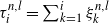
$ \tau^{n,l}_i = \sum_{k=1}^{i} \xi^{n,l}_k $
: time of the ith arrival to the lth queue. -
•
$ \eta^{n,l}_i $
: ith service time in the lth queue. -
•
$ s^{n,l}_i $
: ith switchover time from the lth queue.



We assume that the sequences
 $ \bigl\{ \xi^{n,l}_k,\, k \in \mathbb{N} \bigr\} $
,
 $ \bigl\{ \eta^{n,l}_k,\, k \in \mathbb{N} \bigr\} $
, and
 $ \bigl\{ s^{n,l}_k,\, k \in \mathbb{N} \bigr\} $
are independent and identically distributed for each
 $ l \in \{1,2\} $
. For the expected values of these random variables, we have
 \begin{gather*} \lambda^n_l=\dfrac{1}{\mathbb{E}\xi^{n,l}_1}, \quad \mu^n_l=\dfrac{1}{\mathbb{E}\eta^{n,l}_1}, \quad d^{n}_l=\mathbb{E}s^{n,l}_1, \quad \rho^n_l=\dfrac{\lambda^{n}_{l}}{\mu^{n}_l}, \\ \rho^n=\rho^n_1+\rho^n_2, \quad \sigma^n_l=\sqrt{\mathbb{E}\bigl(\eta^{n,l}_1-\rho^n_l \cdot \xi^{n,l}_1 \bigr)^2}.\end{gather*}
Let
 \begin{equation}V^{n}(t) = \dfrac{1}{\sqrt{n}} U^n_{nt}, \quad t \geq 0,\end{equation}
where
 $ U^n_t $
denotes the total unfinished work in the nth system at time t. It is assumed that the initial unfinished work
 $ U^n_0 $
is independent of the sequences
 $ \bigl\{ \xi^{n,l}_k,\, k \in \mathbb{N} \bigr\} $
,
 $ \bigl\{ \eta^{n,l}_k,\, k \in \mathbb{N} \bigr\} $
, and
 $ \bigl\{ s^{n,l}_k,\, k \in \mathbb{N} \bigr\} $
for
 $ l \in \{1,2\} $
.
Theorem 1 of [Reference Coffman, Puhalskii and Reiman8] establishes that the scaled total unfinished work (4.1) in the two-queue polling system can be approximated in the heavy-traffic regime by a Bessel process with negative constant drift. It turns out that this heavy-traffic approximation in the non-fractional case can be naturally extended to the fractional case.
Let
 \begin{equation}V^{n}_{\alpha}(t) = V^n(E(t)), \quad V_{\alpha}(t) = V(E(t)), \quad \alpha \in ( 0, 1 ),\end{equation}
where
 $ V = \{V(t),\, t \geq 0\} $
is the solution of the stochastic differential equation
 \[{\mathrm{d}} V(t) = \biggl( c + \dfrac{d}{V(t)} \biggr) \,{\mathrm{d}} t + \sigma\, {\mathrm{d}} B(t),\]
and E(t) is the inverse of an
 $ \alpha $
-stable subordinator as defined in (3.1), assumed to be independent of the processes
 $ V^n $
and V.
Theorem 4.1. Assume that
 $V^n(0) \Rightarrow V_0$
for some non-negative random variable
 $V_0$
. Suppose
 \begin{equation*}\lambda^n_l \to \lambda_l, \quad \mu^n_l \to \mu_l, \quad \sigma^n_l \to \sigma_l, \quad d^n_l \to d_l, \quad n \to \infty,\end{equation*}
and define
 \begin{equation*}\sigma^2=\lambda_1 \sigma^2_1 + \lambda_2 \sigma^2_2 >0, \quad \rho_l=\lambda_l/\mu_l, \quad l \in \{1,2\}, \quad d=\rho_1 \rho_2(d_1+d_2).\end{equation*}
Under the heavy traffic condition
 \begin{equation*}\sqrt{n}(\rho^n-1) \to c, \quad n \to \infty\end{equation*}
and the Lindeberg conditions
 \begin{equation*}\lim_{n \to \infty}\mathbb{E}\bigl(\xi^{n,l}_1\bigr)^2 \cdot 1_{\{\xi^{n,l}_1>\epsilon \sqrt{n}\}}=\lim_{n \to \infty}\mathbb{E}\bigl(\eta^{n,l}_1\bigr)^2 \cdot 1_{\{\eta^{n,l}_1>\epsilon \sqrt{n}\}}=\lim_{n \to \infty}\mathbb{E}\bigl(s^{n,l}_1\bigr)^2 \cdot 1_{\{s^{n,l}_1>\epsilon \sqrt{n}\}}=0,\end{equation*}
we have
 \begin{equation*}V^n_{\alpha} \Rightarrow V_{\alpha}, \quad n \to \infty\end{equation*}
in the Skorokhod space
 $\mathbb{D}([0,\,+\infty))$
equipped with the
 $J_1$
topology.
Proof. Under the conditions of the theorem, we have
 \begin{equation*}V^n \Rightarrow V, \quad n \to \infty\end{equation*}
in the Skorokhod space
 $\mathbb{D}([0,\,+\infty))$
with the
 $J_1$
topology (see [Reference Coffman, Puhalskii and Reiman8, Theorem 1]). Since the inverse
 $\alpha$
-stable subordinator
 $(E(t), \, t \geq 0)$
is a.s. continuous, non-decreasing, and independent of both
 $V^n$
and V, by classical arguments [Reference Whitt35] we have the desired convergence
 \begin{equation*}V^n_{\alpha} \Rightarrow V_{\alpha}, \quad n \to \infty\end{equation*}
in the Skorokhod space
 $\mathbb{D}([0,\,+\infty))$
with
 $J_1$
topology.
The idea behind the random time change in the processes (4.2) via the inverse of the
 $\alpha$
-stable subordinator is as follows. If the server in the aforementioned polling system malfunctions and stops working for random periods of time, then the total unfinished work remains the same until the server is repaired and new customers are allowed to enter the system.
The parameter
 $\alpha$
controls the length of the malfunction periods in the following way.
-
• Smaller values of
$\alpha$
correspond to longer malfunction periods, i.e. extended intervals during which the total unfinished work remains constant. -
• Larger values of
$\alpha$
correspond to shorter malfunction periods, i.e. brief intervals during which the total unfinished work remains constant. -
• Setting
$\alpha=1$
recovers the classical result of [Reference Coffman, Puhalskii and Reiman8, Theorem 1].


This behavior is further illustrated by simulated sample paths of the fractional and non-fractional Bessel processes (see Figure 1). The simulation is based on a standard approach for simulating time-changed stochastic models via inverse subordinators (see e.g. [Reference Magdziarz, Weron and Weron24]).
Sample paths of the non-fractional (a) and fractional (b) Bessel processes with parameters
 $\mu=-1$
,
 $\nu=0.5$
, and
 $\alpha=0.7$
, based on 10 000 points and initial state
 $X_0=0.4$
.

This means that the heavy traffic regime with random malfunction times can be modeled by stochastic process
 $V_{\alpha}=\{\sigma X_{\alpha}(t), \, t \geq 0\}$
, where
 $X_{\alpha}(t)$
is defined by (3.3) and the corresponding parameters from (2.1) are given by
 \begin{equation*}\mu=\dfrac{c}{\sigma}, \quad \nu=\dfrac{d}{\sigma^2}-\dfrac{1}{2}.\end{equation*}
Therefore one can exploit the spectral representation result in Theorem 3.1 to compute the asymptotic distributional properties of the two-queue polling model with exhaustive service and possible random malfunction times.
Under the assumptions of Theorem 4.1, and for any real-valued continuous function f, the well-known heavy traffic averaging principle (HTAP) is valid (see [Reference Coffman, Puhalskii and Reiman8, Theorem 2.2]):
 \begin{equation*}\int_{0}^{t}f(V^{n,l}_s)\,{\mathrm{d}} s \Rightarrow \int_{0}^{t}\int_{0}^{1}f(u V_s)\,{\mathrm{d}} u \,{\mathrm{d}} s, \quad n \to \infty.\end{equation*}
It turns out that the same reasoning used in the previous theorem extends the HTAP to the fractional model as well (FHTAP):
 \begin{equation*}\int_{0}^{t}f(V^{n,l}_{\alpha, s})\,{\mathrm{d}} s \Rightarrow \int_{0}^{t}\int_{0}^{1}f(u V_{\alpha, s})\,{\mathrm{d}} u \,{\mathrm{d}} s, \quad n \to \infty.\end{equation*}
In a similar manner one can show FHTAP for the sojourn times
 $W_{\alpha, t}(i)$
at queue
 $i \in \{1,2\}$
:
 \begin{equation*}\int_{0}^{t }f(Y^{n, i}_{\alpha, s})\,{\mathrm{d}} s\Rightarrow\int_{0}^{t}\int_{0}^{1}f\biggl (\dfrac{1-\rho_i}{\rho_1 \rho_2} u V_{\alpha, s}\biggr)\,{\mathrm{d}} u \,{\mathrm{d}} s, \quad n \to \infty,\end{equation*}
with
 $Y^{n, i}_{\alpha, s}=W^{n}_{\alpha, ns}(i)/\sqrt{n}, \, 0 \leq s \leq 1$
(see [Reference Coffman, Puhalskii and Reiman8, (1.2)] for the non-fractional case).
First we illustrate that in the stationary setting, fractional and non-fractional models lead to the same limiting mean values. Let
 $V_0$
be distributed according to the stationary gamma density (2.4). According to the HTAP, for
 $f(x)=x$
the limiting mean sojourn time of queue
 $i\in\{1,2\}$
can be approximated by
 \begin{align*}\mathbb{E}\biggl[\dfrac{1}{t}\int_0^t \int_0^1f\biggl(\dfrac{1-\rho_i}{\rho_1\rho_2}u\,V_s\biggr)\,{\mathrm{d}} u\,{\mathrm{d}} s\biggr]&=\dfrac{1}{t}\int_0^t\dfrac{1-\rho_i}{\rho_1\rho_2}\,\mathbb{E}V_s\,{\mathrm{d}} s \\&=\dfrac{1-\rho_i}{\rho_1\rho_2}\,\mathbb{E}V_0 \\&=-\dfrac{1-\rho_i}{\rho_1\rho_2}\,\dfrac{\nu+1}{\mu}.\end{align*}
The same conclusion holds for the fractional model. Although the time-changed process is not strictly stationary, if it is initialized according to the stationary distribution (2.4), its mean remains constant in time (in order to see this, average the identity (3.21) according to the stationary distribution). Consequently, the limiting mean sojourn times predicted by the HTAP coincide for the fractional and non-fractional models.
In the non-stationary setting, we illustrate the effect of fractional dynamics by numerically comparing the time evolution of conditional expectations and corresponding transition densities for the fractional and non-fractional queue diffusion approximations. Specifically, we exploit the obtained spectral representations (3.19) and (3.21) to compute the conditional expectations and transition densities of the Bessel process and its fractional counterpart, starting from a fixed initial state. We employ appropriate truncation of both the discrete series and the continuous spectral integral. In particular, Figures 2 and 3 use the first five terms of the discrete series, with the continuous spectral integral truncated at
 $\lambda=20$
. Recall that the discrete-series terms decay as
 ${\mathrm{O}} (n^{-3})$
(Lemma 3.1), so a few terms capture the sum to high precision, while the continuous-spectrum integrand decays as
 ${\mathrm{O}} (\lambda^{-3/2})$
as
 $\lambda\to\infty$
(Lemma 3.2). For example, extending the cutoff from
 $\lambda=20$
to
 $\lambda=100$
alters the integral by less than
 $1.5\times10^{-3}$
at the smallest plotted times, where the tail is heaviest. Consequently, all displayed quantities are accurate to at least two decimal places.
Graph of the conditional expectation
 $\mathbb{E}[X_{\alpha}(t) \mid X_{\alpha}(0)=1]$
for
 $0 \le t \le 10$
,
 $\alpha \in \{0.6, 0.8, 1\}$
, with parameters
 $\mu=-1$
and
 $\nu=0.5$
.

Transition density
 $p(x, t;\,y)$
(a) and fractional transition density
 $p_{\alpha}(x, t;\,y)$
(b) for Bessel process with parameters
 $\mu=-1, \nu=0.5$
,
 $\alpha=0.7$
and
 $y=1$
.

Figure 2 displays the convergence of the conditional expectation
 $\mathbb{E}[X_{\alpha}(t)\mid X_{\alpha}(0)=1]$
to the stationary mean (equal to
 $1.5$
for the chosen parameters) for different values of the fractional parameter
 $\alpha$
. The case
 $\alpha=1$
corresponds to the classical (non-fractional) model and exhibits the fastest convergence. Smaller values of
 $\alpha$
, which reflect heavy-tailed interruptions in the underlying time change, lead to a slower approach to stationarity. Even at relatively large times, the fractional models exhibit a significantly slower convergence to stationarity. For instance, at
 $t=30$
we obtain numerically
 \begin{align*}\mathbb{E}[X_{0.6}(30)\mid X_{0.6}(0)\,=\,1]&\approx 1.44, \\\mathbb{E}[X_{0.8}(30)\mid X_{0.8}(0)\,=\,1]&\approx 1.48, \\\mathbb{E}[X_{1}(30)\mid X_{1}(0)\,=\,1]&\approx 1.5,\end{align*}
illustrating that smaller values of
 $\alpha$
lead to a substantially slower approach to the stationary mean.
The major difference between the two models lies in the rate at which they approach the steady state. According to [Reference Linetsky23], the non-fractional model converges to the steady state exponentially fast, with decay parameter
 \begin{equation*}\delta =\left\{\begin{aligned}&\dfrac{\mu^2}{2} \biggl( 1 - \biggl( \dfrac{\nu + {\frac{1}{2}}}{\nu + \frac{3}{2}} \biggr)^2 \biggr), && \nu > -\tfrac{1}{2}, \\&\dfrac{\mu^2}{2}, && -1 < \nu < - \tfrac{1}{2}.\end{aligned}\right.\end{equation*}
More precisely,
 \begin{equation*}\delta \,:\!=\, \sup \{ \beta \geq 0 \colon p(x,t;\,y) - \pi(x) = {\mathrm{O}}({\mathrm{e}}^{-\beta t}) \text{ for all } y \in S \},\end{equation*}
where we assume
 $\mu<0$
and the stationary density
 $\pi(\!\cdot\!)$
is given by (2.4).
This behavior follows from the spectral structure and the corresponding spectral representation (2.11) of the transition density of the Bessel process. The temporal dependence enters through exponential factors
 ${\mathrm{e}}^{-\lambda t}$
, where
 $\lambda$
belongs either to the discrete spectrum (2.5) or to the essential spectrum (2.7). In particular, if
 $-1 < \nu < -\frac{1}{2}$
, the discrete spectrum consists only of
 $\lambda_0=0$
, while the lowest point of the essential spectrum is
 $\mu^2/2$
. On the other hand, if
 $\nu > -\frac{1}{2}$
, the smallest positive eigenvalue is
 \begin{equation*}\lambda_1 = \dfrac{\mu^2}{2} \biggl( 1 - \biggl( \dfrac{\nu + {\frac{1}{2}}}{\nu + \frac{3}{2}} \biggr)^2 \biggr).\end{equation*}
Recall that the fractional Bessel process is obtained via a stochastic time change of the classical Bessel process, which is reflected in the spectral representation given in Theorem 3.1. In this case, the exponential decay is replaced by a much slower decay governed by the Mittag–Leffler function
 $\mathcal{E}_{\alpha}(\! -\lambda t^{\alpha})$
, which is monotone decreasing. Since the spectral representations of the fractional and non-fractional models differ only in the temporal component, the above arguments can be repeated to conclude that the fractional Bessel process approaches the steady state with polynomial (power-law) decay with exponent
 $\alpha$
. More precisely,
 \begin{align*}&\sup \{ \beta \geq 0 \colon p_{\alpha}(x,t;\,y) - \pi(x) = {\mathrm{O}}(\mathcal{E}_{\alpha}(\! -\beta t^{\alpha})) \text{ for all $ y \in S$} \} \\&\quad =\left\{\begin{array}{ll} \dfrac{\mu^2}{2} \biggl( 1 - \biggl( \dfrac{\nu + {\frac{1}{2}}}{\nu + \frac{3}{2}} \biggr)^2 \biggr), & \quad \nu \gt -\tfrac{1}{2}, \\ \dfrac{\mu^2}{2}, & \quad -1 \lt \nu\lt - \tfrac{1}{2}.\end{array}\right.\end{align*}
Finally, recall that
 \begin{equation*}\mathcal{E}_{\alpha}(\! -\lambda t^{\alpha}) \sim \dfrac{1}{\Gamma(1-\alpha)\lambda t^{\alpha}},\quad t \to \infty.\end{equation*}
Figure 3 further illustrates the observed difference in the rates of convergence to the steady state.
Acknowledgement
I am grateful to the anonymous referees for several suggestions that improved the presentation of the manuscript.
Funding information
This work was supported by the Croatian Science Foundation under the project Scaling in Stochastic Models (HRZZ-IP-2022-10-8081).
Competing interests
There were no competing interests to declare which arose during the preparation or publication process of this article.
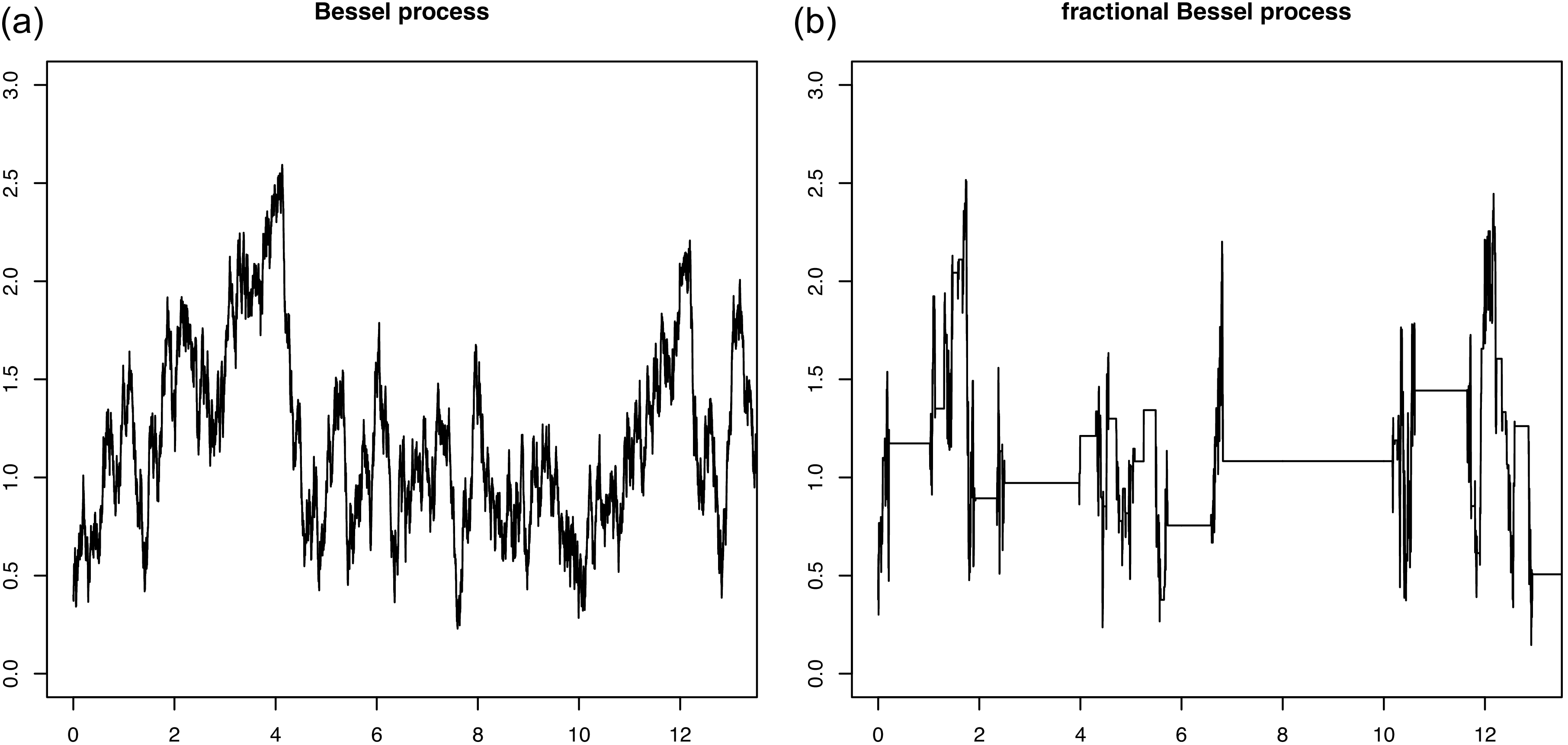
 μ=−1
 ν=0.5
 α=0.7
 X0=0.4
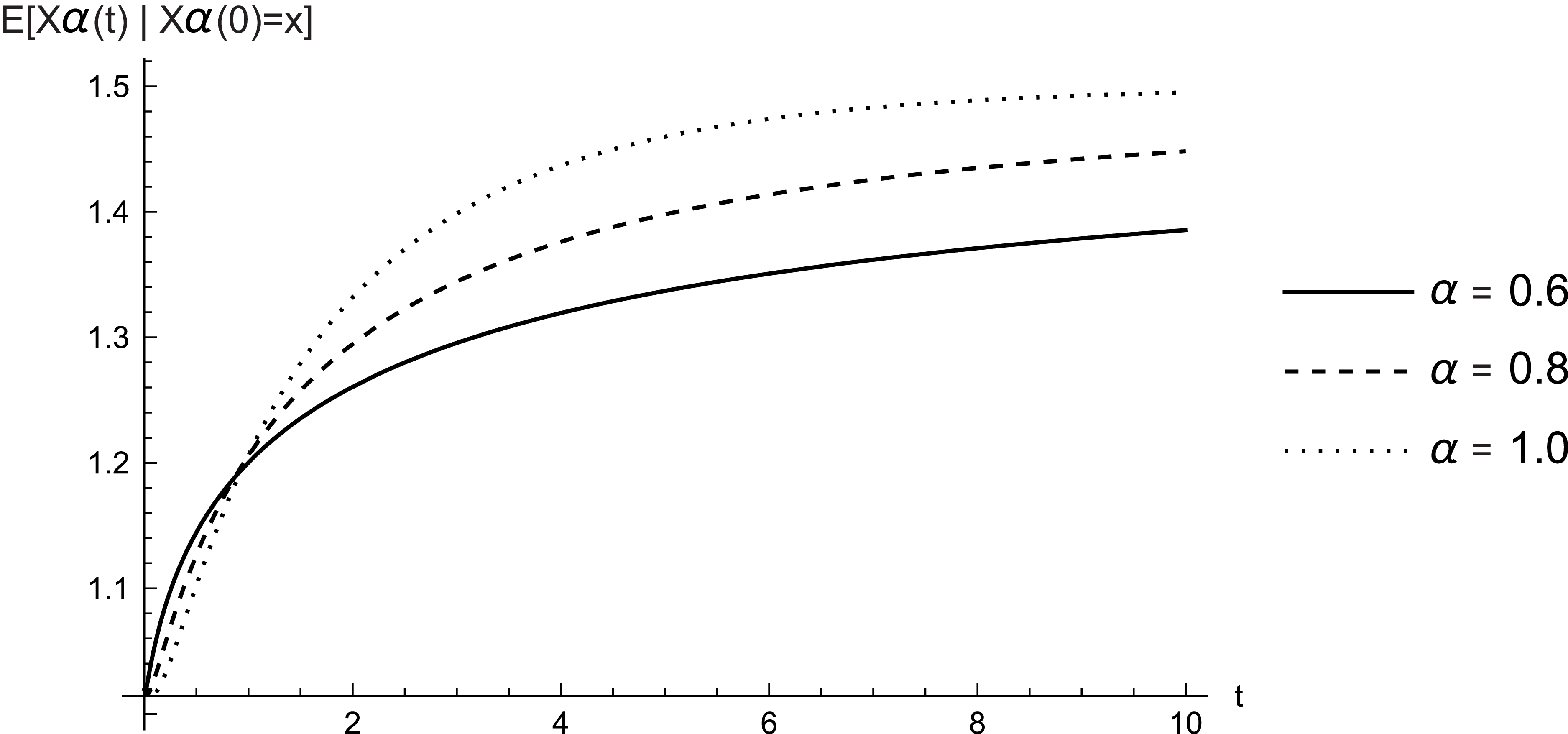
 E[Xα(t)∣Xα(0)=1]
 0≤t≤10
 α∈{0.6,0.8,1}
 μ=−1
 ν=0.5
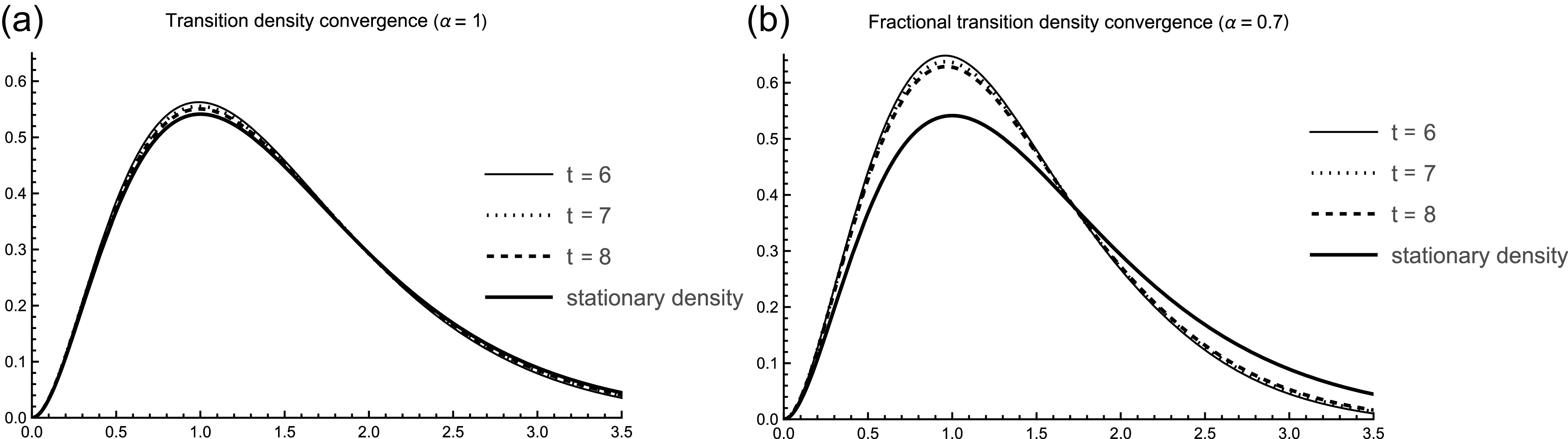
 p(x,t;y)
 pα(x,t;y)
 μ=−1,ν=0.5
 α=0.7
 y=1


