



1. Introduction
A focal point in the study of permutations is the characterization of the average or distribution of certain statistics. The goal is to discover better data processing algorithms. The hope is that such statistics may recommend or disqualify certain sorting algorithms.
Several statistics on permutations are classic, e.g. the number of cycles, the number of inversions, or the number of ascents, among a few others. They have underlying classical combinatorial numbers, such as Stirling numbers and Eulerian numbers [Reference Flajolet and Sedgewick8, Reference Graham, Knuth and Patashnik9].
Our intention is to look at yet another permutation statistic to add to the repertoire of potentially useful tools in the design of efficient algorithms. We consider a statistic that counts the number of elements that are ‘close’ to their natural position in the sorted permutation in ascending order. The word ‘close’ here is captured in a prespecified parameter called k.
More precisely, we define the k-window statistic in the following way. Suppose
 $\Pi_n = (\pi_1, \ldots, \pi_n)$
is a given permutation of
 $[n] \, :\!= \, \{1,\ldots,n\}$
, with
 $\pi_i$
being the position of
 $i\in [n]$
in the permutation. For
 $0 \le k \le n-1$
, let
 $C_k(\Pi_n)$
be the number of elements in
 $\Pi_n$
that are at a distance no greater than k from their natural position (the natural position
 $\pi_i$
for i is i). In other words, we set
 \begin{align*}C_k (\Pi_n)= |\{i\colon |\pi_i -i|\le k\}|; \end{align*}
applied to a set
 $\mathcal A$
, the notation
 $|\mathcal A|$
is the cardinality or size of the set. For brevity, we drop
 $\Pi_n$
from the notation and simply write
 $C_{n,k}$
.
Another way to think of
 $C_{n,k}$
is to put a viewing window of width
 $2k+1$
centered at every position
 $i\in [n]$
, and add 1 to the count
 $C_{n,k}$
, for every i seen in its associated window. This suggests a name for the statistic. Let us call it the k-window statistic (a displacement of no more than k positions to the left or k positions to the right).
The 0-window statistic counts the number of fixed points in a permutation. This has been studied; see [Reference Barbour, Holst and Janson4, Example 3.4.2], for instance. To the best of our knowledge, the k-window statistic has not been considered much for other values of k, particularly for k growing with n. We look at the entire spectrum of k; the forthcoming analysis shows phase transitions in the asymptotic average, variance, and distribution of
 $C_{n,k}$
.
We focus on random permutations, where the randomness means that all permutations of [n] are equally likely. Indeed, a large class of data has ranks that are random permutations. For instance, the ranks of the observations in a sample of size n taken from any continuous distribution are almost surely in a random permutation of [n].
In what follows, we use the notation
 $\mathbf{1}_{\mathcal{E}}$
for the indicator of the event
 $\mathcal E$
. The k-window statistic can be represented as a sum of indicators:
 \begin{equation}C_{n,k} = \sum_{i=1}^n \mathbf{1}_{\{|\pi_i -i| \le k\}}.\end{equation}
The indicators involved are dependent. They are heterogeneous in the sense they are not identically distributed and the dependency between different pairs may not be the same. For instance, for
 $n=3$
, and
 $k=1$
, the two indicators
 $\mathbf{1}_{\{|\pi_1 -1| \le 1\}}$
and
 $\mathbf{1}_{\{|\pi_2 -2| \le 1\}}$
are uncorrelated, whereas the covariance between
 $\mathbf{1}_{\{|\pi_1 -1| \le 1\}}$
and
 $\mathbf{1}_{\{|\pi_3 -3| \le 1\}}$
is
 $\tfrac{1}{18}$
.
Consider an
 $n\times n$
matrix (which we call
 $\mathbf{A}_n$
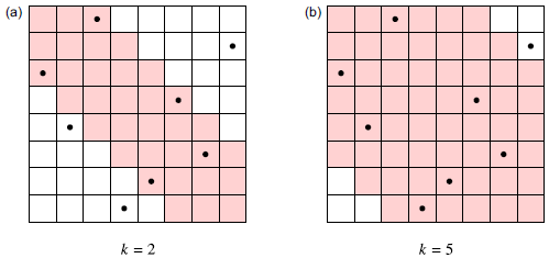
) with rows indexed by i and columns indexed by r, and filled with 1s and 0s. The 1s appear in a band around the main diagonal, where the absolute difference between i and r is at most k, and the rest of the entries in the matrix are 0s. Figure 1 shows the matrix
 $\mathbf{A}_8$
, with
 $k=2$
(windows of width 5 in (a)) and with
 $k=5$
(windows of width 11 in (b)). The positions containing 1 are colored pink.
The permutation
 $\boldsymbol{\Pi}_{8}=(3,8,1,6,2,7,5,4)$
represented as bullets in an
 $8\times8$
grid appearing at the positions
 $(i, \pi_{i})$
. The pink shaded cells satisfy
 $|i-j| \le k$
; (a)
 $k=2$
, (b)
 $k=5$
.

Suppose the permutation in the positional notation is
 \begin{align*}3 \quad 8 \quad 1 \quad 6 \quad 2 \quad 7 \quad 5 \quad 4. \end{align*}
The bullets in both grids show where the elements of this permutation are. For example, the element 1 appears in the third position in the permutation: cell (1, 3) receives a bullet and is seen in a window of width 5 (in the pink region in (a)), contributing 1 to
 $C_{8,2}$
. It is also seen in a window of length 11 (in the pink region in (b)), contributing 1 to
 $C_{8,5}$
. The element 5 appears at position 2 in the permutation, which is not in the pink area in (a), contributing 0 to
 $C_{8,2}$
, but is in the pink region in (b), contributing 1 to
 $C_{8,5}$
. For this permutation, we compute
 \begin{align*}C_{8,2} = 1+0 +1+1+0+1+1+0 = 5,\quad C_{8,5} = 1+0 +1+1+1+1+1+1 = 7. \end{align*}
2. The mean of the k-window statistic
We pin down the exact mean of
 $C_{n,k}$
, from which we can extract asymptotics and discern phases within.
Proposition 2.1. Let k be an integer between
 $0$
and
 $n-1$
. In a random permutation of
 $[n]$
, the average of the k-window statistic is
 \begin{align*}{\mathbb E}[C_{n,k}] = 2k + 1 - \frac kn (k +1). \end{align*}
Proof. Take expectations of (1.1) to get
 \begin{align*}{\mathbb E}[C_{n,k}] = \sum_{i=1}^n \sum_{r=1}^n \mathbf{1}_{\{|r -i| \le k\}}\, {\mathbb P}(\pi_i= r) = \dfrac 1 n\sum_{i=1}^n \sum_{r=1}^n \mathbf{1}_{\{|r -i| \le k\}}. \end{align*}
Here and throughout, we call the sum
 $\sum_{r=1}^n \mathbf{1}_{\{|r -i| \le k\}}$
by the name
 $x_{n,i,k}$
. In view of edge effects, we evaluate
 $x_{n,i,k}$
piecewise and deal with cases. Thus
 $x_{n,i,k}$
counts the 1s across row i in this matrix.
The case
 $0\le k < n/2$
. We find
 \begin{align*}x_{n,i,k} = \begin{cases} k+i , &\text{for $ i = 1,\ldots,k$,}\\[3pt] 2k+1 , & \text{for $ i = k+1, \ldots, n-k$,}\\[3pt] k+1+ n-i, &\text{for $ i = n-k+1, \ldots,n$.} \end{cases} \end{align*}
It follows that
 \begin{align}\sum_{i=1}^n x_{n,i,k} &= \sum_{i=1}^k (k+i) + \sum_{i=k+1}^{n-k} (2k+1) + \sum_{i=n-k+1}^n (k+1+n-i)\nonumber \\[3pt] &= (2k+1)n - k(k+1). \end{align}
The case
 $k \ge n/2$
. We find
 \begin{align*}x_{n,i,k} = \begin{cases} k+i , &\text{for $ i = 1,\ldots,n-k-1$,}\\[3pt] n , & \text{for $ i = n-k, \ldots, k+1$,}\\[3pt] k+1 +n-i , &\text{for $ i = k+2, \ldots,n$.} \end{cases} \end{align*}
It follows that
 \begin{align*}\sum_{i=1}^n x_{n,i,k} &= \sum_{i=1}^{n-k-1} (k+i) + \sum_{i=n-k}^{k+1} n + \sum_{i=k+2}^n (k+1+n-i)\nonumber \\[3pt] &= (2k+1)n - k(k+1),\end{align*}
which is the same expression as the counterpart in the case
 $k < n/2$
. In either case, we get
 \begin{equation*}{\mathbb E}[C_{n,k}] = \dfrac 1 n\sum_{i=1}^n x_{n,i,k} = (2k+1) - \dfrac k n(k+1).\end{equation*}
2.1. Phases in the average of
 $C_{n,k}$

We keep in mind that k may depend on n. We write
 \begin{align*}k = k_n = \alpha n +g_n, \end{align*}
where
 $g_n$
is
 ${\mathrm{o}} (n)$
. Depending on context, we simply write k when k is fixed, or appears in huge formulas, or when suggested by aesthetics. In other places, where convergence is discussed, it is preferable to write
 $k_n$
.
The case
 $\alpha=0$
covers slowly growing (sublinear) k, such as when k is a fixed number (in which case
 $g_n = k$
), or a case such as
 $k_n = 0 + g_n = \lfloor 6n^{3/4} + \pi \sqrt n + e \ln n -5 \rfloor$
.
To determine the asymptotics of
 ${\mathbb E}[C_{n,k}]$
, we use the
 $\Theta$
notation, which specifies the exact growth rate of a function. The notation
 $\Theta$
is popular in the literature of computer science. For a function
 $g_n$
, if there exist two real positive constants
 $c_1$
and
 $c_2$
, and a natural number
 $n_0$
, such that
 \begin{align*}c_1 |h_n| \le |g_n| \le c_2 |h_n|\quad \text{for all $ n \ge n_0$,} \end{align*}
we say that
 $g_n$
is of the same exact order of growth as the function
 $h_n$
and write this as
 $g_n = \Theta (h_n)$
. Consider first the regime in which
 $\alpha \in [0,1)$
. Plugging the representation of
 $k_n$
into the exact expression of Proposition 2.1, we get
 \begin{align*}{\mathbb E}[C_{n,k}] &= 2(\alpha n + g_n) + 1 - \dfrac {\alpha n + g_n} n (\alpha n + g_n +1) \\[3pt] &=\alpha (2-\alpha) n + 2(1-\alpha)g_n + 1-\alpha -\dfrac {g^2_n + g_n} n .\end{align*}
The order of
 $g^2_n/n$
is always
 ${\mathrm{o}} (g_n)$
. Hence, for k in the sublinear regime (where
 $\alpha=0)$
, we have
 \begin{align*}{\mathbb E}[C_{n,k}] = 2g_n + 1 + \Theta\biggl(\dfrac {g^2_n} n\biggr); \end{align*}
the average of the k-window statistic is also in a sublinear phase.
In the linear regime
 $k_n = \alpha n + g_n$
the function
 $g_n$
is
 ${\mathrm{o}} (n)$
, and if
 $\alpha=1$
this function is negative. With
 $\alpha\in (0, 1]$
, the average comes up into a linear phase too:
 \begin{equation}{\mathbb E}[C_{n,k}] = \alpha (2-\alpha) n + 2(1-\alpha)g_n + 1-\alpha - \Theta\biggl(\dfrac {g^2_n} n\biggr).\end{equation}
It is evident from the asymptotic approximation that we get a sublinear (in n) average for the k-window statistic, for
 $\alpha =0$
, then the average transitions into a linear phase, when
 $\alpha$
is in (0, 1].
In the linear phase, the coefficient of linearity in the average increases with rising
 $\alpha$
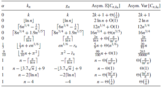
. Table 1 shows the asymptotics of the average of
 $C_{n,k_n}$
for some selected
 $k_n$
functions. In the table, the functions
 $r_n$
and
 $\tilde r_n$
are corrections with values in [0, 1) that appear upon removing the floors.
Asymptotics for some selected
 $k_n$
functions.

Table 1 Long description
A table with 10 rows and 5 columns. The columns are labeled k_n, g_n, Asym., E[C_n,k_n], and Asym. Var [C_n,k_n]. The table presents various functions and their asymptotic behaviors. Row 1: k_n is k, g_n is k, Asym. is 2k + 1 + Θ(1/n), E[C_n,k_n] is 2k + 1, and Asym. Var [C_n,k_n] is 2k + 1. Row 2: k_n is ⌊ln n⌋, g_n is ⌊ln n⌋, Asym. is 2ln n + O(1), E[C_n,k_n] is 2ln n, and Asym. Var [C_n,k_n] is 2ln n. Row 3: k_n is ⌊6n^(1/4) - (1/n)⌋, g_n is ⌊6n^(1/4) - (1/n)⌋, Asym. is 12n^(1/4) + O(1), E[C_n,k_n] is 12n^(1/4), and Asym. Var [C_n,k_n] is 12n^(1/4). Row 4: k_n is ⌊8n^(3/4) + 1.9n^(3/5)⌋, g_n is ⌊8n^(3/4) + 1.9n^(3/5)⌋, Asym. is 16n^(3/4) + Θ(n^(3/5)), E[C_n,k_n] is 16n^(3/4), and Asym. Var [C_n,k_n] is 16n^(3/4). Row 5: k_n is ⌊(n/ln n)⌋, g_n is ⌊(n/ln n)⌋, Asym. is (2n/(ln n)) + Θ((n/(ln^2 n))), E[C_n,k_n] is (2n/(ln n)), and Asym. Var [C_n,k_n] is (2n/(ln n)). Row 6: k_n is ⌊(1/3)n + en^(1/6)⌋, g_n is en^(1/6) - r_n, Asym. is (5/9)n + Θ(n^(1/6)), E[C_n,k_n] is (5/9)n, and Asym. Var [C_n,k_n] is (20/81)n. Row 7: k_n is ⌊(9/10)n + π^2⌋, g_n is π^2 - r_n, Asym. is (99/100)n + Θ(1), E[C_n,k_n] is (99/100)n, and Asym. Var [C_n,k_n] is (263/30000)n. Row 8: k_n is n - ⌊(n/ln n)⌋, g_n is -(n/ln n), Asym. is n - Θ((n/(ln n))), E[C_n,k_n] is n, and Asym. Var [C_n,k_n] is Θ((n/(ln^2 n))). Row 9: k_n is n - ⌊3.7√(n)⌋ + 9, g_n is -⌊3.7√(n)⌋ + 9, Asym. is n - Θ(1), E[C_n,k_n] is n, and Asym. Var [C_n,k_n] is Θ(1). Row 10: k_n is n - 2⌊ln n⌋, g_n is -2⌊ln n⌋, Asym. is n - Θ((ln^2 n)/n), E[C_n,k_n] is n, and Asym. Var [C_n,k_n] is Θ((ln^2 n)/n). Row 11: k_n is n - 4, g_n is -4, Asym. is n - Θ(1/n), E[C_n,k_n] is n, and Asym. Var [C_n,k_n] is Θ(1/n).
Remark 2.1. There is no limit to how bizarre the function
 $k_n$
can be. For example, one could think of a function alternating between high and low values, such as
 \begin{align*}k_n = \begin{cases} 1, & \text{for odd} \ \textit{n},\\[3pt] \lfloor \sqrt n \, \rfloor, & \text{for even} \ \textit{n}. \end{cases} \end{align*}
Such a concocted sequence is not likely to appear in practice, and therefore is of no interest. We confine our attention to functions
 $k_n$
that are constants or driven by a dominant naturally growing function.
3. The variance of the k-window statistic
Toward the exact variance of
 $C_{n,k}$
, we begin with its second moment. Squaring the stochastic equation (1.1), we get
 \begin{align*}C_{n,k}^2 &= \sum_{1 \le i, j\le n} \mathbf{1}_{\{|\pi_i -i| \le k\}} \mathbf{1}_{\{|\pi_j -j| \le k\}} \end{align*}
 \begin{align} &= \sum_{i=1}^n \mathbf{1}_{\{|\pi_i -i| \le k\}} + \sum_{\substack{1 \le i, j\le n\\[3pt] i \not = j}} \mathbf{1}_{\{|\pi_i -i| \le k\}} \, \mathbf{1}_{\{|\pi_j -j| \le k\}} \nonumber\\[3pt] &= C_{n,k} + \sum_{\substack{1 \le i, j\le n\\[3pt] i \not = j}} \mathbf{1}_{\{|\pi_i -i| \le k\}} \, \mathbf{1}_{\{|\pi_j -j| \le k\}}. \end{align}
Proposition 3.1. Let k be an integer between
 $0$
and
 $n-1$
. In a random permutation of
 $[n]$
, the variance of the k-window statistic is
 \begin{align*}\operatorname{Var}[C_{n,k}] = \begin{cases}(3(2k + 1)n^3 - 3(5k^2 + 5k + 1)n^2 \\[3pt] \quad {} + 4k(k+1)(2k+1) n + 3k^2(k + 1)^2) /(3n^2(n - 1)), & \textit{for} \ \text{ $ 0 \le k < n/2$,}\\[3pt] ((n - k - 1)(n - k)\\[3pt] \quad {} \times (2n^2 - (2k + 1)n + 3k (k + 1)) /(3n^2(n - 1)), & \textit{for} \ \text{$ n/2\le k < n$.}\end{cases}\end{align*}
Proof. Take expectations of (3.1), noting that for distinct i and j, the positions
 $\pi_i$
and
 $\pi_j$
are distinct, and the joint distribution of
 $(\pi_i,\pi_j)$
is uniform over
 $[n]\times [n] -\{(i,i) \colon i = 1, \ldots, n \}$
. This yields
 \begin{align*}{\mathbb E}\big[C_{n,k}^2\big] = {\mathbb E}[C_{n,k}] + \dfrac 1 {n(n-1)} \sum_{\substack{1\le i,j,r,s \le n\\[3pt] i\not= j, r\not = s}} \mathbf{1}_{\{|r -i| \le k\}}\, \mathbf{1}_{\{|s-j| \le k\}}. \end{align*}
For economy of space, we introduce the notation
 $\mathbf{J}_{p,q,k} = \mathbf{1}_{\{|p -q| \le k\}}$
to write the last relation as
 \begin{align*}{\mathbb E}\big[C_{n,k}^2\big] &= {\mathbb E}[C_{n,k}] + \dfrac 1 {n(n-1)} \sum_{\substack{1\le i,j,r,s \le n \\[3pt] i \not = j, r \not = s}}\mathbf{J}_{r,i,k}\, \mathbf{J}_{s,j,k} \\[3pt] &= {\mathbb E}[C_{n,k}] + \dfrac 1 {n(n-1)} \!\left(\rule{0pt}{21pt}\right.\! \sum_{\substack{1\le i,j,r,s \le n \\[3pt] r \not = s}} \mathbf{J}_ {r,i,k}\, \mathbf{J}_{s,j,k} - \sum_{\substack{1\le i,r,s \le n\ r \not = s}} \mathbf{J}_{r,i,k}\,\mathbf{J}_{s,i,k}\!\left.\rule{0pt}{21pt}\right)\!\\[3pt] &\, =\!: \, {\mathbb E}[C_{n,k}] + \dfrac 1 {n(n-1)}( L_{n,k} - M_{n,k}) ,\end{align*}
where
 $L_{n,k}$
and
 $M_{n,k}$
are the two four-fold sums in the penultimate line, defined in their order of appearance.
We have an exact expression for
 ${\mathbb E}[C_{n,k}]$
from Proposition 2.1. The evaluation of these four-fold sums requires a very lengthy computation that can be distracting; we only give the result here and relegate the detailed derivation to the appendix. We have
 \begin{align*}L_{n,k} &= \begin{cases} (2k+1)((2k+1) n^2 - (2k^2 + 4k +1)n)\\[3pt] \quad{} + \tfrac{1}{3} k(k+1)(3k^2+13k+5), & \text{for $ 0 \le k < n/2$,}\\[3pt] \tfrac{1}{3} n^3 + 2k(2k+1)n^2 - ( 4k^3 +6k^2 +2k + \tfrac{1}{3}) n \\[3pt] \quad {}+ \tfrac{1}{3} k(k+1) (3k^2 +5k +1), & \text{for $ n/2 \le k < n$,}\\[3pt] \end{cases}\end{align*}
and
 \begin{align*}M_{n,k} &= \begin{cases} 2k(2k+1)n - \tfrac{2}{3} k(k + 1)(5k + 1), & \text{for $ 0 \le k < n/2$,}\\[3pt] - \tfrac{1}{3} n^3 + (2k +1) n^2 - \tfrac{2}{3} (3k+1) n - \tfrac{2}{3} k(k^2-1), &\text{for $ n/2\le k < n$.} \end{cases}\end{align*}
Assembling all the elements and simplifying, we get
 \begin{align*}{\mathbb E}\big[C_{n,k}^2\big] = \begin{cases} (6(k+1)(2k+1) n^2 - 3(4k^3 +15k^2 +11k + 2)n \\[3pt] \quad {}+ k(k+1)(3k^2+23k +10)) /(3n(n - 1)), &\text{for $ 0 \le k < n/2$,}\\[3pt] (2 n^3 + 6k (2k+1) n^2 -( 12k^3+21k^2+9k+2)n\\[3pt] \quad {} +k(k+1)(k+2) (3k+1)) /(3n(n - 1)), & \text{for $ n/2\le k < n$.}\end{cases}\end{align*}
The variance follows from the computation of
 ${\mathbb E}\bigl[C_{n,k}^2\bigr] - {\mathbb E}^2[C_{n,k}]$
and further algebraic simplification yielding the stated expression.
3.1. Phases in the variance of
$C_{n,k}$

We can now identify phases in the variance. Let
 $k=k_n = \alpha n + g_n$
, with
 $g_n ={\mathrm{o}} (n)$
, as
 $n\to \infty$
. For
 $\alpha = 0$
, we have the asymptotic equivalent
 \begin{align*}\operatorname{Var}[C_{n,k}] \sim 2g_n + 1. \end{align*}
In contrast, for
 $0 < \alpha < \tfrac{1}{2}$
, the variance is in the linear phase
 \begin{align*}\operatorname{Var}[C_{n,k}] =\alpha\biggl(\alpha^3 + \dfrac 8 3 \alpha^2 - 5\alpha + 2\biggr) n + \Theta(g_n), \end{align*}
whereas for
 $\tfrac{1}{2} \le \alpha <1$
, the variance enters the linear phase
 \begin{align*}\operatorname{Var}[C_{n,k}] =\biggl(\alpha^4 - \dfrac 8 3\alpha^3 + 3\alpha^2 - 2\alpha + \dfrac 2 3\biggr)n + \Theta(g_n). \end{align*}
We note that at
 $\alpha = \tfrac{1}{2}$
, the linearity coefficients
 $\alpha \bigl(\alpha^3 + \tfrac{8}{3} \alpha^2 - 5\alpha + 2\bigr)$
and
 $\bigl(\alpha^4 - \tfrac{8}{3}\alpha^3 + 3\alpha^2 - 2\alpha + \tfrac{2}{3}\bigr)$
are both equal to
 $\tfrac{7}{48}$
, showing that the two linear phases meet smoothly at the seam line. Also, note that the coefficient of n is 0 at
 $\alpha =0$
and again at
 $\alpha = 1$
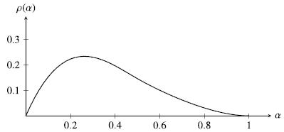
. Figure 2 shows a plot of
 $\rho (\alpha)$
, the coefficient of n in
 $\operatorname{Var}[C_{n,k}]$
, for
 $\alpha \in [0,1]$
.
The coefficient
 $\rho(\alpha)$
of n as a function of
 $\alpha$
.

The regime in which
 $\alpha =1$
offers its own twists. Within this regime,
 $k_n$
assumes the form
 $n+g_n$
, for some negative function
 $g_n = {\mathrm{o}} (n)$
. The exact variance in Proposition 3.1 in this regime degenerates into
 \begin{align*}\operatorname{Var}[C_{n,k}] &= \dfrac {\bigl(n^2 -\tfrac{4}{3} ng_n + g^2_n +\tfrac{2}{3} n -g_n \bigr)g_n(g_n - 1)}{n^2(n - 1)}\\[3pt] & \sim \dfrac {g^2_n}{n} \quad \text{as $ n\to\infty$.}\end{align*}
In this regime of extremely large windows, if the function
 $g_n$
grows at a rate faster than
 $\sqrt n$
(but remains
 ${\mathrm{o}} (n)$
, of course), we get a growing variance. At
 $g_n \sim c \sqrt n\,$
, the variance is asymptotic to
 $c^2$
. However, if
 $g_n ={\mathrm{o}} (\sqrt n\,)$
, the variance diminishes to 0 as
 $n\to\infty$
. Table 1 shows the asymptotics of the variance of
 $C_{n,k_n}$
for some selected
 $k_n$
functions.
4. Concentration
We use the notation
 $\buildrel {\mathbb P} \over \longrightarrow$
for convergence in probability, and
 $\buildrel \text{a.s.} \over \longrightarrow$
for convergence almost surely. In the regime where
 $\alpha =0$
, but
 $g_n$
is growing and the regime
 $0 < \alpha <1$
, the variance is small enough relative to the square of the mean, and this gives us a weak law of large numbers for the k-window statistic in the following way. According to the Chebyshev inequality, in the sublinear regime
 $k_n$
, with
 $g_n$
growing, for all
 $\varepsilon > 0$
, we have
 \begin{align*}{\mathbb P}(|C_{n,k}-{\mathbb E}[C_{n,k}]| >\varepsilon\, {\mathbb E}[C_{n,k}]) \le \dfrac {\operatorname{Var}[C_{n,k}]} {\varepsilon^2\, {\mathbb E}^2[C_{n,k}]} = \dfrac {\Theta(g_n)} {\Theta(g^2_n)}\to 0 \quad \text{as $ n \to\infty$.} \end{align*}
Hence, for
 $\alpha=0$
and growing
 $g_n$
, we have the convergence
 $C_{n,k}/{\mathbb E}[C_{n,k}]\buildrel {\mathbb P} \over \longrightarrow 1$
. Yet, we have
 ${\mathbb E}[C_{n,k}]/g_n \to 2$
. Combining these convergence relations, we get
 \begin{align*}\dfrac {C_{n,k}} {g_n} \buildrel {\mathbb P} \over \longrightarrow 2 \quad \text{as $ n \to\infty$.} \end{align*}
In the linear regime
 $k_n \sim\alpha n$
with
 $\alpha\in(0, 1)$
, we have
 ${\mathbb E}[C_{n,k}] \sim \alpha(2-\alpha) n$
, and
 $\operatorname{Var}[C_{n,k}] \sim \rho(\alpha) n$
. For all
 $\varepsilon > 0$
, we have
 \begin{align*}{\mathbb P}(|C_{n,k}-{\mathbb E}[C_{n,k}]| >\varepsilon\, {\mathbb E}[C_{n,k}]) = \dfrac {\Theta(n)} {\Theta(n^2)}\to 0 \quad \text{as $ n \to\infty$.} \end{align*}
Hence we have the convergence
 $C_{n,k}/{\mathbb E}[C_{n,k}]\buildrel {\mathbb P} \over \longrightarrow 1$
. Yet, we have
 ${\mathbb E}[C_{n,k}]/n\to \alpha(2-\alpha)$
. Combining these convergence relations, we get
 \begin{align*}\dfrac {C_{n,k}} n \buildrel {\mathbb P} \over \longrightarrow \alpha (2 -\alpha) \quad \text{as $ n \to\infty$.} \end{align*}
In the regime
 $\alpha=1$
, the Chebyshev bound
 $\operatorname{Var}[C_{n,k}] /(\varepsilon^2 {\mathbb E}^2[C_{n,k}])$
is
 $\Theta(g^2_n/n^3)$
. Hence we have the convergence
 $C_{n,k}/{\mathbb E}[C_{n,k}]\buildrel {\mathbb P} \over \longrightarrow 1$
. Yet, we have
 ${\mathbb E}[C_{n,k}]/n\to 1$
. Combining these convergence relations, we get
 \begin{align*}\dfrac {C_{n,k}} n \buildrel {\mathbb P} \over \longrightarrow 1 \quad \text{as $ n \to\infty$.} \end{align*}
If the Chebyshev bound is
 ${\mathrm{O}} (n^{-(1+\delta})$
, for some
 $\delta> 0$
, the probability on the left-hand side of Chebyshev’s inequality becomes summable. Via the Borel–Cantelli lemma, the convergence is upgraded to be almost sure. That is, in the regime
 $k_n = \alpha n - {\mathrm{O}} (n^{1-\delta/2})$
, for some
 $\delta > 0$
, we have
 $C_{n,k}/n\buildrel \text{a.s.} \over \longrightarrow 1$
. For instance, for
 $k_n = n - 5\lfloor n^{3/4}\rfloor$
, we get the bound
 $\Theta (n^{-3/2})$
in the Chebyshev inequality, with the conclusion that
 $C_{n,k} /n\buildrel \text{a.s.} \over \longrightarrow 1$
.
Remark 4.1. The regime of fixed k is excluded from this approach to the law of large numbers.
Remark 4.2. As in (2.2) and the concluding discussion before Remark 4.1, there is something special about the regime
 $\alpha=1$
. The presence of
 $1-\alpha=0$
in the formula (2.2) for
 ${\mathbb E}[C_{n,k}]$
eliminates the terms
 $2(1-\alpha) g_n$
and
 $1-\alpha$
before it gets down to the diminishing order
 $g_n^2/n$
.
5. The full spectrum of distributions
We denote the Poisson random variable with parameter
 $\lambda > 0$
by
 $\operatorname{Poi}( \lambda)$
, and denote the centered normal random variable with variance
 $\sigma^2$
by
 $\mathcal{N}(0,\sigma^2)$
, with cumulative distribution function
 ${\mathbb P}(\mathcal{N}(0,1) \le x) = \Phi(x)$
. We denote convergence in distribution by the symbol
 ${\buildrel \mathcal{D} \over \longrightarrow}$
. For the r-times falling factorial of a number y, we use Pochhammer’s symbol
 \begin{align*}(y) _r = y(y-1) \cdots (y-r +1). \end{align*}
The method of convergence of all falling factorial moments is used to establish convergence in distribution in the case of fixed k. In certain regimes, Bolthausen’s theorem [Reference Bolthausen6] is instrumental for establishing the rate of convergence to Gaussianity. It is one of several variations and improvements over the classic combinatorial central limit theorem by Hoeffding [Reference Hoeffding10]. For other improvements, see [Reference Barbour and Janson3] and [Reference Barbour, Holst and Janson4]. For the reader’s convenience, we give a statement of this theorem.
Theorem 5.1. (Bolthausen [Reference Bolthausen6].) Let
 $\mathbf{A}_n=(a_{i,j})$
be an
 $n\times n$
matrix of real numbers. Let
 \begin{align*}\mu_{\mathbf{A}_n} = n a_{..},\quad \sigma^2_{\mathbf{A}_n} =\dfrac 1 {n-1} \sum_{1\le i, j\le n} (a_{ij} - a_{i.} - a_{.j} + a..)^2, \end{align*}
where
 \begin{align*}a_{i.} = \dfrac 1 n \sum_{j=1}^n a_{ij}, \quad a_{.j} = \dfrac 1 n \sum_{i=1}^n a_{ij}, \quad a_{..} = \dfrac 1 {n^2} \sum_{1 \le i,j \le n} a_{ij}. \end{align*}
For a uniform random permutation
 $(\pi_1, \ldots, \pi_n)$
, we have
 \begin{equation}\sup_{x}\biggl(\biggl|{\mathbb P} \biggl(\dfrac{a_{i,\pi_n} - \mu_{\mathbf{A}_n}} {\sigma_{\mathbf{A}_n}} \le x\biggr) - \Phi(x)\biggr|\biggr)\le \dfrac K n \sum_{1\le i,j\le n} \biggl|\dfrac { a_{ij} - a_{i.} - a_{.j} + a_{..}} {\sigma _{\mathbf{A}_n}} \biggr|^3 ,\end{equation}
for some positive constant K.
We apply Theorem 5.1 to the specialized k-window matrix,
 $\mathbf{A}_n$
, described at the end of Section 1. Note that in the notation of the present paper,
 $a_{i.}$
is
 $x_{n,i,k}/n$
. For this specific matrix, its symmetry renders
 $a_{.j} = x_{n,j,k}/n$
too.
In certain regimes, the Chen–Stein method is the right tool. We use the version stated in [Reference Arratia, Goldstein and Gordon2] (proved in [Reference Arratia, Goldstein and Gordon1]). For a wider scope see [Reference Barbour, Holst and Janson4]. We state the theorem here for the reader’s convenience.
The theorem is based on bounding the total variation distance. For non-negative integer-valued random variables X and Y, let
 ${\mathbb P}_X$
and
 ${\mathbb Q}_Y$
be the measures specifying the distributions of X and Y over
 $\mathbb N \cup \{0\}$
. The total variation distance is defined as
 \begin{align*}d_{\textit{TV}}({\mathbb P}_X,{\mathbb Q}_Y)= \sup_{A \subseteq \mathbb N \cup \{0\}} |{\mathbb P}_X(A) - {\mathbb Q}_Y (A)|= \dfrac 1 2 \sum_{j=0}^\infty |{\mathbb P}_X(X=j) - {\mathbb Q}_Y( Y=j) |. \end{align*}
Many authors directly write
 $d_{\textit{TV}}(X,Y)$
for
 $d_{\textit{TV}}({\mathbb P}_X,\mathbb Q_Y)$
. We follow this simplifying convention, but it should be understood that the total variation distance is between probability laws, not between random variables. It is well known that convergence in total variation distance implies convergence in distribution.
Theorem 5.2. (Arratia, Goldstein, and Gordon [Reference Arratia, Goldstein and Gordon2].) Let
 $\mathcal{I}$
be an arbitrary index set, and for
 $\alpha\in \mathcal{I}$
, let
 $X_\alpha$
be a Bernoulli random variable with
 ${\mathbb P}(X_\alpha = 1) > 0$
. Let
 \begin{align*}W= \sum_{\alpha \in \mathcal{I}} X_\alpha \quad {and} \quad \lambda ={\mathbb E}[W]= \sum_{\alpha \in \mathcal{I}} {\mathbb E}[X_\alpha]. \end{align*}
We assume that
 $\lambda \in (0,\infty)$
. For each
 $\alpha \in \mathcal{I}$
, suppose we have chosen
 $B_\alpha\subseteq \mathcal{I}$
with
 $\alpha \in B_\alpha$
. Define
 \begin{align*}b_1 & = \sum_{\alpha \in \mathcal{I}} \sum_{\beta \in B_\alpha} {\mathbb E}[X_\alpha]\, {\mathbb E}[X_\beta],\\[3pt]b_2 & = \sum_{\alpha \in \mathcal{I}} \sum_{\beta \in B_\alpha-\{\alpha\}} {\mathbb E}[X_\alpha X_\beta],\\[3pt]b_3 & =\sum_{\alpha \in \mathcal{I}} {\mathbb E}|{\mathbb E}[X_\alpha - {\mathbb E}[X_\alpha]\, | \,\{X_\beta\colon \beta\not \in B_\alpha\}]|;\end{align*}
for each
 $\alpha$
in the indexing set, the conditioning is on the sigma field generated by the variables not in the neighborhood of
 $\alpha$
. The total variation distance between W and
 $\operatorname{Poi}(\lambda)$
is bounded in the following way:
 \begin{align*}d_{\textit{TV}} (W, \operatorname{Poi}(\lambda))\le 2 (b_1+b_2+b_3). \end{align*}
Theorem 5.3. Let
 $C_{n,k}$
be the k-window statistic in a permutation of
 $[n]$
.
-
(a) For k fixed, we have
\begin{align*}C_{n,k}\ {\buildrel \mathcal{D} \over \longrightarrow}\ \operatorname{Poi}(2k+1) \quad {as}\ n \to\infty. \end{align*}
-
(b) For
$k=k_n \to \infty$
, in such a way that it remains
${\mathrm{o}} (n)$
, we have
\begin{align*}\dfrac {C_{n,k_n}- 2k_n} {\sqrt {k_n}} \ {\buildrel \mathcal{D} \over \longrightarrow}\ \mathcal{N}(0,2) \quad {as}\ n \to\infty. \end{align*}
-
(c) For
$k=k_n\sim \alpha n$
, with
$\alpha \in (0,\tfrac{1}{2})$
,we have
\begin{align*}\dfrac {C_{n,k_n}- \alpha (2-\alpha)n} {\sqrt n} \ {\buildrel \mathcal{D} \over \longrightarrow}\ \mathcal{N}\biggl(0,\alpha^3 + \dfrac 8 3 \alpha^2 - 5\alpha + 2\biggr) \quad {as}\ n \to\infty. \end{align*}
-
(d) For
$k=k_n\sim \alpha n$
, with
$\alpha \in [\tfrac{1}{2},1)$
, we have
\begin{align*}\dfrac {C_{n,k_n}- \alpha (2- \alpha)n} {\sqrt n} \ {\buildrel \mathcal{D} \over \longrightarrow}\ \mathcal{N}\biggl(0,\alpha^4 - \dfrac 8 3\alpha^3 + 3\alpha^2 - 2\alpha + \dfrac 2 3\biggr) \quad {as}\ n \to\infty. \end{align*}
-
(e) For
$k= n - g_n$
, with
$g_n = {\mathrm{o}} (n)$
growing faster than
$\sqrt n$
, we have
\begin{align*}\dfrac {C_{n, k_n}- n} {\sqrt {g_n^2/ n}} \ {\buildrel \mathcal{D} \over \longrightarrow}\ \mathcal{N}(0,1) \quad {as}\ n \to\infty. \end{align*}
-
(f) For
$k=n - g_n$
, with
$g_n\sim c\sqrt n$
, for
$c>0$
, we have
\begin{align*}C_{n,k_n} - n\ {\buildrel \mathcal{D} \over \longrightarrow}\ -\operatorname{Poi}(c^2) \quad {as}\ n \to\infty. \end{align*}
-
(g) For
$k= n - g_n$
, with
$g_n = {\mathrm{o}} ( \sqrt n\,)$
, we have
\begin{align*}C_{n,k_n} - n \buildrel {\mathbb P} \over \longrightarrow 0 \quad {as}\ n \to\infty. \end{align*}


Proof. The parts of the theorem are treated by different methods. In certain parts, we use Bolthausen’s theorem (Theorem 5.1) or the Arratia–Goldstein–Gordon theorem (Theorem 5.2) specialized to the k-window matrix
 $\mathbf{A}_n$
described in the paragraph before Section 2.
(a) Let k be a fixed natural number. We start from the representation (1.1) of
 $C_{n,k}$
as a sum of indicators. The factorial moments of a sum of indicators have a special form [Reference Johnson, Kemp and Kotz11, Chapter 2]:
 \begin{equation}{\mathbb E}[(C_{n,k})_r] = \sum_{i_1, \ldots, i_r \in Q_{n,r}} {\mathbb E}\bigl[\mathbf{1}_{\{|\pi_{i_1} -i_1| \le k\}}\cdots \mathbf{1}_{\{|\pi_{i_r} -i_r| \le k\}}\bigr],\end{equation}
where
 $Q_{n,r}$
is the set of tuples of r distinct integers from [n]. We first establish an upper bound. For any fixed r, let n be large enough to pack r non-intersecting windows centered at
 $i_1, \ldots, i_r$
. There are at most
 $(2k+1)$
placements for each of the chosen indices within its window that give rise to success (value 1) of the corresponding indicator. (We say ‘at most’ to take into account possible edge effects for the first and the last indices.)
The rest of the elements of [n] can be distributed freely over the remaining positions in
 $(n-r)!$
ways. That is, all the indicators in the summand will be 1 and their product is 1 with probability at most
 $(n-r)!\, (2k+1)^r / n!$
. If some of the windows intersect,
 $(2k+1)$
remains as an upper bound on the number of positions for the success of an indicator in the summand. This counting leads to the bound
 \begin{align*}{\mathbb E}[(C_{n,k})_r] &\le \sum_{i_1, \ldots, i_r \in Q_{n,r}} \dfrac {(n-r)!\,(2k+1)^r} {n!}\\[3pt] &=\dfrac {(n-r)!\,(2k+1)^r} {n!}\, n(n-1) \cdots (n-r+1)\\[3pt] & = (2k+1)^r.\end{align*}
Toward a lower bound, consider the set
 $Q_{n,r}'$
of r-tuples of well-separated indices, in which the difference between any two indices in the tuple is at least
 $2k+1$
, and the smallest and largest of these indices are at distance at least k from the edges.
We break up the sum in (5.2) into two sums, one over
 $Q_{n,r}'$
and another over
 $Q_{n,r}-Q_{n,r}'$
. We keep only the sum over
 $Q_{n,r}'$
. On the set
 $Q_{n,r}'$
there are exactly
 $2k+1$
positions for
 $i_j$
to fall within its window, for
 $j=1, \ldots, r$
, and obtain the lower bound
 \begin{align*}{\mathbb E}[(C_{n,k})_r] \ge \sum_{i_1, \ldots, i_r \in Q_{n,r}'} \dfrac {(n-r)!\,(2k+1)^r} {n!} = \dfrac {(n-r)!\,(2k+1)^r} {n!} \, |Q_{n,r}'|. \end{align*}
The size of
 $Q_{n,r}'$
can be computed by figuring out the number of ways to place elements in the gaps between the well-separated blocks as follows. Let the number of elements preceding the first window be
 $\delta_0$
, let the distance (number of keys) in the gap between the ith and
 $(i+1)$
th windows be
 $\delta_i$
, and let the number of elements following the rth window be
 $\delta_r$
. We need to solve
 \begin{align*}\delta_0 + \delta_1 +\cdots + \delta_r = n - (2k+1)r \end{align*}
in non-negative integers. By a standard stars-and-bars count, we find
 \begin{align*}|Q_{n,r}'| = r! {\binom{n-2kr}{r}}. \end{align*}
We go further with the lower bound to get
 \begin{align*}{\mathbb E}[(C_{n,k})_r] \ge \dfrac {(n-r)!\,(2k+1)^r} {n!} \, {(n-2kr)_r} . \end{align*}
From the lower and upper bounds, we tightly sandwich the rth factorial moment of the k-window statistic:
 \begin{equation}(2k+1)^r \biggl(1 - \Theta\biggl(\dfrac 1 n\biggr)\biggr) \le {\mathbb E}[(C_{n,k})_r] \le (2k+1)^r. \end{equation}
Take the limit (as
 $n\to\infty$
), for any fixed k, to find that
 ${\mathbb E}[(C_{n,k})_r]\to (2k+1)^r$
. We know that
 $(2k+1)^r$
are the factorial moments of
 $\operatorname{Poi}(2k+1)$
, and convergence of all factorial moments implies convergence in distribution, while uniquely characterizing the limit. Since the factorial moments converge to those of a Poi
 $(\lambda)$
law, convergence in distribution to
 $\operatorname{Poi}(2k+1)$
is implied in the standard moment theorem [Reference Billingsley5, Theorem 30.2].
(b) We next consider
 $k=k_n$
growing, but remaining
 ${\mathrm{o}} (n)$
, as
 $n\to\infty$
. The characteristic function of a random variable, V, has a standard expansion in terms of factorial moments (see e.g. [Reference Johnson, Kemp and Kotz11, Chapter 2]):
 \begin{align*}\phi_V(t) = \sum_{r=0}^\infty {\mathbb E}[(V)_r]\, \dfrac{({\mathrm{e}}^{{\mathrm{i}} t} -1)^r}{r!}. \end{align*}
By (5.3), the characteristic function of
 $C_{n,k}$
is
 \begin{align*}\phi_{n,k_n} (t) &\sim \sum_{r=0}^\infty (2k_n)^r\dfrac{({\mathrm{e}}^{{\mathrm{i}} t} -1)^r}{r!}\\[3pt] &= {\mathrm{e}}^{2k_n ({\mathrm{e}}^{{\mathrm{i}} t}-1)}\\[3pt] &= {\mathrm{e}}^{2k_n ({\mathrm{i}} t - t^2/2 + {\mathrm{O}} (t^3))}.\end{align*}
Hence, as
 $n\to\infty$
, we have
 \begin{align*}\phi_{n,k_n} \biggl(\dfrac t {\sqrt{k_n}}\biggr)\exp\biggl(-\frac {2{\mathrm{i}} k_nt} {\sqrt{k_n}}\biggr) &\to \exp\biggl(2k_n \biggl(- \dfrac {t^2} {2k_n} + {\mathrm{O}}\biggl(\dfrac {t^3} {k_n^{3/2}}\biggr)\biggr),\end{align*}
from which we conclude that
 \begin{align*}\dfrac {C_{n,k} - 2k_n} {\sqrt {k_n}} \to {\mathrm{e}}^{-t^2}. \end{align*}
The right-hand side in the last convergence relation is the characteristic function of
 $\mathcal{N}(0,2)$
. By Lévy’s continuity theorem [Reference Billingsley5, Theorem 26.3], part (b) is proved.
(c)–(d) In the linear regime of these two parts, we have
 $k_n\sim \alpha n$
, with
 $\alpha \in (0, 1)$
. Let
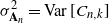 $\sigma_{\mathbf{A}_n}^2 = \operatorname{Var}[C_{n,k}]$
. By the symmetry of
 $\mathbf{A}_n$
, we have
 $x_{n,j,k} = x_{n, n-j+1,k}$
. With every
 $a_{i,j}$
being 0 or 1, and
 $a_{i.}=x_{n,i,k}/n$
,
 $a_{.j} = x_{n,n-j+1,k}/n$
, and the proportion of 1s in the matrix all being fractions, each of the four factors in Bolthausen’s bound is absolutely bounded by 1. We have the bound
 \begin{align*}\sup_{x}\biggl(\biggl|{\mathbb P}\biggl(\dfrac{C_{n,k_n} - {\mathbb E}[C_{n,k}]} {\sigma_{\mathbf{A}_n}} \le x\biggr) - \Phi(x)\biggr|\biggr)\le \dfrac K n \sum_{1\le i,j\le n} \biggl(\dfrac 4 {\sigma_{\mathbf{A}_n}}\biggr)^3 =\dfrac {64 K n}{\sigma_{\mathbf{A}_n}^3}. \end{align*}
The variance of
 $C_{n,k_n}$
in this regime is asymptotic to
 $\rho (\alpha)n$
(see Proposition 3.1). Asymptotic normality follows. After cleaning up via Slutsky’s theorem, we get
 \begin{align*}\dfrac {C_{n,k_n}- \alpha (2-\alpha) n} {\sqrt n} \ {\buildrel \mathcal{D} \over \longrightarrow}\ \mathcal{N}(0,\rho(\alpha)) \quad \text{as $ n \to\infty$;} \end{align*}
the rate of convergence is
 ${\mathrm{O}} (1/\sqrt n\,)$
. Recall that the linearity coefficient
 $\rho(\alpha)$
in the variance in the regime
 $(0,\tfrac{1}{2})$
is different from the linearity coefficient in the regime
 $[\tfrac{1}{2}, 1)$
(see the discussion in Section 3.1). For each part, we use the corresponding
 $\rho(\alpha)$
. Parts (c) and (d) are proved.
(e) Consider next the regime
 $k_n = n - g_n$
, for
 $g_n = {\mathrm{o}} (n)$
but growing faster than
 $\sqrt n$
. Again, we use Bolthausen’s theorem (Theorem 5.1). We examine the geometry of
 $\mathbf{A}_n$
. It has two corners filled with zeros. These are positions excluded from viewing. The top row has
 $g_n -1$
excluded cells flushed to its right end, the second row has
 $g_n-2$
excluded cells flushed to its right end, and so on until we reach row
 $g_n-1$
, which has one excluded cell at its rightmost position. There are
 $(g_n-1) + (g_n-2)+ \cdots +1 =g_n(g_n-1)/2 $
excluded cells in this top right corner. The lower left corner is a mirror image of the top right one. So we have exactly
 $(g_n-1)g_n$
excluded cells.
To the double sum (5.1) in Bolthausen’s theorem, a cell containing
 $a_{i,j}=1$
contributes
 \begin{align*}& \biggl|1 - \dfrac {x_{n,i,k}} n - \dfrac {x_{n,n-j+1,k}} n + \dfrac {n^2 -g_n(g_n-1)} {n^2}\biggr|^3 \\[3pt] &\quad = \biggl|1 - \dfrac {n-{\mathrm{O}} (g_n)} n - \dfrac {n-{\mathrm{O}} (g_n)} n + \dfrac {n^2 -g_n(g_n-1)} {n^2}\biggr|^3\\[3pt] & \quad = {\mathrm{O}}\biggl(\dfrac {g_n^3} {n^3}\biggr),\end{align*}
whereas a cell containing
 $a_{i,j}=0$
contributes
 \begin{align*} \biggl|0 - \biggl(1+ {\mathrm{O}}\biggl(\dfrac {g_n} n\biggr)\biggr) - \biggl(1+ {\mathrm{O}}\biggl(\dfrac {g_n} n\biggr)\biggr) + \biggl(1- {\mathrm{o}}\biggl(\dfrac {g_n} n\biggr)\biggr) \biggr|^3 = 1 + {\mathrm{O}}\biggl(\dfrac {g_n} n\biggr). \end{align*}
The double sum (5.1) in Bolthausen’s theorem amasses
 $(n^2 -g_n(g_n-1)){\mathrm{O}} ({{g_n^3}/{ }}{n^3})$
from the cells containing 1 and
 $g_n(g_{n-1})(1 + {\mathrm{O}} ({{g_n}/{ }}{n}))$
from the excluded zeros at the corners, a total double sum of order
 $g_n^2$
. The variance is asymptotic to
 $g_n^2/n$
and the overall bound is
 \begin{align*}\frac{{\mathrm{O}} \left(g_n^2\right) }{ n \Theta \left({{g_n^2 }/{ n}}\right)^{3/2}} = \Theta \biggl(\frac {\sqrt n} {g_n}\biggr). \end{align*}
The bound tends to 0 for the regime
 $k_n = n - g_n$
, with
 $n = {\mathrm{o}} (g_n^2)$
. Limiting Gaussianity follows. After cleaning up via Slutsky’s theorem, part (e) is proved.
(f) In the critical regime
 $k_n = n - g_n$
, with
 $g_n \sim c \sqrt n$
, and
 $c\in {\mathbb R}^+$
, we prove a Poisson limit. Let us first focus on
 $C_{n, k_n}' = n - C_{n,k_n}$
, which counts the number of permutation elements lying outside their viewing window.
The natural indexing by the set
 $\{1, \ldots, n\}$
gives bounds on the total variation distance that are too high to be of use. It is then helpful to work with refined indexing
 $\mathcal{I}$
, derived from the representation of
 $\{|\pi_i -i | > k_n\}$
as a union of individual atoms specified by locations on row i.
On row
 $i \in\{1, \ldots, g_n-1\}$
, the set
 $\mathcal{I}$
collects
 \begin{align*}\{(i,i+ k+1)\} \cup \{(i, i+k+2)\} \cup \cdots \cup \{(i,n)\}. \end{align*}
On row
 $i\in \{n-g_n+2, \ldots, n\}$
, the set
 $\mathcal{I}$
collects
 \begin{align*}\{(i,1)\} \cup \{(i,2)\} \cup \cdots \cup \{(i,i+g_n-n-1)\}. \end{align*}
On rows
 $i=g_n, \ldots, n-g_n +1$
, the sets
 $\{|\pi_i -i | > k_n\}$
are empty and add nothing to
 $\mathcal{I}$
. So the indexing set can be written as
 \begin{align*}\mathcal{I} = \Biggl(\bigcup_{i=1}^{g_n-1} \bigcup_{j=i+k+1}^n {\{(i,j)\}}\Biggr) \bigcup \Biggl(\bigcup_{i=n-g_n+2}^n \bigcup_{j=1}^{i+g_n-n-1} {\{(i,j)\}}\Biggr). \end{align*}
The size of the indexing set is
 $2((g_n-1)+(g_n -2) + \cdots +1) = g_n (g_n-1)$
.
For
 $(i,j)\in [n]\times [n]$
, define
 $X_{(i,j)}= \mathbf{1}_{\{\pi_i = j\}}$
. Now we have
 \begin{align*}C_{n,k_n}' = \sum_{i=1}^n \mathbf{1}_{\{|\pi_i -i | > k_n\}}= \sum_{i=1}^n \sum_{\alpha = (i,j)\in \mathcal{I}} X_{(i,j)}. \end{align*}
After all, with this representation,
 $C_{n,k_n}'$
is the sum of a large number of Bernoulli random variables, making the case a candidate for Poisson approximation via the Chen–Stein method.
In the Arratia–Goldstein–Gordon version of the Chen–Stein method (Theorem 5.2), take the dependency neighborhood corresponding to
 $\alpha=(i,j)\in\mathcal{I}$
to be
 \begin{align*}B_\alpha = \{\beta =(i', j') \colon i'=i {\ \rm or\ } j' = j\}. \end{align*}
In other words, we take
 $X_\beta$
to be in the dependency neighborhood of
 $X_\alpha$
if the cell specified by the pair
 $\beta= (i',j')$
in the matrix
 $\mathbf{A}_n$
is in the same row or column as
 $\alpha=(i,j)$
. The size of the dependency neighborhood of
 $\alpha \in \mathcal{I}$
is at most
 $g_n+ g_n-1 = 2g_n-1$
.
We next go through the calculation of the three components
 $b_1,b_2,b_3$
. For
 $b_1$
, we use that the size of
 $B_\alpha$
of any
 $\alpha\in \mathcal{I}$
is at most
 $2g_n-1$
, and the size of
 $\mathcal{I}$
is
 $g_n(g_n-1)$
, and that we are in the regime
 $g_n \sim c\sqrt n$
to get
 \begin{align*}b_1 =\sum_{\alpha \in \mathcal{I}}\dfrac {|B_\alpha|} {n^2} \le \dfrac {|\mathcal{I}| (2g_n-1)}{n^2} = \Theta\biggl(\dfrac 1 {\sqrt n}\biggr). \end{align*}
As no two elements can occupy the same location in the permutation, and no element appears in two places in the permutation, if
 $X_\alpha = 1$
, then
 $X_\beta=0$
for all
 $\beta\in B_\alpha- \{\alpha\}$
. Otherwise,
 $X_\alpha = 0$
. In both cases
 $X_\alpha X_\beta=0$
and
 $b_2=0$
.
The computation of
 $b_3$
requires conditioning on the variables
 $X_\beta$
, with
 $\beta$
in the subset
 $H_\alpha = \{\beta\in \mathcal{I}\colon \beta\not \in B_\alpha\}$
. By the geometry of the neighborhoods, if
 $X_\beta =1$
, for
 $\beta\in H_\alpha$
, then this deprives
 $X_\alpha$
from a position in the permutation, as
 $\beta \in H_\alpha$
specifies a cell in
 $\mathbf{A}_n$
in a different row and a different column from
 $\alpha$
. Therefore, for
 $\alpha = (i,j) \in \mathcal{I}$
, conditionally, there are
 $n - \sum_{\beta \in H_\alpha} X_\beta$
equally likely positions for i.
Observe that at most one among the Bernoulli random variables in a row within
 $\mathcal{I}$
can equal 1 (an element of [n] cannot be at two positions in the permutation). In other words, the sum of all the Bernoulli random variables on the same row of
 $\mathcal{I}$
is one combined Bernoulli random variable. Conditionally, there are
 \begin{align*}n - \sum_{\substack{i'=1 \\[3pt] i'\not =i}}^{g_n-1} \tilde X_{i'} - \sum_{\substack{i''=n-g_n+2 \\[3pt] i''\not =i}}^n \tilde X_{i''} , \end{align*}
for Bernoulli random variables
 \begin{align*}\tilde X_{i'} = \sum_{j=n-g_n+i'+1}^n X_{(i',j)} \quad \text{for $ i' \in\{ 1 ,\ldots, g_n-1\}$,} \end{align*}
and
 \begin{align*}\tilde X_{i''} = \sum_{j=1}^{i''-n+g_n-1} X_{(i'',j)} \quad \text{for $ i'' \in \{ n-g_n+2 ,\ldots, n\}$.} \end{align*}
So we have
 \begin{align*} b_3 &= \sum_{\alpha =(i,j)\in \mathcal{I}} \mathbb{E}\left[\dfrac{1}{n - \sum_{\substack{i'=1 \\ i'\neq i}}^{g_n-1} \tilde{X}_{i'} - \sum_{\substack{i''=n-g_n+2 \\ i''\neq i}}^n \tilde{X}_{i''}} - \dfrac{1}{n}\right] \\[3pt] &= \sum_{\alpha \in \mathcal{I}} \mathbb{E}\left[\dfrac{\sum_{\substack{i'=1 \\ i'\neq i}}^{g_n-1}\tilde{X}_{i'} + \sum_{\substack{i''=n-g_n+2 \\ i''\neq i}}^n \tilde{X}_{i''}}{n\Big(n - \sum_{\substack{i'=1 \\ i'\neq i}}^{g_n-1}\tilde{X}_{i'} - \sum_{\substack{i''=n-g_n+2 \\[3pt] i''\neq i}}^n \tilde{X}_{i''}\Big)}\right] \end{align*}
 \begin{align*} &\le \sum_{\alpha \in \mathcal{I}} \dfrac{2(g_n-1)}{n(n - 2 (g_n-1))} \\[3pt] &= \dfrac{2|\mathcal{I}|\, (g_n-1)}{n(n - 2(g_n-1))} \\[3pt] &= \dfrac{\mathrm{O}(g^3(n))}{\Theta(n^2)} \\[3pt]&= \mathrm{O}\left(\dfrac{1}{\sqrt{n}}\right). \end{align*}
With
 $b_2=0$
and both
 $b_1$
and
 $b_3$
being of order
 $1/ \sqrt n$
, in Theorem 5.2, we get to the conclusion that
 \begin{align*}d_{\textit{TV}} \bigl(C_{n,k_n}', \operatorname{Poi}\bigl({\mathbb E}\bigl[C_{n,k_n}'\bigr]\bigr)\bigr) = {\mathrm{O}}\biggl(\dfrac 1 {\sqrt n}\biggr). \end{align*}
By the triangle inequality, we have
 \begin{align*}d_{\textit{TV}} \bigl(C_{n,k_n}', \operatorname{Poi}(c^2)\bigr) &\le d_{\textit{TV}} \bigl(C_{n,k_n}',\operatorname{Poi}\bigl({\mathbb E}\bigl[C_{n,k_n}'\bigr]\bigr)\bigr) + d_{\textit{TV}} \bigl(\operatorname{Poi}\bigl({\mathbb E}\bigl[C_{n,k_n}'\bigr], \operatorname{Poi}(c^2)\bigr)\bigr)\\[3pt] &= {\mathrm{O}}\biggl(\dfrac 1 {\sqrt n}\biggr) + d_{\textit{TV}} \bigl(\operatorname{Poi}\bigl({\mathbb E}\bigl[C_{n,k_n}'\bigr], \operatorname{Poi}(c^2)\bigr).\end{align*}
As shown in [Reference Lyon and Mahmoud12, Lemma 4.2], the total variation distance between two Poisson distributions is at most the absolute difference between their parameters. So we have
 \begin{align*} d_{\textit{TV}} \bigl(\operatorname{Poi}\bigl({\mathbb E}\bigl[C_{n,k_n}'\bigr], \operatorname{Poi}(c^2)\bigr)\bigr) = \bigl|n -{\mathbb E}\bigl[C_{n,k_n}\bigr] - c^2\bigr|. \end{align*}
The expectation of
 $C_{n,k_n}$
is given in Proposition 2.1. After a calculation, we find that the latter total variation distance is
 ${\mathrm{O}} (1/ \sqrt n\,)$
too. We have arrived at
 \begin{align*}d_{\textit{TV}} \bigl(n - C_{n,k_n}, \operatorname{Poi}(c^2)\bigr) \to 0 \quad \text{as $ n \to \infty$,} \end{align*}
which implies that
 $n - C_{n,k_n}\, {\buildrel \mathcal{D} \over \longrightarrow}\, \operatorname{Poi}(c^2)$
. Part (f) is proved.
(g) In the extremal regime
 $n-g_n$
, with
 $g_n = {\mathrm{o}} (\sqrt n\,)$
, the variance is
 ${\mathrm{O}} (g_n^2/n)$
. For every
 $\varepsilon >0$
, the Chebyshev inequality gives
 \begin{align*}{\mathbb P} \bigl(\bigl|C_{n, k_n} - {\mathbb E}\bigl[C_{n, k_n}\bigr] \bigr|> \varepsilon\bigr) \le \dfrac{{\mathrm{O}} \left(g_n^2/n\right)} {\varepsilon^2} \to 0 \quad \text{as $ n \to\infty$,} \end{align*}
which means
 $C_{n, k_n} - {\mathbb E}[C_{n, k_n}]\buildrel {\mathbb P} \over \longrightarrow 0$
. It is discussed in Section 2.1 that
 $ {\mathbb E}[C_{n, k_n}] -n \to 0.$
The addition rule of probabilistic convergence relations proves part (g).
6. A retrospective look at the phases
For the purpose of convergence, we kept k fixed in Theorem 5.3(a). In the case of k growing, the bounds in (5.3) remain valid, but it is crucial to keep
 $k_n$
in the low
 ${\mathrm{o}} (n)$
regime. The reason is that for the argument of the lower bound, for any fixed r, however large, we need to be able to pack r non-intersecting windows of width
 $2k_n+1$
over n positions to construct
 $Q_{n,k_n}'$
. This requires
 $r (2k_n+1) \le n$
. For r arbitrarily large, we need
 $r \le n/(2k_n+1)$
for
 $n \to\infty$
. Thus
 $n/k_n$
must diverge to infinity. Without the stipulation that
 $k_n = {\mathrm{o}} (n)$
, the argument breaks down for not keeping the lower bound of the same order as the upper bound.
A case in point is
 $k_n =n-1$
, for which the product of the indicators is a Bernoulli random variable with success probability 1 (every element is seen within its associated window,
 $C_{n,n-1}=n$
) and the rth factorial moment of
 $C_{n,n-1}$
is
 $(n)_r$
, for
 $r\ge 2$
, not bounded below by
 $(2(n-1)+1)^r$
.
For
 $k_n = {\mathrm{o}} (n)$
, we can approximate the distribution of the
 $k_n$
-window statistic by that of
 $\operatorname{Poi}(2k_n+1)$
, which in turn is normal in view of the size of its parameter, as in part (b) of Theorem 5.3, for example.
Chen–Stein Poisson approximation could be used to prove part (a). It is also possible to use the method in the regime
 $k_n = n -g_n$
, with
 $g_n ={\mathrm{o}} (\sqrt n\,)$
. However, in this case we get convergence of
 $C_{n,k_n}-n$
to
 $\operatorname{Poi}(0)$
, which would look a bit artificial. In any case, such convergence to
 $\operatorname{Poi}(0)$
is identical to the result in part (g).
In the Arratia–Goldstein–Gordon version [Reference Arratia, Goldstein and Gordon1] of the Chen–Stein method, the authors speak of dependency neighborhood sets
 $B_\alpha$
of
 $X_\alpha$
, outside which the variables
 $X_\beta$
, for
 $\beta\not \in B_\alpha$
, are independent or ‘nearly independent’ of
 $X_\alpha$
. In practice, such neighborhoods are not unique. The author ultimately selected
 $B_\alpha$
as in the proof of Theorem 5.3(f) to keep the argument in the spirit of Example 1.3 in [Reference Arratia, Goldstein and Gordon2] and create a context for comparison.
Remark 6.1. The distribution of the 0-window statistic (the number of fixed points) has long been known to be
 $\operatorname{Poi}(1)$
(see [Reference Barbour, Holst and Janson4, Example 3.4.2]). This agrees with the statement of Theorem 5.3(a), when
 $k=0$
.
Remark 6.2. The convergence in part (f) to
 $\operatorname{Poi}(c^2)$
is consistent with the computations of the mean and variance in Sections 2.1 and 3.1: the Poison distribution
 $\operatorname{Poi}(c^2)$
has mean
 $c^2$
and variance
 $c^2$
, conforming to
 $\lim_{n\to \infty} {\mathbb E}[C_{n,k}] = c^2$
(from Proposition 2.1) and
 $\lim_{n\to \infty}$
 $\operatorname{Var}[C_{n,k}] = c^2$
(from Proposition 3.1).
7. A note on the use of AI
The author attempted to use AI and it was a very mixed experience, often frustrating, but there were also bright moments with happy endings. AI cannot construct mathematical logic and often makes gross mistakes. Nevertheless, on occasion it suggested references and useful directions, even though it could not execute them well.
The specific AI consulted is ChatGPT-5.2. One example of where AI was misleading is as follows. The author asked for references on the Poisson limit for fixed points. ChatGPT claimed it is in Feller’s book [Reference Feller7], specifying Section 6.2. Upon checking Section 6.2, one cannot find a discussion of fixed points in permutations; rather, one finds a discussion of derangements, which count something different. The author went back and pressed ChatGPT for better answers. The chat became defensive and evasive, claiming that there are multiple editions of the book and possibly the discussion is in the Indian edition. This was a waste of time with no good outcome.
As an example of lack of technical ability, the author consulted ChatGPT on the dependency neighborhoods in the Chen–Stein method. The author did not have extensive experience with the Chen–Stein method when applied to dependent random variables. The announcement in [Reference Arratia, Goldstein and Gordon2] that the complement of the dependency neighborhoods includes independent or ‘nearly independent’ random variables left the author baffled. He then asked ChatGPT for clarification. The answer was reasonable: these neighborhoods are not unique. The author then chose the one in the proof of Theorem 5.3(f) which works. He then wondered if a simpler neighborhood like just the set
 $\{\alpha\}$
might work. ChatGPT concurred that it is a ‘risky’ dependency neighborhood. The author then asked ChatGPT to go through the calculation with this reduced neighborhood. It came back concluding that it does not work. After hand checking, the author found that indeed
 $b_1, b_2$
, and
 $b_3$
converge to 0. Chen–Stein Poisson approximation goes through with this choice; the chat’s answer is false. This gross error was reported to ChatGPT. It acknowledged its mistake and apologized ☺.
However, ChatGPT was helpful in resolving multiple technical writing issues that would otherwise consume an enormous amount of time to investigate and find the right sources. As an example, the author impressed on the AI that the scientific community prefers for citations to books and long papers to specify a location, such as a range of pages or a section. ChatGPT concurs that this is a better style. It was then asked how to produce such a citation. ChatGPT gave a useful tip on this, providing the LaTeX code
 \begin{align*}\backslash \text{cite[Example 3.4.2]\{Holst\}} \end{align*}
for the citation [Reference Barbour, Holst and Janson4, Example 3.4.2] used in Section 1.
The author is sharing this information in the hope that it will help other researchers, particularly junior researchers, understand the scope, limitations, pitfalls, and areas of strength of AI. It is also hoped that it will help AI developers improve their designs.
Appendix
We expand the four-fold sums in
 $L_{n,k}$
to write it in the form
 \begin{align*}L_{n,k} &= \sum_{1\le i,j\le n} \sum_{r=1}^n \mathbf{J}_{r,i,k} \sum_{\substack{s=1\\[3pt] s\not = r}}^n \mathbf{J}_{s,j,k}\\[3pt] &= \sum_{1\le i,j\le n} \sum_{r=1}^n \mathbf{J}_{r,i,k} \Biggl(\Biggl(\sum_{s=1}^n \mathbf{J}_{s,j,k}\Biggr) - \mathbf{J}_{r,j,k}\Biggr)\\[3pt] &= \sum_{1\le i,j\le n} \Biggl(\sum_{r=1}^n \mathbf{J}_{r,i,k}\Biggr) \Biggl(\sum_{s=1}^n \mathbf{J}_{s,j,k}\Biggr) - \sum_{1\le i,j\le n} \sum_{r=1}^n \mathbf{J}_{r,i,k}\, \mathbf{J}_{r,j,k}\\[3pt] &= \sum_{1\le i,j\le n} \Biggl(\sum_{r=1}^n \mathbf{J}_{r,i,k}\Biggr) \Biggl(\sum_{s=1}^n \mathbf{J}_{s,j,k}\Biggr) - \sum_{1\le i,j\le n} \sum_{r=1}^n \mathbf{J}_{i,r,k}\, \mathbf{J}_{j,r,k} \quad (\mathbf{A}_n \ \text{is symmetric})\\[3pt] &= \sum_{1\le i,j\le n} \Biggl(\sum_{r=1}^n \mathbf{J}_{r,i,k}\Biggr) \Biggl(\sum_{s=1}^n \mathbf{J}_{s,j,k}\Biggr) - \sum_{r=1}^ n \sum_{i=1}^n \mathbf{J}_{i,r,k}\sum_{j=1}^n \mathbf{J}_{j,r,k}.\end{align*}
Similarly, we have
 \begin{align*}M_{n,k} &= \sum_{i=1}^n \sum_{r=1}^n \mathbf{J}_{r,i,k} \sum_{\substack{s=1\\ s\not = r}}^n \mathbf{J}_{s,i,k} \end{align*}
 \begin{align*} &= \sum_{i=1}^n \sum_{r=1}^n \mathbf{J}_{r,i,k} \Biggl(\Biggl(\sum_{s=1}^n \mathbf{J}_{s,i,k}\Biggr) - \mathbf{J}_{r,i,k}\Biggr)\\[3pt] &= \sum_{i=1}^n \Biggl(\sum_{r=1}^n \mathbf{J}_{r,i,k}\Biggr) \Biggl(\sum_{s=1}^n \mathbf{J}_{s,i,k}\Biggr) - \sum_{i=1}^n \sum_{r=1}^n \mathbf{J}_{r,i,k}.\end{align*}
Again, the sum
 $x_{n,i,k} =\sum_{r=1}^n\mathbf{J}_{r,i,k}$
is key to these calculations. In the proof of Proposition 2.1, we have worked out the structure of
 $x_{n,i,k}$
in both the lower regime
 $0\le k< n/2$
and the upper regime
 $n/2 \le k$
. In these terms, we write
 \begin{equation}L_{n,k} = \Biggl(\sum_{i=1}^n x_{n,i,k}\Biggr)^2 - \sum_{i=1}^nx_{n,i,k}^2\end{equation}
and
 \begin{equation}M_{n,k} = \sum_{i=1}^n x_{n,i,k}^2 - \sum_{i=1}^nx_{n,i,k}.\end{equation}
The sum
 $\sum_{i=1}^nx_{n,i,k}$
is evaluated in (2.1) and the formula for the regime
 $0 \le k < n/2$
is the same as for the regime
 $ n/2 \le k \le n-2$
. Unlike this situation, the sum
 $\sum_{i=1}^nx_{n,i,k}^2$
is different in the two regimes, and we have to consider the two cases separately.
The regime
 $k< n/2$
. In this regime we have
 \begin{align}\sum_{i=1}^n x_{n,i,k}^2 &= \sum_{i=1}^k (k+i)^2 + \sum_{i=k+1}^{n-k} (2k+1)^2 + \sum_{i=n-k+1}^ n (k+1+n-i)^2\nonumber \\[3pt] &=(2k+1)\biggl((2k+1) n - \dfrac 5 3 k(k+1)\biggr). \end{align}
We plug (2.1) and (A.3) into (A.1) to find
 \begin{align*}L_{n,k} =(2k+1)((2k+1) n^2 - (2k^2 + 4k +1)n) + \dfrac 1 3 k(k+1)(3k^2+13k +5). \end{align*}
We finish the computation by substituting (2.1) and (A.3) in (A.2), which gives
 \begin{align*}M_{n,k} = 2k(2k+1)n -\dfrac 2 3 k (k + 1)(5k + 1). \end{align*}
The regime
 $k \ge n/2$
. The sum
 $\sum_{i=1}^n x_{n,i,k}$
is the same expression as the counterpart in the case
 $k < n/2$
.
Again,
 $\sum_{i=1}^n x_{n,i,k}^2$
does not come out the same as its counterpart in the case
 $k< n/2$
. Here we have
 \begin{align}\sum_{i=1}^n x_{n,i,k}^2 &= \sum_{i=1}^{n-k-1} (k+i)^2 + \sum_{i=n-k}^{k+1} n^2 + \sum_{i=k+2}^n (k+n+1-i)^2\nonumber \\[3pt] &=\dfrac 1 3 (- n^3 +3 (2k+1)n^2 + n - k (k+1) (2 k + 1)). \end{align}
Using (2.1) and (A.4) in (A.1), we get
 \begin{align*}L_{n,k} = \dfrac 1 3 n^3 + 2k(2k+1)n^2 - \biggl( 4k^3 +6k^2 +2k + \dfrac 1 3\biggr) n+ \dfrac 1 3 k(k+1) (3k^2 +5k +1). \end{align*}
We finish the computation by substituting (2.1) and (A.4) in (A.2), which gives
 \begin{align*}M_{n,k} = -\dfrac {n^3} 3 + (2k + 1)n^2 - \biggl(2k + \dfrac 2 3\biggr)n -\dfrac {2k} 3(k^2-1). \end{align*}
Acknowledgements
The author is indebted to Svante Janson for encouragement and sound advice directing him to lines of attack that proved quite effective in this research. The careful critique by two anonymous referees improved the exposition and rid it of some small errors.
This work was completed while the author was on sabbatical leave at The Catholic University of America in Fall 2025. He thanks the Department of Mathematics and Statistics there for their gracious reception and hospitality, and for an environment conducive to research under the leadership of Kiran Bhutani.
Funding information
There are no funding bodies to thank relating to the creation of this article.
Competing interests
There were no competing interests to declare which arose during the preparation or publication process of this article.
 Π8=(3,8,1,6,2,7,5,4)
 8×8
 (i,πi)
 |i−j|≤k
 k=2
 k=5
 kn
 ρ(α)
 α


