I enjoyed reading the target article by Bruineberg et al. and fully endorse the authors' agenda of ambiguity resolution. In this spirit, it is worth beginning this article by carefully considering what we mean by the words we choose, and specifically by the word “model.” The definition of a model is a subject that deserves much more space than is available for this commentary. However, the use of the term by the authors of the target article suggests a very simple definition of the sort of model we are interested in. For the purposes of this commentary, a model is another word for a joint probability distribution. The graphical models of the target article can be derived simply from this starting point (Wainwright & Jordan, Reference Wainwright and Jordan2008).
Under this definition of a model, it follows that a Markov blanket, itself defined in terms of conditional probabilities (Pearl, Reference Pearl1988), must always be defined in relation to a model. This raises the question of where models come from. One source of the probability distributions that make up a model is the potential function, Hamiltonian, or steady-state density of some dynamical system (Friston & Ao, Reference Friston and Ao2012). This represents a model of a specific sort of (time-evolving) system. Bruineberg et al. suggest that this means blankets in such systems are different in nature to those in other kinds of systems. However, the identification of a Markov blanket in such a model is no different to its identification in any other model.
As such, the key distinction is not between different kinds of Markov blankets. A taxonomy of models, from which conditional independencies can be identified, may be a more meaningful way of addressing the implicit distinctions. Bruineberg et al. make some steps towards this, subcategorising models in several different ways. For instance, they highlight the distinction between our model of some system versus some (sentient) system's model of its world (Friston, Wiese, & Hobson, Reference Friston, Wiese and Hobson2020). While many of these were interesting, the distinction that I found most intriguing was that between a model in which the Markov blanket plays the role of a “physical” boundary and one in which it offers only a “statistical” boundary.
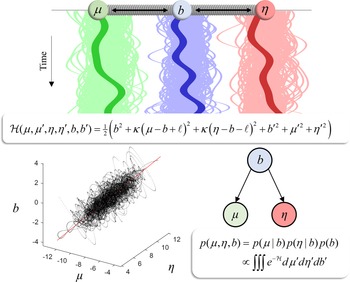
So, what is it that makes a boundary physical? The remainder of this commentary explores this question, assuming that physical is here synonymous with spatial, with the aid of an example system depicted in Figure 1. Here, we have three beads on a string, separated by springs. If two beads become too close, the compressed spring pushes them away from one another. If too far apart, the extended spring pulls them back together.
Figure 1.Spatial boundaries. This figure depicts an example system that can be interpreted as having a “physical” boundary. It comprises three beads (with positions μ, η, and b, and velocities indicated by prime notation) separated by two springs with equilibrium lengths ℓ. The Hamiltonian (ℋ) incorporates the potential energies associated with the springs, and the kinetic energies of each bead. The decomposition of the Hamiltonian into a sum of terms ensures the associated steady-state density is consistent with the conditional independencies required for a Markov blanket. Interpreting this steady state as a model, we can express it as a Bayesian network (lower right). The trajectories of each bead are shown at the top of the figure, showing many trajectories with different initial conditions (sampled from the steady-state density). An example trajectory is superimposed upon each. The lower left plot shows all simulated trajectories plotted in three dimensions, with the direction of the first principal component shown in red.
In this example, the positions of each bead collectively constitute a three-dimensional system (as plotted in the lower left). What is it that licenses us to embed each of these along a single spatial dimension, such that it is meaningful to describe the positions of objects relative to one another? Only by doing so can we talk of spatial boundaries for which it would be surprising to observe one element of the system cross from one side of this boundary to the other.
The steady-state density implicit in this system's Hamiltonian factorises to reveal a Markov blanket. Specifically, the positions of the left and right beads are conditionally independent of one another given the central bead. This means the middle bead's position is a Markov blanket for the positions of the other two beads. Another way of putting this is that all covariance shared between the left and right beads is dependent upon the middle bead. The lower left plot of Figure 1 illustrates this heuristically by plotting multiple trajectories with different initialisations to give a sense of the shape of the joint probability density. Note that the axis that accounts for most of the variance (shown in red) is a linear combination of the original three axes.
The use of prepositions (left, right, and middle) in describing the beads is crucial in interpreting the Markov blanket implied by this model as a spatial boundary. Clearly it would be meaningless to plot the three positions on the same axis (as in the upper plot of Fig. 1) if their positions relative to one another played no role in their behaviour. The model of the beads ensures pairs of adjacent beads constrain one another's positions such that (for example) it would be very surprising to find two beads in the same spatial location.
In short, a model that lends itself towards an interpretation of its Markov blankets as spatial boundaries must exhibit the following features:
(1) The probability density associated with the model must have a non-spherical covariance structure. This is guaranteed by the presence of a non-trivial Markov blanket.
(2) The pair of conditional densities describing the positions of the variables partitioned by the blanket, given the blanket, must assign very low probability to positions immediately proximate to the position of the blanket. This is achieved in our example via the repulsive forces when the springs were compressed.
(3) The model must be interpretable as a steady-state density. This implies a system that evolves in time but whose density dynamics, when initialised at the steady state, are static. The time evolution is important in that it provides an explicit link between the model and the Lagrangians and Hamiltonians found in physics.
Presumably, one of the reasons Bruineberg et al. highlighted the special case in which Markov blankets take on the flavour of spatial boundaries is that they are sometimes called upon (Ramstead, Badcock, & Friston, Reference Ramstead, Badcock and Friston2018) in an attempt to address Schrödinger's famous question about the physics of life (Schrödinger, Reference Schrödinger1944), formulated explicitly in terms of a spatial boundary. This commentary was written to question whether such boundaries require special kinds of Markov blankets and suggests that, instead, they require special kinds of model.






 You have
Access
I enjoyed reading the target article by Bruineberg et al. and fully endorse the authors' agenda of ambiguity resolution. In this spirit, it is worth beginning this article by carefully considering what we mean by the words we choose, and specifically by the word “model.” The definition of a model is a subject that deserves much more space than is available for this commentary. However, the use of the term by the authors of the target article suggests a very simple definition of the sort of model we are interested in. For the purposes of this commentary, a model is another word for a joint probability distribution. The graphical models of the target article can be derived simply from this starting point (Wainwright & Jordan, Reference Wainwright and Jordan2008).
Under this definition of a model, it follows that a Markov blanket, itself defined in terms of conditional probabilities (Pearl, Reference Pearl1988), must always be defined in relation to a model. This raises the question of where models come from. One source of the probability distributions that make up a model is the potential function, Hamiltonian, or steady-state density of some dynamical system (Friston & Ao, Reference Friston and Ao2012). This represents a model of a specific sort of (time-evolving) system. Bruineberg et al. suggest that this means blankets in such systems are different in nature to those in other kinds of systems. However, the identification of a Markov blanket in such a model is no different to its identification in any other model.
As such, the key distinction is not between different kinds of Markov blankets. A taxonomy of models, from which conditional independencies can be identified, may be a more meaningful way of addressing the implicit distinctions. Bruineberg et al. make some steps towards this, subcategorising models in several different ways. For instance, they highlight the distinction between our model of some system versus some (sentient) system's model of its world (Friston, Wiese, & Hobson, Reference Friston, Wiese and Hobson2020). While many of these were interesting, the distinction that I found most intriguing was that between a model in which the Markov blanket plays the role of a “physical” boundary and one in which it offers only a “statistical” boundary.
So, what is it that makes a boundary physical? The remainder of this commentary explores this question, assuming that physical is here synonymous with spatial, with the aid of an example system depicted in Figure 1. Here, we have three beads on a string, separated by springs. If two beads become too close, the compressed spring pushes them away from one another. If too far apart, the extended spring pulls them back together.
Spatial boundaries. This figure depicts an example system that can be interpreted as having a “physical” boundary. It comprises three beads (with positions μ, η, and b, and velocities indicated by prime notation) separated by two springs with equilibrium lengths ℓ. The Hamiltonian (ℋ) incorporates the potential energies associated with the springs, and the kinetic energies of each bead. The decomposition of the Hamiltonian into a sum of terms ensures the associated steady-state density is consistent with the conditional independencies required for a Markov blanket. Interpreting this steady state as a model, we can express it as a Bayesian network (lower right). The trajectories of each bead are shown at the top of the figure, showing many trajectories with different initial conditions (sampled from the steady-state density). An example trajectory is superimposed upon each. The lower left plot shows all simulated trajectories plotted in three dimensions, with the direction of the first principal component shown in red.
In this example, the positions of each bead collectively constitute a three-dimensional system (as plotted in the lower left). What is it that licenses us to embed each of these along a single spatial dimension, such that it is meaningful to describe the positions of objects relative to one another? Only by doing so can we talk of spatial boundaries for which it would be surprising to observe one element of the system cross from one side of this boundary to the other.
The steady-state density implicit in this system's Hamiltonian factorises to reveal a Markov blanket. Specifically, the positions of the left and right beads are conditionally independent of one another given the central bead. This means the middle bead's position is a Markov blanket for the positions of the other two beads. Another way of putting this is that all covariance shared between the left and right beads is dependent upon the middle bead. The lower left plot of Figure 1 illustrates this heuristically by plotting multiple trajectories with different initialisations to give a sense of the shape of the joint probability density. Note that the axis that accounts for most of the variance (shown in red) is a linear combination of the original three axes.
The use of prepositions (left, right, and middle) in describing the beads is crucial in interpreting the Markov blanket implied by this model as a spatial boundary. Clearly it would be meaningless to plot the three positions on the same axis (as in the upper plot of Fig. 1) if their positions relative to one another played no role in their behaviour. The model of the beads ensures pairs of adjacent beads constrain one another's positions such that (for example) it would be very surprising to find two beads in the same spatial location.
In short, a model that lends itself towards an interpretation of its Markov blankets as spatial boundaries must exhibit the following features:
(1) The probability density associated with the model must have a non-spherical covariance structure. This is guaranteed by the presence of a non-trivial Markov blanket.
(2) The pair of conditional densities describing the positions of the variables partitioned by the blanket, given the blanket, must assign very low probability to positions immediately proximate to the position of the blanket. This is achieved in our example via the repulsive forces when the springs were compressed.
(3) The model must be interpretable as a steady-state density. This implies a system that evolves in time but whose density dynamics, when initialised at the steady state, are static. The time evolution is important in that it provides an explicit link between the model and the Lagrangians and Hamiltonians found in physics.
Presumably, one of the reasons Bruineberg et al. highlighted the special case in which Markov blankets take on the flavour of spatial boundaries is that they are sometimes called upon (Ramstead, Badcock, & Friston, Reference Ramstead, Badcock and Friston2018) in an attempt to address Schrödinger's famous question about the physics of life (Schrödinger, Reference Schrödinger1944), formulated explicitly in terms of a spatial boundary. This commentary was written to question whether such boundaries require special kinds of Markov blankets and suggests that, instead, they require special kinds of model.
Financial support
The Wellcome Centre for Human Neuroimaging is supported by core funding (203147/Z/16/Z).
Conflict of interest
None.