





1. Introduction
Let us start with the classical branching process without immigration. Analyzing the tail asymptotics of the density of the martingale limit of supercritical Galton–Watson processes began in [Reference Harris9]. We will discuss the Schröder case, where the minimum family size is exactly one. For a small argument of the density, analysis of the first asymptotic term began in [Reference Dubuc7], where precise estimates were obtained. Then, in [Reference Biggings and Bingham2], the authors found an explicit form of the first asymptotic term. After that, in [Reference Kutsenko13], the complete left-tail asymptotic was derived. All the asymptotic terms were expressed explicitly through the so-called one-periodic Karlin–McGregor function introduced in [Reference Karlin and McGregor10, Reference Karlin and McGregor11]. Moreover, it was shown that the series converges everywhere, not only for small arguments of the density. For the Galton–Watson processes with immigration, results are available only for the first asymptotic terms; see, e.g., [Reference Berestycki, Gantert, Mörters and Sidorova1, Reference Chu, Li and Ren3]. We will extend the results from [Reference Kutsenko13] to the case with immigration. It is impossible to directly apply the results of [Reference Kutsenko13] to this case, and we need to develop new techniques.
The Galton–Watson process with immigration is defined by
 \begin{equation*} X_{\mathrm{imm},t+1}=\sum_{j=1}^{X_{\mathrm{imm},t}}\xi_{j,t}+Y_t, \quad X_{{\rm imm},0}=1, \quad t\in{\mathbb N}\cup\{0\},\end{equation*}
where all the
 $\xi_{j,t}$
are independent and identically distributed natural-number-valued random variables with the probability-generating function
 $P(z)\,:\!=\,\mathbb{E}z^{\xi}=p_1z+p_2z^2+p_3z^3+\cdots$
. We consider the so-called Schröder case,
 $p_0=0$
and
 $0<p_1<1$
. For simplicity, we assume that P(z) is analytic in a neighborhood of
 $z=1$
– in particular, the offspring mean
 $\mu=P'(1)$
is finite. In terms of random variables
 $\xi_{j,t}$
, this means that their tails are light enough that the exponential moments are finite.
All immigration terms
 $Y_t$
are also identically distributed and independent of other terms. Their probability-generating function is
 $Q(z)\,:\!=\,\mathbb{E}z^{Y}=q_0+q_1z+q_2z^2+\cdots$
. We assume that
 $q_0\ne 0$
– sometimes, immigrants may not arrive. The assumption
 $p_1q_0 > 0$
is a complete analog of the Schröder case
 $p_1 > 0$
in the case without immigration, since these assumptions are equivalent to
 $\mathbb{P}(X_t = X_{t+1}) > 0$
.
For simplicity, we may require that Q(z) is entire; then we can define (19) and (23), and write (25), without trouble. The easiest relaxation is that Q(z) is analytic in a neighborhood of 1 and on the zero component of the filled Julia set
 $\mathscr{J}_P^{\kern1pt 0}$
, see the definition below. Often the zero component is bounded,
 $\mathscr{J}_P^{\kern1pt 0}\subset\{z\colon |z|\leqslant R\}$
with
 $R>1$
, and both conditions can be replaced by a stronger, but simpler, one: the series representing Q(z) converges at
 $z=R$
. Further relaxations can be achieved by imposing deeper harmonization requirements on P(z) and Q(z), but this will complicate the presentation.
The difference from the classical Galton–Watson process is the presence of new arrivals at each time step. Thus, instead of the classical probability-generating function of the Galton–Watson process
 $ X_t$
without immigration (
 $Q\equiv1$
),
 \begin{equation} P_{t}(z)=\underbrace{P\circ\cdots\circ P}_{t}(z)=\sum_{n=1}^{+\infty}\mathbb{P}( X_{t}=n)z^n,\end{equation}
satisfying
 $P_{t}(z)=P_{t-1}(P(z))$
and
 $P_0(z)\,:\!=\,z$
, we have
 \begin{equation} P_{\mathrm{imm},t}(z)=P_{\mathrm{imm},t-1}(P(z))Q(z)=\sum_{n=1}^{+\infty}\mathbb{P}(X_{\mathrm{imm},t}=n)z^n\end{equation}
in the case of immigration, which is
 \begin{equation} P_{\mathrm{imm},t}(z)=\underbrace{P\circ\cdots\circ P}_{t}(z)\cdot Q(\underbrace{P\circ\cdots\circ P}_{t-1}(z))\cdots Q(P(z))\cdot Q(z), \qquad P_{\mathrm{imm},0}(z)\,:\!=\,z.\end{equation}
To formulate the main result, we extract some information from [Reference Kutsenko13] and the next section. For the classical case
 $Q\equiv1$
, the density p(x) of the martingale limit
 $W=\mu^{-t}X_t$
can be computed as a Fourier transform of some special function:
 \begin{equation} p(x)=\frac1{2\pi}\int_{-\infty}^{+\infty}\Pi(\mathrm{i}y){\mathrm{e}}^{\mathrm{i}yx}\,{\mathrm{d}}y,\end{equation}
where
 $\Pi(z)$
is given by
 \begin{equation} \Pi(z)\,:\!=\,\lim_{t\to+\infty}\underbrace{P\circ\cdots\circ P}_{t}(1-{\mu^{-t}}z),\end{equation}
and it satisfies a Poincaré-type functional equation
 \begin{equation} P(\Pi(z))=\Pi(\mu z), \qquad \Pi(0)=1, \qquad \Pi'(0)=-1.\end{equation}
The Fourier inversion formula (4) for the density is well known – see, e.g., [Reference Dubuc7, Reference Fleischmann and Wachtel8]. The functional equation (6) is fundamental in the analysis of p(x). Defining another analytic function,
 \begin{equation} \Phi(z)\,:\!=\,\lim_{t\to+\infty}p_1^{-t}P_t(z),\end{equation}
satisfying the Schröder-type functional equation
 $\Phi(P(z))=p_1\Phi(z)$
,
 $\Phi(z)\sim z$
for
 $z\to0$
, we can use the one-periodic Karlin–McGregor function
 \begin{equation} K(z)\,:\!=\,p_1^{-z}\Phi(\Pi(\mu^z))\end{equation}
to obtain the complete left-tail series for p(x), which converges pointwise everywhere, not only for small
 $x>0$
. This research was done in [Reference Kutsenko13]. The Karlin–McGregor functions are discussed in detail in [Reference Karlin and McGregor10, Reference Karlin and McGregor11].
For the Galton–Watson process with immigration, by analogy with (4) (see also some details in [Reference Sidorova16]), the density
 $p_\mathrm{imm}(x)$
of the martingale limit
 $W_\mathrm{imm}=\lim_{t\to+\infty}\mu^{-t}X_{\mathrm{imm},t}$
can be computed as a Fourier transform of another special function,
 \begin{equation} p_\mathrm{imm}(x)=\frac1{2\pi}\int_{-\infty}^{+\infty}\Pi_\mathrm{imm}(\mathrm{i}y){\mathrm{e}}^{\mathrm{i}yx}\,{\mathrm{d}}y,\end{equation}
where, see (5) and (3),
 $\Pi_\mathrm{imm}(z)=\lim_{t\to+\infty}P_{\mathrm{imm},t}(1-{\mu^{-t}}z)=\Pi(z)\cdot R(z)$
, with
 $$R(z)=\prod_{t=1}^{+\infty}Q(\Pi({\mu^{-t}}z))$$
satisfying the functional equation
 $R(\mu z)=R(z)Q(\Pi(z))$
,
 $R(0)=1$
. There are no more Poincaré-type functional equations. However, we may still define a one-periodic function
 $L(z)\,:\!=\,q_0^{-z}{R(\mu^z)}{\Psi(\Pi(\mu^z))}$
with the help of another analytic function,
 $$\Psi(z)\,:\!=\,\prod_{t=0}^{+\infty}q_0^{-1}Q(\underbrace{P\circ\cdots\circ P}_{t}(z)),$$
satisfying another functional equation,
 $Q(z)\Psi(P(z))=q_0\Psi(z)$
,
 $\Psi(0)=1$
.
To formulate our main result, we need to introduce a few more objects. The first one is the Julia set, which is the boundary of the filled Julia set. The filled Julia set
 $\mathscr{J}_P$
for the mapping P is the domain in
 ${\mathbb C}$
where the orbits
 $P\circ\cdots\circ P(z)$
,
 $z\in\mathscr{J}_P$
, are bounded. A good introduction to holomorphic dynamics, with all the necessary definitions, is given in [Reference Milnor15]. The second one is
 $\mathscr{J}_P^{\kern1pt 0}$
, the open and connected component of
 $\mathscr{J}_P$
containing 0, where all orbits tend to 0. For the probability-generating functions
 $P(z)=p_1z+\cdots$
,
 $0<p_1<1$
, the component
 $\mathscr{J}_P^{\kern1pt 0}$
contains the unit disk, inside which P is the contraction mapping, as discussed in [Reference Kutsenko13]. The third one is the critical angle
 $\theta^*$
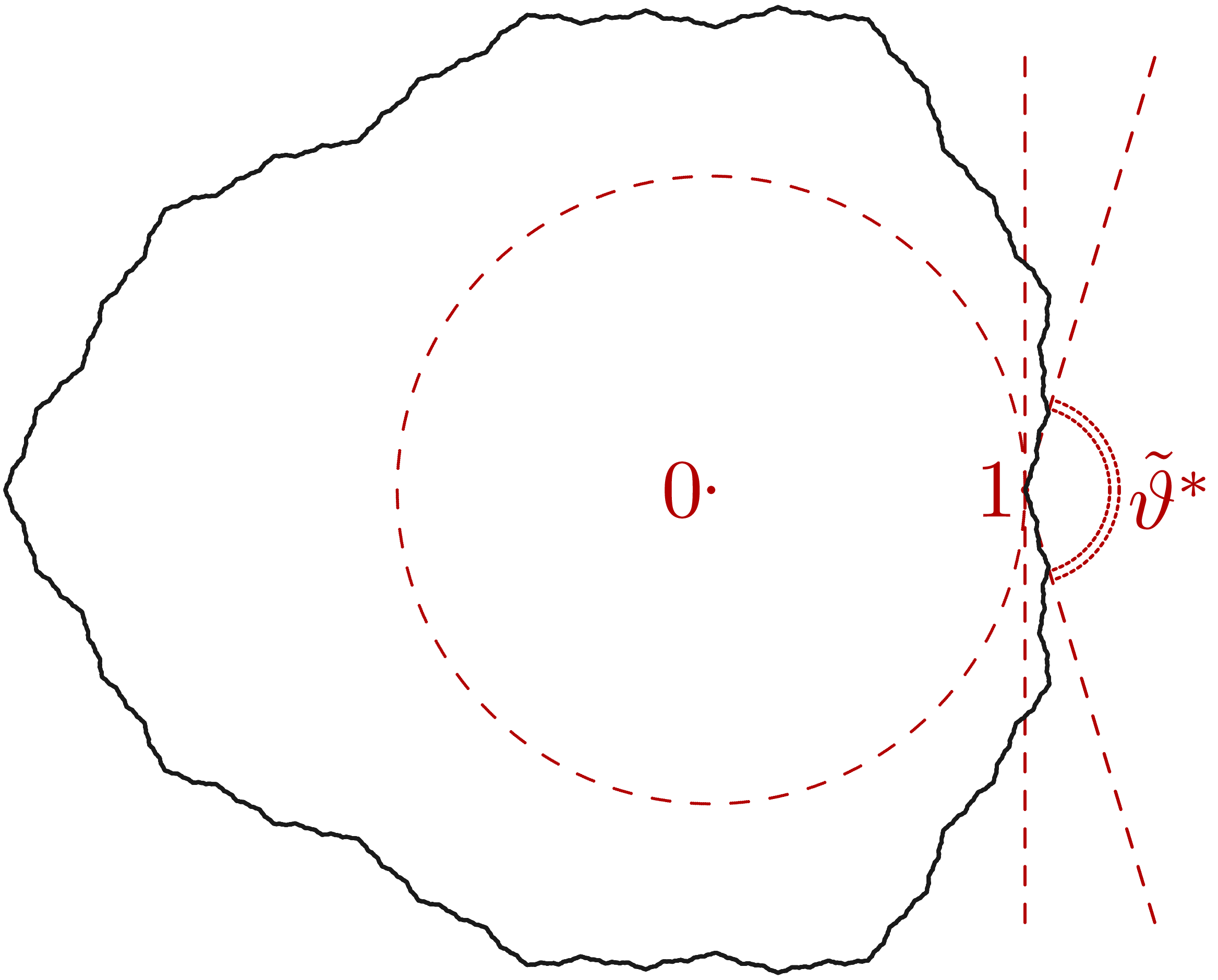
– this is the maximal angle of a sector of arbitrarily small radius in the neighborhood of 1 that lies entirely in the filled Julia set for the function P(z).Its complement
 $\tilde\vartheta^*=2\pi-\theta^*$
is illustrated in Figure 1, taken from [Reference Kutsenko12].
Julia set for the polynomial
 $P(z)=0.1z+0.5z^2+0.4z^3$
. It is the boundary of the open filled Julia set
 $\mathscr{J}_P$
(
 $\mathscr{J}_P=\mathscr{J}_P^{\kern1pt 0}$
for this case), which is the domain of definition for the analytic function
 $\Phi$
, see (7), since
 $P_t(z)\to0$
when
 $z\in \mathscr{J}_P^{\kern1pt 0}$
, and the convergence to zero is exponentially fast with the factor
 $p_1=P'(0)$
. The unit disk belongs to
 $\mathscr{J}_P^{\kern1pt 0}$
.

The Fourier coefficients of the one-periodic functions
 $$(K^{n+1}\cdot L)(z)=\sum_{m=-\infty}^{m=+\infty}\vartheta_{nm}{\mathrm{e}}^{2\pi\mathrm{i}mz}, \quad n\geqslant0,$$
are needed to formulate the main result, as well as the Taylor coefficients of the analytic function
 \begin{equation} A(z)=\frac{\Phi^{-1}(z)}{z\Psi(\Phi^{-1}(z))}=\sum_{n=0}^{+\infty}A_nz^n.\end{equation}
Theorem 1. If
 $\theta^*>\pi$
, then
 \begin{equation} p_\mathrm{imm}(x)=\sum_{n=0}^{+\infty}A_nx^{-\!\log_{\mu}\big(p_1^{n+1}q_0\big)-1}B_n(\!-\!\log_{\mu}x), \quad x>0, \end{equation}
where
 $\log_{\mu}\cdot=\ln\cdot/\ln\mu$
, and the one-periodic functions
 $B_n(z)$
are defined by
 \begin{equation} B_n(z) = \sum_{m=-\infty}^{m=+\infty}\frac{\vartheta_{nm}{\mathrm{e}}^{2\pi\mathrm{i}mz}} {\Gamma\big({-}\big({\ln\big(p_1^{n+1}q_0\big)+2\pi\mathrm{i}m}\big)/{\ln \mu}\big)}. \end{equation}
Here,
 $\Gamma$
is the Gamma function. Substituting (12) into (11), we get a double series that converges super-exponentially fast in n and exponentially fast in m:
 \begin{equation} \biggl|\frac{A_n\vartheta_{nm}} {\Gamma\big({-}\big({\ln\big(p_1^{n+1}q_0\big)+2\pi\mathrm{i}m}\big)/{\ln \mu}\big)}\biggr| \leqslant C{\mathrm{e}}^{-\alpha n\ln\!(n+1)-\beta|m|} \end{equation}
for some constants
 $\alpha,\beta,C>0$
.
Remark 1. Clearly, the critical angle satisfies
 $\theta^*\geqslant\pi$
, since the unit disk belongs to the filled Julia set for any probability-generating function P(z). We demand a little more:
 $\theta^*>\pi$
. While the assumption has a natural interpretation in terms of the geometry of the associated Julia set, its role in the present paper is purely auxiliary, namely to ensure the convergence of the double series. For concrete examples, the condition can be verified directly by constructing the associated Julia set. A more systematic study of this geometric condition, including extreme configurations and sharper estimates, will be presented elsewhere.
Usually, the Fourier coefficients of
 $B_n(z)$
are small, except for the zeroth one. The reason for the more precise estimates of the form (13) lies in the width of the strip in the complex plane on which the functions
 $B_n(z)$
are defined. The width is large enough. Hence, the Fourier coefficients of
 $B_n(z)$
decay quickly. This phenomenon is known in physics and biology in relation to other objects; see, e.g., [Reference Costin and Giacomin4, Reference Derrida, Itzykson and Luck5, Reference Derrida, Manrubia and Zanette6]. This fact allows us to define a good, quickly computed approximation of the density,
 \begin{equation} \tilde p_\mathrm{imm}(x) = \sum_{n=0}^N \frac{(K^{n+1}\cdot L)(0)A_n}{\Gamma\big({-}\!\log_{\mu}\big(p_1^{n+1}q_0\big)\big)}x^{-\!\log_{\mu}\big(p_1^{n+1}q_0\big)-1}, \quad x > 0,\end{equation}
with some moderate N. To evaluate K(0) and L(0), we can use fast-converging methods similar to those developed in, for example, [Reference Kutsenko12]. The computation of
 $A_n$
is generally explicit, because
 $\Phi^{-1}(z)$
satisfies the Poincaré-type functional equation
 \begin{equation} \Phi^{-1}(p_1z)=P(\Phi^{-1}(z)), \qquad \Phi^{-1}(z)\sim z, \quad z\to0,\end{equation}
and the composition
 $\Psi(\Phi^{-1}(z))$
satisfies
 \begin{equation} Q(\Phi^{-1}(z))\Psi(\Phi^{-1}(p_1z))=q_0\Psi(\Phi^{-1}(z)), \qquad \Psi(\Phi^{-1}(0))=1.\end{equation}
Substituting Taylor expansions in (15) and (16), we can find Taylor coefficients for both functions step by step. Then we can use them to find
 $A_n$
in (10).
The approximation (14) does not contain oscillatory terms. However, they may play some role. Let us define the following approximations:
 \begin{equation} \tilde p_{M,\mathrm{imm}}(x) = \sum_{n=0}^{N}A_nx^{-\!\log_{\mu}\big(p_1^{n+1}q_0\big)-1} \sum_{m=-M}^{m=M}\frac{\vartheta_{nm}{\mathrm{e}}^{-2\pi\mathrm{i}m\!\log_{\mu}x}} {\Gamma\big({-}\big({\ln\big(p_1^{n+1}q_0\big)+2\pi\mathrm{i}m}\big)/{\ln \mu}\big)}\end{equation}
with some moderate N. In other words, we replace
 $B_n$
in (11) and (12) by its initial segment of the Fourier series of length
 $2M+1$
.
As an illustration, we compare the density computed by (9) and (14) for the case
 \begin{equation} P(z)=p_1z+(1-p_1)z^2, \qquad Q(z)=q_0+(1-q_0)z.\end{equation}
To calculate (9), we take the interval
 $y \in [\!-\!2000, 2000]$
(or rather [0, 2000], utilizing symmetry) and divide it into
 $10^6$
points to apply the trapezoidal rule; the function
 $\Pi_\mathrm{imm}$
is computed up to 70 iterations of P. In (14), we take
 $N=10$
. For the calculations, Embarcadero Delphi Rad Studio Community Edition and the NesLib.Multiprecision library were used. This software provides a convenient environment for programming and well-functioning basic functions for high-precision computations. All algorithms related to the article’s subject, including efficient parallelization, were developed by the author (AK). The program is available in [Reference Kutsenko14]. We use 128-bit quadruple precision instead of the standard 64-bit double precision. The comparison results are quite good, at least for moderate values of x; see Figure 2. In particular, the areas under the plotted curves are
 $1\pm10^{-2}$
. Thus, the density values at which the curves may significantly differ are quite small. The approximation using (14) is calculated in real time, while the calculation using (9) takes several minutes on an Intel Core i7-7700HQ processor.

Nevertheless, the absence of oscillatory terms in (14) becomes visible for large x. In Figure 3(a), the approximations (14) and (17) are compared on the interval
 $x\in[3,8]$
. We take
 $N=30$
in both formulas, instead of
 $N=10$
, which was sufficient for
 $x\in[0,4]$
in Figure 2(a). Other parameters, such as the number of iterations, nodes, and the integration interval, remain the same. As expected,
 $\tilde p_\mathrm{imm}(x)$
and
 $\tilde p_{0,\mathrm{imm}}(x)$
are almost identical because the oscillatory terms are small enough. However, the spurious oscillations in
 $\tilde p_\mathrm{imm}(x)$
and
 $\tilde p_{0,\mathrm{imm}}(x)$
are reduced in the more accurate
 $\tilde p_{1,\mathrm{imm}}(x)$
and
 $\tilde p_{2,\mathrm{imm}}(x)$
due to the appearance in the sum (17) of natural oscillating terms that dampen false oscillations.


After performing proper normalization, we can also observe natural (non-spurious) density oscillations in the vicinity of
 $x=0$
, which arise due to logarithmically periodic terms
 $B_n$
in (11); see Figure 3(b). The analog of this phenomenon is illustrated in [Reference Kutsenko13] for the classical case without immigration. Note that on
 $x\in(0,0.1]$
the approximation (17) works well even for small
 $M=1$
and
 $N=3$
, while (9) did not for
 $x\to0$
. This happened even when we increased the number of iterations and nodes to
 $10^2$
and
 $2\cdot10^6$
, respectively, compared with the previous examples. The integration interval is also increased to
 $y\in[\!-\!3000,3000]$
.
2. Proof of Theorem 1
The analog of
 $\Phi(z)$
, see (7) and (1)–(3), is
 \begin{equation*} \Phi_\mathrm{imm}(z)=\lim_{t\to+\infty}(p_1q_0)^{-t}P_{\mathrm{imm},t}(z)=\Phi(z)\Psi(z),\end{equation*}
where
 \begin{equation} \Psi(z) = \lim_{t\to+\infty}q_0^{-t}Q(\underbrace{P\circ\cdots\circ P}_{t-1}(z))\cdots Q(P(z))\cdot Q(z) = \prod_{t=0}^{+\infty}q_0^{-1}Q(P_t(z)),\end{equation}
and
 $z\in\mathscr{J}_P^{\kern1pt 0}$
. The function
 $\Psi(z)$
is analytic inside the zero component of the filled Julia set
 $\mathscr{J}_P^{\kern1pt 0}$
related to the probability-generating function P(z). To show this, we note that Q(z) is defined in
 $\mathscr{J}_P^{\kern1pt 0}$
and
 $q_0^{-1}Q(P_t(z))-1\sim q_0^{-1}q_jP_t(z)^{\kern1pt j}$
for
 $t\to\infty$
and
 $z\in\mathscr{J}_P^{\kern1pt 0}$
. Here,
 $j>0$
is the minimal integer for which
 $q_j\ne0$
. Furthermore, using the fact that
 $P_t(z) \sim p_1^t \Phi(z)$
(see (7)) is exponentially small for large t and any fixed
 $z \in \mathscr{J}_P^{\kern1pt 0}$
, we can prove that the infinite product in (19) converges to an analytic function. This reasoning reiterates the arguments from, e.g., [Reference Milnor15] regarding the function
 $\Phi(z)$
. Definition (19) implies the functional equation
 \begin{equation} \Psi(z)=q_0^{-1}Q(z)\Psi(P(z)), \qquad \Psi(0)=1.\end{equation}
As we already discussed in the introduction, the full analog of
 $\Pi(z)$
, see (5) and (3), is
 \begin{equation} \Pi_\mathrm{imm}(z)=\lim_{t\to+\infty}P_{\mathrm{imm},t}(1-\mu^{-t}{z}),\end{equation}
and the density, see (4) for the classical case, is
 \begin{equation} p_\mathrm{imm}(x) = \frac1{2\pi}\int_{-\infty}^{+\infty}\Pi_\mathrm{imm}(\mathrm{i}y){\mathrm{e}}^{\mathrm{i}yx}\,{\mathrm{d}}y = \frac1{2\pi\mathrm{i}}\int_{\mathrm{i}{\mathbb R}}\Pi_\mathrm{imm}(z){\mathrm{e}}^{zx}\,{\mathrm{d}}z\end{equation}
in the case of immigration. Due to (5), (3), and (21), we have
 $\Pi_\mathrm{imm}(z)=\Pi(z)\cdot R(z)$
, where
 \begin{equation} R(z)=\prod_{t=1}^{+\infty}Q(\Pi(\mu^{-t}{z}))\end{equation}
satisfies the functional equation
 \begin{equation} R(\mu z)=R(z)Q(\Pi(z)), \qquad R(0)=1.\end{equation}
The infinite product (23) converges, because
 \begin{equation} Q(\Pi(\mu^{-t}{z}))-1\sim Q'(1)(\Pi(\mu^{-t}{z})-1)\sim Q'(1)\mu^{-t}{z}\end{equation}
for large t. The domain of definition of the analytic function R(z) contains at least a sector
 $\{z\colon |\mathop{\mathrm{arg}}\nolimits z|<\theta^*/2\}$
, since
 $\Pi(z)$
is analytic here by its definition (5) and the definition of
 $\mathscr{J}_P^{\kern1pt 0}$
. In other words, limiting P-compositions in (5) are well defined if
 $|\mathop{\mathrm{arg}}\nolimits z|<\theta^*/2$
because they lie inside
 $\mathscr{J}_P^{\kern1pt 0}$
, and we can apply the standard arguments from, e.g., [Reference Milnor15]. In particular,
 $\Pi(\{z\colon |\mathop{\mathrm{arg}}\nolimits z|<\theta^*/2\})\subset\mathscr{J}_P^{\kern1pt 0}$
, and if Q(z) is analytic in
 $\mathscr{J}_P^{\kern1pt 0}$
then R(z) is analytic in
 $\{z\colon |\mathop{\mathrm{arg}}\nolimits z|<\theta^*/2\}$
by (23) and (25).
Substituting
 $\Pi(z)$
instead of z into (20) and using (6), we obtain
 \begin{equation} Q(\Pi(z))\Psi(\Pi(\mu z))=q_0\Psi(\Pi(z)).\end{equation}
Eliminating
 $Q(\Pi(z))$
from (24) and (26), we deduce that
 ${R(\mu z)}{\Psi(\Pi(\mu z))}=q_0{R(z)}{\Psi(\Pi(z))}$
, which means that
 \begin{equation} L(z)\,:\!=\,q_0^{-z}{R(\mu^z)}{\Psi(\Pi(\mu^z))}\end{equation}
is a one-periodic function. Thus,
 \begin{equation*} R(z)=z^{\log_{\mu}q_0}\frac{L(\!\log_{\mu}z)}{\Psi(\Pi(z))},\end{equation*}
and
 \begin{equation} \Pi_\mathrm{imm}(z)=z^{\log_{\mu}q_0}\frac{\Pi(z)L(\!\log_{\mu}z)}{\Psi(\Pi(z))}.\end{equation}
For the classical case, the formula
 \begin{equation} \Pi(z)=\Phi^{-1}(z^{\log_{\mu}p_1}K(\!\log_{\mu}z))\end{equation}
follows from (8). Substituting (29) into (28) leads to
 \begin{equation} \Pi_\mathrm{imm}(z)=z^{\log_{\mu}(p_1q_0)}(K\cdot L)(\!\log_{\mu}z)A(z^{\log_{\mu}p_1}K(\!\log_{\mu}z)),\end{equation}
where
 \begin{equation} A(z)=\frac{\Phi^{-1}(z)}{z\Psi(\Phi^{-1}(z))}=\sum_{n=0}^{+\infty}A_nz^n\end{equation}
is a function analytic in some neighborhood of
 $z=0$
, with
 $A_0=1$
. In [Reference Kutsenko13], it is shown that the one-periodic and analytic function K(z) is defined at least in the strip
 \begin{equation} {\mathscr S}=\{|\mathop{\mathrm{Im}}\nolimits z|<{\theta^*}/({2\ln \mu})\}.\end{equation}
The same arguments apply to the one-periodic and analytic function L(z), see (27), which is also defined at least in the same strip as K(z), see (8). Indeed, the function
 $R(\mu^z)$
is defined for
 $z\in{\mathscr S}$
, since, as discussed above, R(z) is defined in the sector
 $\{z\colon |\mathop{\mathrm{arg}}\nolimits z|<\theta^*/2\}$
. The function
 $\Psi(z)$
, like
 $\Phi(z)$
, is defined in
 $\mathscr{J}_P^{\kern1pt 0}$
; see below (19). Therefore, we can apply the same arguments to
 $\Psi(\Pi(\mu^z))$
as to
 $\Phi(\Pi(\mu^z))$
in [Reference Kutsenko13]. Also, due to (30), we conclude that
 \begin{equation} \Pi_\mathrm{imm}(z)\to0, \quad z\to\infty, \quad |\mathop{\mathrm{arg}}\nolimits z|\leqslant\pi/2,\end{equation}
uniformly, due to the factor
 $z^{\log_{\mu}(p_1q_0)}$
with negative
 $\log_{\mu}(p_1q_0)$
. The boundedness of the function
 ${\mathrm{e}}^{zx}$
– given that
 $\mathop{\mathrm{Re}}\nolimits z$
is bounded and
 $x>0$
– together with (33) allows us to modify the integration contour in (22) based on Cauchy’s integral formula. We have
 \begin{equation} p_\mathrm{imm}(x) = \frac1{2\pi\mathrm{i}}\int_{\rho+\mathrm{i}{\mathbb R}}\Pi_\mathrm{imm}(z){\mathrm{e}}^{zx}\,{\mathrm{d}}z \quad \text{for all } \rho\geqslant0.\end{equation}
By (30) and (31), for any sufficiently large
 $\rho>0$
, we have
 \begin{equation} \Pi_\mathrm{imm}(z) = \sum_{n=0}^{+\infty}A_nz^{\log_{\mu}\big(p_1^{n+1}q_0\big)}(K^{n+1}\cdot L)(\!\log_{\mu}z), \quad \mathop{\mathrm{Re}}\nolimits z\geqslant\rho,\end{equation}
since
 $\log_{\mu}p_1<0$
and functions K and L are bounded on the strip
 ${\mathscr S}_1$
defined by
 \begin{equation} {\mathscr S}_1 = \{|\mathop{\mathrm{Im}}\nolimits z| \leqslant {\pi}/({2\ln \mu})\} \quad \big(\supset\{\log_{\mu} z\colon\mathop{\mathrm{Re}}\nolimits z\geqslant\rho\}\big).\end{equation}
Here, we use the fact that the strip
 ${\mathscr S}_1$
is smaller than the strip
 ${\mathscr S}$
, see (32), because
 $\theta^*>\pi$
. Therefore, the maximal moduli of the analytic and one-periodic functions K and L are finite in
 ${\mathscr S}_1$
.
According to Cauchy’s estimates, the Taylor coefficients
 $A_n$
exhibit at most exponential growth with respect to n. Namely,
 \begin{equation} |A_n|\leqslant C_2 r^n\end{equation}
for some
 $C_2>0$
and
 $r>0$
depending on the radius of convergence. Hence, the remainder
 \begin{equation*} \Pi_{\mathrm{imm},N}(z)=\sum_{n=N}^{+\infty}A_nz^{\log_{\mu}(p_1^{n+1}q_0)}(K^{n+1}\cdot L)(\!\log_{\mu}z)\end{equation*}
can be estimated as a geometric series,
 \begin{equation} |\Pi_{\mathrm{imm},N}(z)| \leqslant |z|^{\log_{\mu}{\kern-1pt}(p_1q_0)}\sum_{n=N}^{+\infty}C_3^n|z|^{n\!\log_{\mu}p_1} = \frac{|z|^{\log_{\mu}{\kern-1pt}(p_1q_0)}(C_3|z|^{\log_{\mu}p_1})^N}{1-C_3|z|^{\log_{\mu}p_1}}, \quad \mathop{\mathrm{Re}}\nolimits z\geqslant\rho,\end{equation}
for any sufficiently large
 $\rho>0$
, where the constant
 $C_3$
depends on the rate of growth of
 $A_n$
, see (37), and the maxima of the moduli of the functions K and L on the strip
 ${\mathscr S}_1$
, see (36). Due to (38) and
 $\log_{\mu}p_1<0$
, for any sufficiently large N and
 $\rho$
, the function
 ${\mathrm{e}}^{zx}\Pi_{{\rm imm},N}(z)$
is absolutely integrable on
 $\rho+\mathrm{i}{\mathbb R}$
, since
 ${\mathrm{e}}^{zx}$
is bounded on
 $\rho+\mathrm{i}{\mathbb R}$
for real x. Moreover, by (38), for any sufficiently large and fixed
 $\rho$
, the integral
 \begin{equation} \int_{\rho+\mathrm{i}{\mathbb R}}\Pi_{\mathrm{imm},N}(z){\mathrm{e}}^{zx}\,{\mathrm{d}}z\to0 \quad \mathrm{for}\ N\to+\infty.\end{equation}
We need the following lemma to show that the integrals of the first terms in (35) multiplied by
 ${\mathrm{e}}^{zx}$
exist.
Lemma 1. Let T(z) be an analytic one-periodic function defined on the strip
 ${\mathscr S}$
, see (32), with
 $\theta^*>\pi$
. Then, for any
 $x>0$
,
 $\rho>0$
, and
 $\alpha<0$
, the improper integral
 $\int_{\rho+\mathrm{i}{\mathbb R}}z^{\alpha}T(\!\log_{\mu}z){\mathrm{e}}^{zx}\,{\mathrm{d}}z$
exists.
Proof. To begin with, let us note that the integrand is well defined on the contour of integration. Indeed,
 $\log_{\mu}\{\rho+\mathrm{i}{\mathbb R}\}\subset{\mathscr S}$
, since
 $$ |\,{\mathrm{Im}} \ln(\rho+\mathrm{i}y)| = |\,{\mathrm{arg}} (\rho+\mathrm{i}y)|<\pi/2<\theta^*/2, \quad y\in{\mathbb R}. $$
Note also that the argument tends to
 $\pm\pi/2$
when
 $y\to\pm\infty$
. Integrating by parts, we have
 \begin{align*} \int_{\rho+\mathrm{i}C_1}^{\rho+\mathrm{i}C_2}z^{\alpha}T(\!\log_{\mu}z){\mathrm{e}}^{zx}\,{\mathrm{d}}z & = x^{-1}z^{\alpha}T(\!\log_{\mu}z){\mathrm{e}}^{zx}\big|_{\rho+\mathrm{i}C_1}^{\rho+\mathrm{i}C_2} \\ & \quad - x^{-1}\int_{\rho+\mathrm{i}C_1}^{\rho+\mathrm{i}C_2}z^{\alpha-1}(\alpha T(\!\log_{\mu}z) + (\ln \mu)^{-1}T'(\!\log_{\mu}z)){\mathrm{e}}^{zx}\,{\mathrm{d}}z, \end{align*}
which reduces the power of z by one. Moreover, the integrand in the right-hand side still satisfies the lemma conditions, and the two factors after
 $z^{\alpha-1}$
are bounded on
 $\rho+\mathrm{i}{\mathbb R}$
. Repeating this procedure, we can reduce the power of z so that the obtained integral converges absolutely when
 $C_{1}\to-\infty$
and
 $C_2\to+\infty$
. At the same time, according to the conditions of the lemma, e.g.
 $\alpha<0$
, the free terms tend to zero.
Taking into account Lemma 1 and the reasoning above (35)–(39), we can write
 \begin{align*} &\biggl|\frac1{2\pi\mathrm{i}}\int_{\rho-\mathrm{i}\infty}^{\rho+\mathrm{i}\infty}\Pi_\mathrm{imm}(z){\mathrm{e}}^{zx}\,{\mathrm{d}}z - \sum_{n=0}^{N-1}\frac{A_n}{2\pi\mathrm{i}}\int_{\rho-\mathrm{i}\infty}^{\rho+\mathrm{i}\infty}z^{\log_{\mu}(p_1^{n+1}q_0)}(K^{n+1}\cdot L)(\!\log_{\mu}z){\mathrm{e}}^{zx}\,{\mathrm{d}}z\biggr|\\&\qquad\quad = \biggl|\int_{\rho+\mathrm{i}{\mathbb R}}\Pi_{{\rm imm},N}(z){\mathrm{e}}^{zx}\,{\mathrm{d}}z\biggr|\to0 \quad \mathrm{for}\ N\to+\infty,\end{align*}
which means that
 \begin{equation} \frac1{2\pi\mathrm{i}}\int_{\rho-\mathrm{i}\infty}^{\rho+\mathrm{i}\infty}\Pi_\mathrm{imm}(z){\mathrm{e}}^{zx}\,{\mathrm{d}}z = \sum_{n=0}^{+\infty}\frac{A_n}{2\pi\mathrm{i}}\int_{\rho-\mathrm{i}\infty}^{\rho+\mathrm{i}\infty} z^{\log_{\mu}(p_1^{n+1}q_0)}(K^{n+1}\cdot L)(\!\log_{\mu}z){\mathrm{e}}^{zx}\,{\mathrm{d}}z\end{equation}
for
 $x>0$
and any sufficiently large
 $\rho>0$
. Due to (33),
 $\Pi_\mathrm{imm}(z)\to0$
for
 $z\to\infty$
with
 $\mathop{\mathrm{Re}}\nolimits z\geqslant0$
. Thus, (40) and (34) give
 \begin{equation} p_\mathrm{imm}(x) = \sum_{n=0}^{+\infty}\frac{A_n}{2\pi\mathrm{i}}\int_{\rho-\mathrm{i}\infty}^{\rho+\mathrm{i}\infty} z^{\log_{\mu}(p_1^{n+1}q_0)}(K^{n+1}\cdot L)(\!\log_{\mu}z){\mathrm{e}}^{zx}\,{\mathrm{d}}z, \quad x>0,\end{equation}
for all sufficiently large
 $\rho>0$
.
To continue, we need the following auxiliary statement. Suppose that
 $T(z)=\sum_{m\in{\mathbb Z}}\tau_m{\mathrm{e}}^{2\pi\mathrm{i}mz}$
is a one-periodic function analytic in the strip
 $| {\mathrm{Im}} z| < s$
for some
 $s>0$
. Then, for any sufficiently small
 $\delta>0$
, we have
 \begin{equation} |\tau_m| \leqslant {\mathrm{e}}^{-2\pi|m|(s-\delta)}\max_{x\in[0,1]}|T(x-\mathop{\mathrm{sign}}\nolimits\!(m)\mathrm{i}(s-\delta))|.\end{equation}
This statement follows easily from
 $\tau_m=\int_{[0,1]-\mathop{\mathrm{sign}}\nolimits\!(m)\mathrm{i}(s-\delta)}T(z){\mathrm{e}}^{-2\pi\mathrm{i}mz}\,{\mathrm{d}}z$
. Denote the Fourier coefficients of one-periodic functions
 $(K^{n+1}\cdot L)(z)$
by
 \begin{equation} (K^{n+1}\cdot L)(z)=\sum_{m=-\infty}^{m=+\infty}\vartheta_{nm}{\mathrm{e}}^{2\pi\mathrm{i}mz}, \quad n\geqslant0.\end{equation}
Remembering that K and L are analytic in the strip
 ${\mathscr S}$
, see (32), and applying (42) to (43), we obtain
 \begin{equation} |\vartheta_{nm}|\leqslant {\mathrm{e}}^{{-\pi |m|(\theta^*-\delta)}/{\ln \mu}} C_{\delta}^{n}\end{equation}
for any sufficiently small
 $\delta>0$
and some constants
 $C_{\delta}$
depending on the maximal values of K(z) and L(z) at the corresponding intervals within
 ${\mathscr S}$
. The Fourier coefficients
 $\vartheta_{nm}$
decay exponentially fast in m, so we can write
 \begin{align} & \frac{1}{2\pi\mathrm{i}}\int_{\rho-\mathrm{i}\infty}^{\rho+\mathrm{i}\infty} z^{\log_{\mu}(p_1^{n+1}q_0)}(K^{n+1}\cdot L)(\!\log_{\mu}z){\mathrm{e}}^{zx}\,{\mathrm{d}}z \nonumber \\& \qquad = \frac{1}{2\pi\mathrm{i}}\int_{\rho-\mathrm{i}\infty}^{\rho+\mathrm{i}\infty}\sum_{m=-\infty}^{m=+\infty} \vartheta_{nm}z^{({\ln(p_1^{n+1}q_0)+2\pi\mathrm{i}m})/{\ln \mu}}{\mathrm{e}}^{zx}\,{\mathrm{d}}z \nonumber \\ & \qquad = \sum_{m=-\infty}^{m=+\infty}\frac{1}{2\pi\mathrm{i}}\int_{\rho-\mathrm{i}\infty}^{\rho+\mathrm{i}\infty} \vartheta_{nm}z^{({\ln(p_1^{n+1}q_0)+2\pi\mathrm{i}m})/{\ln \mu}}{\mathrm{e}}^{zx}\,{\mathrm{d}}z \nonumber \\ & \qquad = \sum_{m=-\infty}^{m=+\infty} \frac{\vartheta_{nm}x^{-(({\ln(p_1^{n+1}q_0)+2\pi\mathrm{i}m})/{\ln \mu})-1}}{2\pi\mathrm{i}} \int_{\rho x-\mathrm{i}\infty}^{\rho x+\mathrm{i}\infty}z^{({\ln(p_1^{n+1}q_0)+2\pi\mathrm{i}m})/{\ln \mu}}{\mathrm{e}}^{z}\, {\mathrm{d}}z \nonumber \\ & \qquad = \sum_{m=-\infty}^{m=+\infty} \frac{\vartheta_{nm}x^{-(({\ln(p_1^{n+1}q_0)+2\pi\mathrm{i}m})/{\ln \mu})-1}} {\Gamma(\!-\!\big({\ln\big(p_1^{n+1}q_0\big)+2\pi\mathrm{i}m}\big)/{\ln \mu})} = x^{-({\ln(p_1^{n+1}q_0)}/{\ln \mu})-1}B_n(\!-\!\log_{\mu}x), \end{align}
where, for the last integral we used the Hankel representation of the
 $\Gamma$
function, see [Reference Whittaker and Watson17, Example 12.2.6, p. 254]. The one-periodic functions
 $B_n(z)$
are defined by
 \begin{equation} B_n(z) = \sum_{m=-\infty}^{m=+\infty}\frac{\vartheta_{nm}{\mathrm{e}}^{2\pi\mathrm{i}mz}} {\Gamma\big({-}\big({\ln\big(p_1^{n+1}q_0\big)+2\pi\mathrm{i}m}\big)/{\ln \mu}\big)}.\end{equation}
As we already discussed,
 $\vartheta_{nm}$
decays to zero exponentially fast in m. While the values of the Gamma function in (46) increase super-exponentially fast in n for fixed m, they are also exponentially small for large m and fixed n. More precisely, Stirling’s approximation of the Gamma function,
 \begin{equation*} \Gamma(z)=\sqrt{\frac{2\pi}z}\biggl(\frac{z}{{\mathrm{e}}}\biggr)^z\biggl(1+O\biggl(\frac1z\biggr)\biggr),\end{equation*}
gives
 \begin{equation} \biggl|\Gamma\biggl(-\frac{\ln\big(p_1^{n+1}q_0\big)+2\pi\mathrm{i}m}{\ln \mu}\biggr)\biggr| \geqslant \frac{\Upsilon}{\sqrt{\ln^2\big(p_1^{n+1}q_0\big)+4\pi^2m^2}}\end{equation}
for some constant
 $D>0$
and
 $$\Upsilon=D\exp\bigg\{{-}\frac{\ln\big(p_1^{n+1}q_0\big)}{\ln \mu}\ln\frac{\sqrt{\ln^2\big(p_1^{n+1}q_0\big)+4\pi^2m^2}}{\ln \mu} +\frac{\ln\big(p_1^{n+1}q_0\big)}{\ln \mu} - \frac{\pi^2|m|}{\ln \mu}\bigg\}.$$
The rate of growth in (47) is explicitly visible. Namely, choosing appropriate constants
 $D_0,\gamma_0>0$
and
 $\gamma_1\in{\mathbb R}$
, we can write
 \begin{equation} \biggl|\Gamma\biggl(-\frac{\ln\big(p_1^{n+1}q_0\big)+2\pi\mathrm{i}m}{\ln \mu}\biggr)\biggr| \geqslant D_0\frac{\exp\{\gamma_0(n+1)\ln\!(n+1)+\gamma_1n-{\pi^2|m|}/{\ln \mu}\}}{\sqrt{(n+1)^2+m^2}}.\end{equation}
Note that the square roots in the denominators, see (47) and (48), are equivalent up to multiplicative constants. Combining (48) with (44), eliminating
 $\sqrt{(n+1)^2+m^2}$
(which does not affect the leading exponential behavior, only the constants), and applying the condition
 $\theta^*-\delta>\pi$
for small
 $\delta>0$
, we derive
 \begin{equation} \biggl|\frac{\vartheta_{nm}} {\Gamma\big({-}\big({\ln\big(p_1^{n+1}q_0\big)+2\pi\mathrm{i}m}\big)/{\ln \mu}\big)}\biggr| \leqslant C_1{\mathrm{e}}^{-\alpha_1 n\ln\!(n+1)-\beta_1|m|}\end{equation}
for some constants
 $\alpha_1,\beta_1,C_1>0$
. Here, since
 $\gamma_0(n+1)\ln\!(n+1)$
grows asymptotically faster than the linear terms
 $\gamma_1n$
and
 $n\ln C_{\delta}$
, both the latter can be absorbed by the former for large n. The constant
 $C_1$
is then adjusted so that the inequality holds for small n as well. As we have already discussed, the Taylor coefficients of the analytic function A(z) do not grow faster than the exponential, see (37). Thus, if we multiply (49) by
 $A_n$
, the super-exponential decay by n does not change
 \begin{equation} \biggl|\frac{A_n\vartheta_{nm}} {\Gamma\big({-}\big({\ln\big(p_1^{n+1}q_0\big)+2\pi\mathrm{i}m}\big)/{\ln \mu}\big)}\biggr| \leqslant C_1C_2{\mathrm{e}}^{-\alpha_1 n\ln\!(n+1)+n\ln r-\beta_1|m|} \leqslant C{\mathrm{e}}^{-\alpha n\ln\!(n+1)-\beta|m|}\end{equation}
for some new constants
 $\alpha,C>0$
, and
 $\beta=\beta_1>0$
. The second inequality in (50) is valid for large
 $n>0$
because
 $\ln r\leqslant(\alpha_1-\alpha)\ln\!(n+1)$
for some
 $\alpha$
such that
 $0<\alpha<\alpha_1$
. Thus, the linear term of order n can be absorbed into the
 $n\ln\!(n+1)$
term, as already discussed below (49). The constant
 $C>0$
is chosen so that (50) is also valid for moderate and small n. Combining (41), (45), and (46), we also obtain
 \begin{equation*} p_\mathrm{imm}(x) = \sum_{n=0}^{+\infty}A_nx^{-({\ln\!(p_1^{n+1}q_0)}/{\ln \mu})-1}B_n(\!-\!\log_{\mu}x), \quad x>0.\end{equation*}
Acknowledgements
I would like to thank the anonymous reviewers for their valuable comments that improved the quality of the manuscript. AI tools were used to improve certain phrases in the text.
Funding information
This paper is a contribution to project S1 of the Collaborative Research Centre TRR 181 ‘Energy Transfer in Atmosphere and Ocean’ funded by the Deutsche Forschungsgemeinschaft (DFG, German Research Foundation) – Projektnummer 274762653.
Competing interests
There were no competing interests to declare which arose during the preparation or publication process of this article.
 P(z)=0.1z+0.5z2+0.4z3
 JP
 JP=JP0
 Φ
 Pt(z)→0
 z∈JP0
 p1=P′(0)
 JP0


 p1=0.3
 q0=0.5

 Open access

